Optimisation of 2D U-Net Model Components for Automatic Prostate Segmentation on MRI


Abstract
:1. Introduction
2. Background
2.1. Structure
2.2. The Convolution Layer
2.3. The Pooling Layer
2.4. Feature Maps
2.5. The Activation Layer
2.6. Dropout Layer
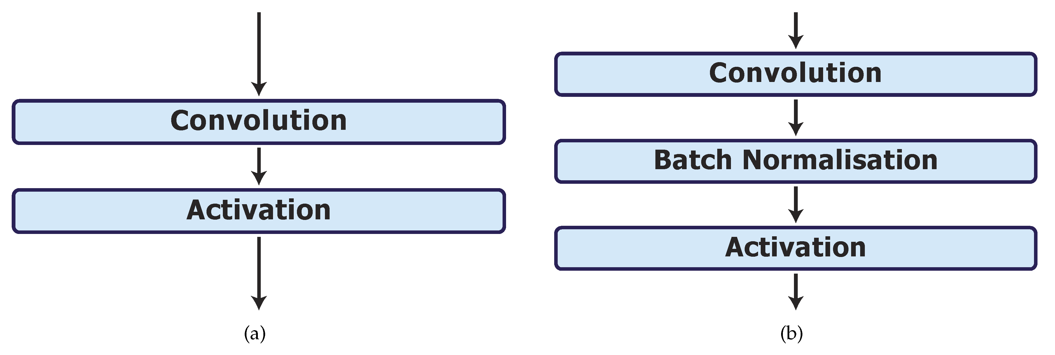
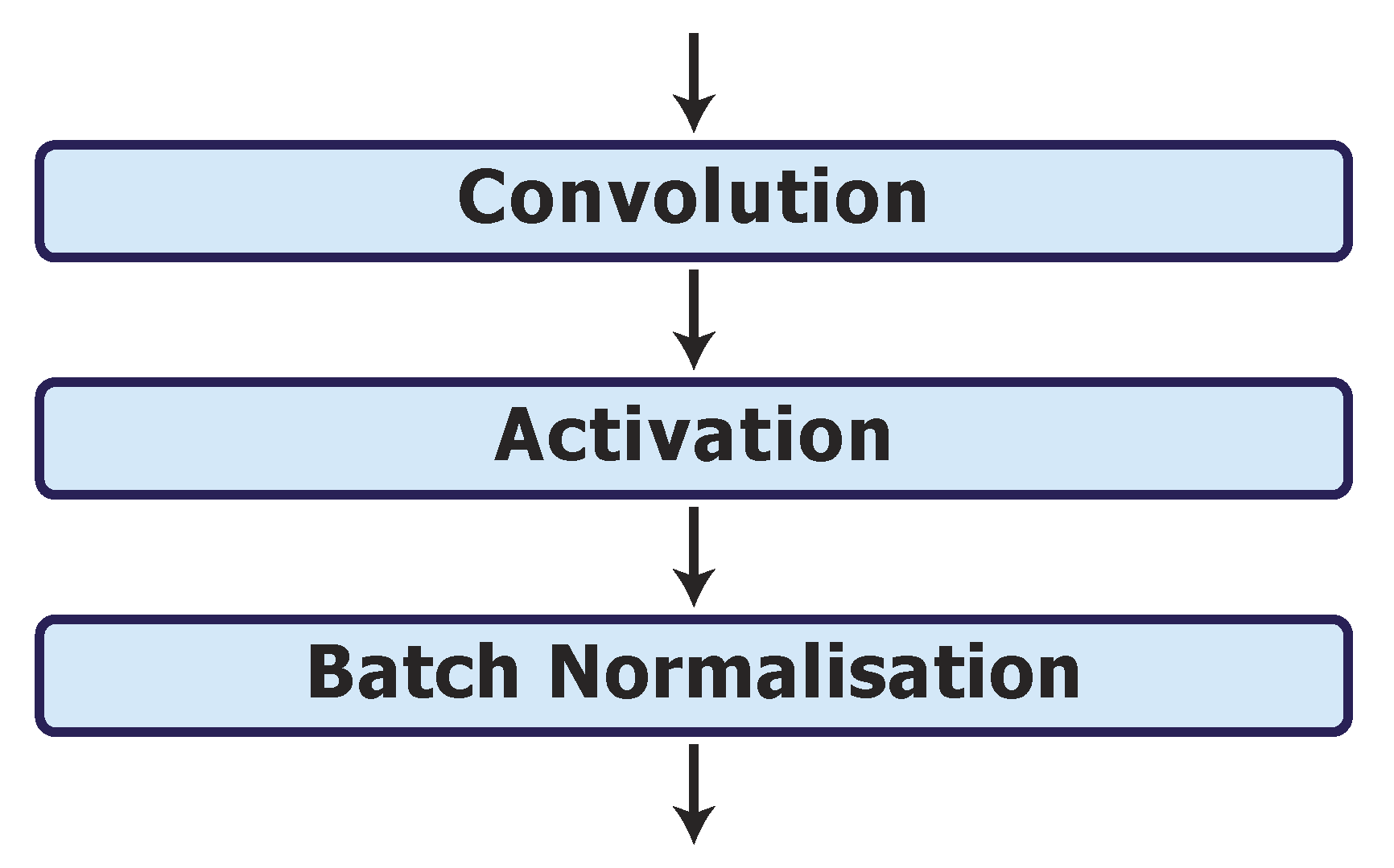
2.7. Batch Normalisation Layer
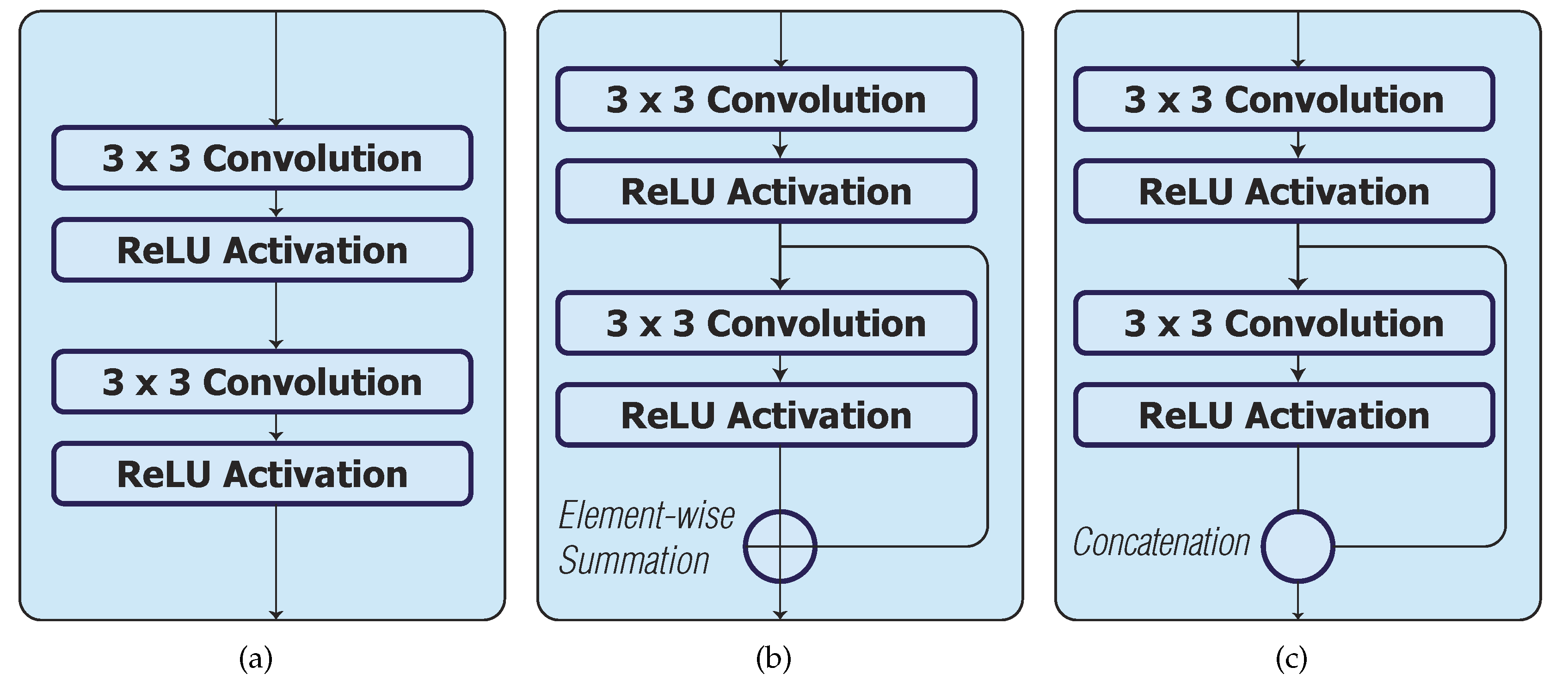
2.8. Skip Connections
3. Materials and Methods
3.1. Dataset
3.2. Performance Evaluation
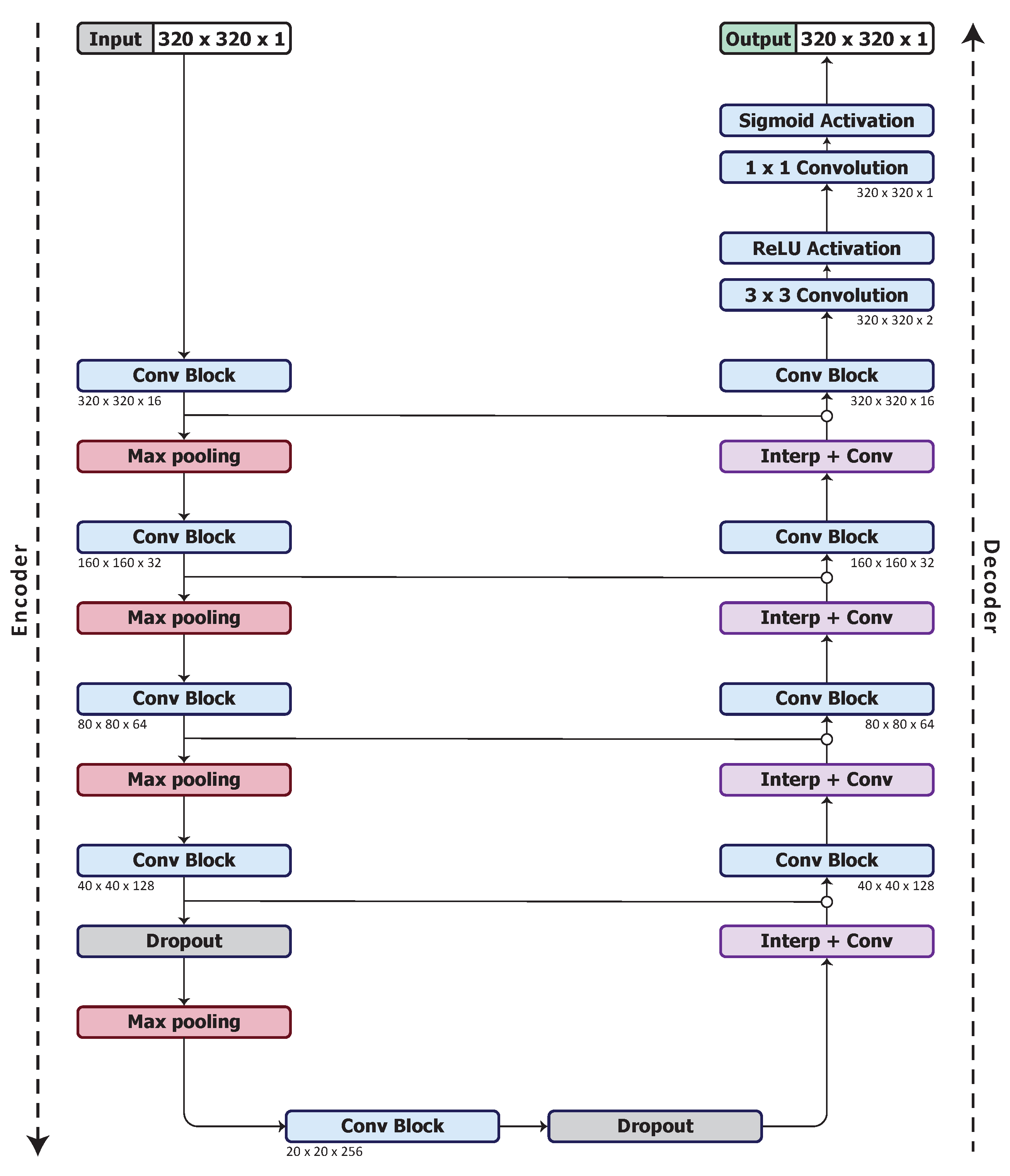
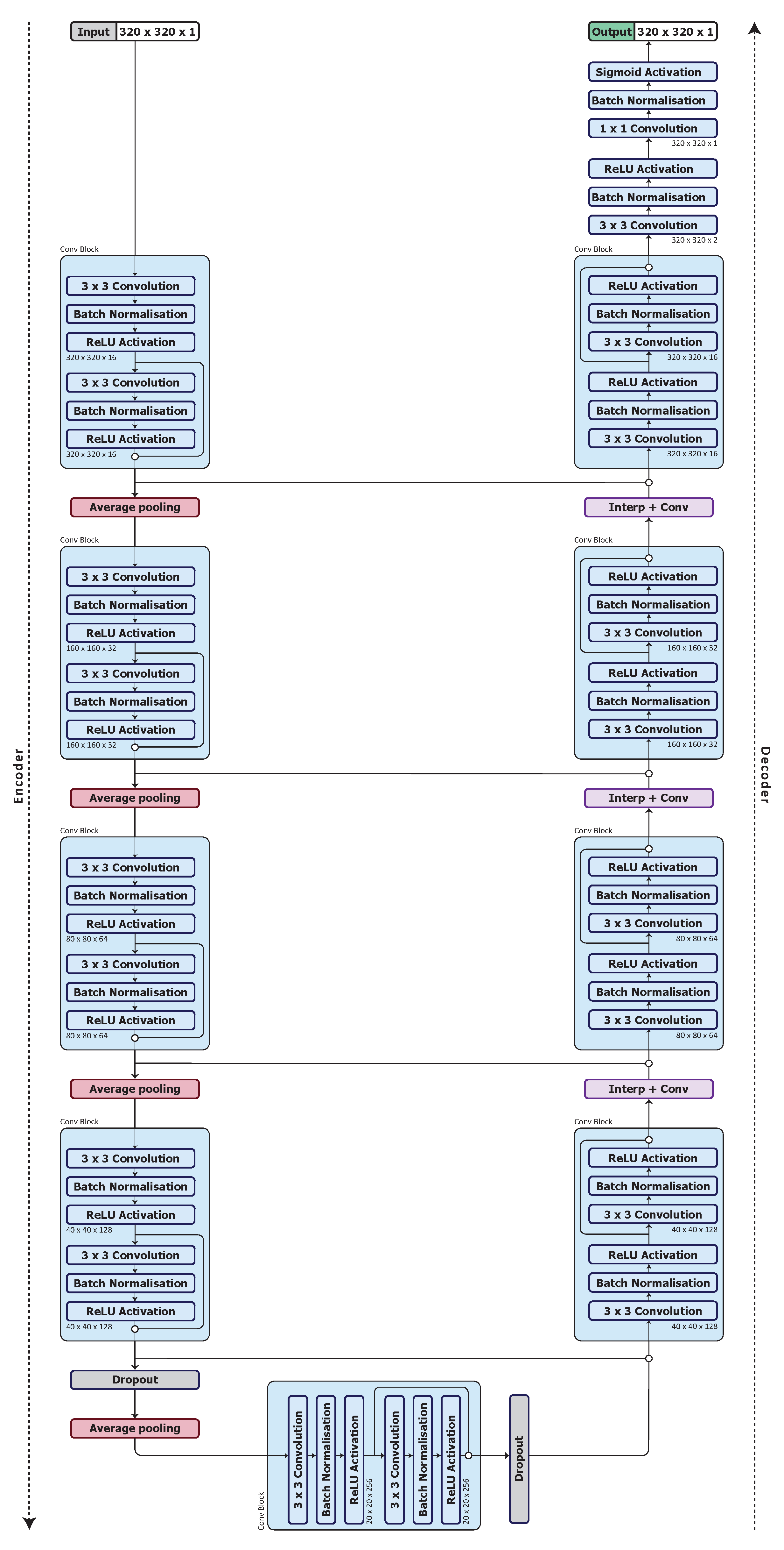
3.3. Model Architecture
3.4. Optimised Network Architecture
4. Results
4.1. Implementation on the Private Dataset
4.1.1. Training on the Private Dataset
4.1.2. Results on the Private Dataset
4.2. Implementation on the PROMISE12 Dataset
4.2.1. Training on the PROMISE12 dataset
4.2.2. Results on the PROMISE12 Test Set
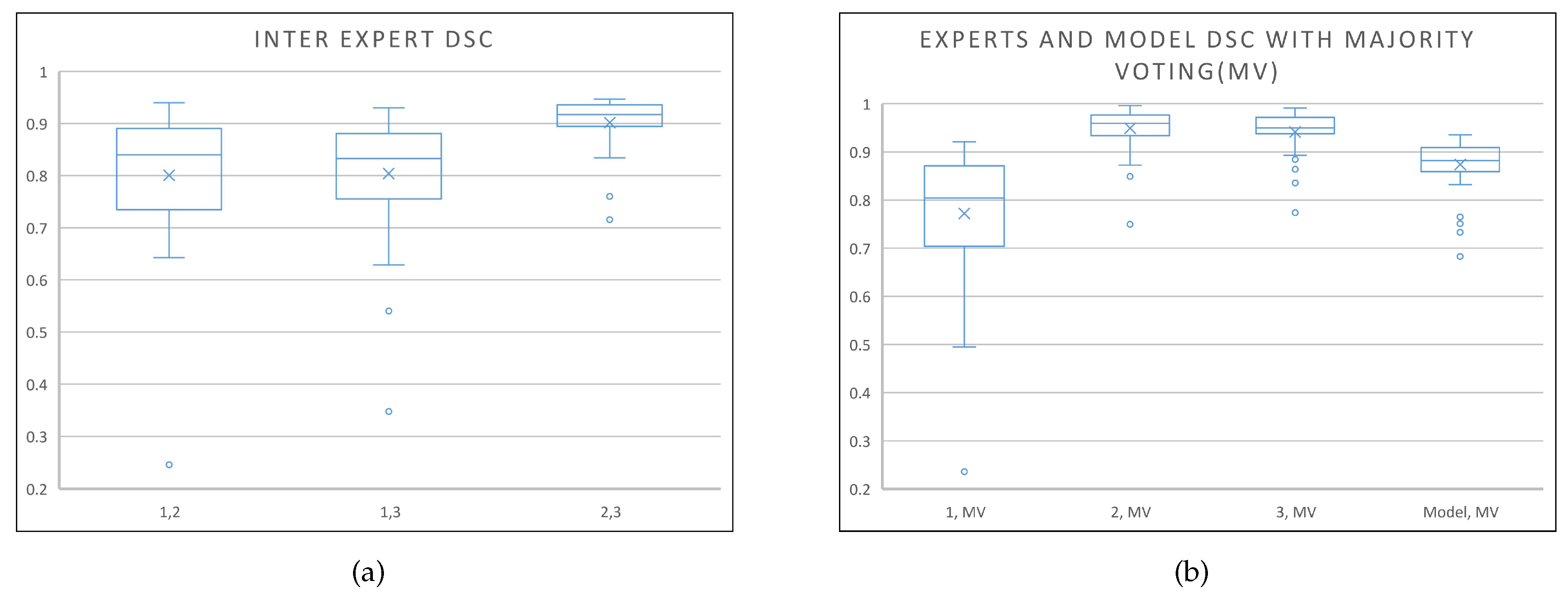
5. Discussion
6. Conclusions
Author Contributions
Funding
Acknowledgments
Conflicts of Interest
References
- Mishra, N.; Petrovic, S.; Sundar, S. A Knowledge-Light Nonlinear Case-Based Reasoning Approach to Radiotherapy Planning. In Proceedings of the 2009 21st IEEE International Conference on Tools with Artificial Intelligence, Newark, NJ, USA, 2–4 November 2009; pp. 776–783. [Google Scholar] [CrossRef]
- Dowling, J.A.; Fripp, J.; Chandra, S.; Pluim, J.P.W.; Lambert, J.; Parker, J.; Denham, J.; Greer, P.B.; Salvado, O. Fast Automatic Multi-atlas Segmentation of the Prostate from 3D MR Images. In Prostate Cancer Imaging. Image Analysis and Image-Guided Interventions; Madabhushi, A., Dowling, J., Huisman, H., Barratt, D., Eds.; Springer: Berlin/Heidelberg, Germany, 2011; pp. 10–21. [Google Scholar]
- Mahapatra, D. Semi-supervised learning and graph cuts for consensus based medical image segmentation. Pattern Recognit. 2017, 63, 700–709. [Google Scholar] [CrossRef]
- White, D.; Houston, A.S.; Sampson, W.F.D.; Wilkins, G.P. Intra- and Interoperator Variations in Region-of-Interest Drawing and Their Effect on the Measurement of Glomerular Filtration Rates. Clin. Nucl. Med. 1999, 24, 177–181. [Google Scholar] [CrossRef] [PubMed]
- Chandra, S.; Dowling, J.; Shen, K.; Pluim, J.; Greer, P.; Salvado, O.; Fripp, J. Automatic Segmentation of the Prostate in 3D Magnetic Resonance Images Using Case Specific Deformable Models. In Proceedings of the 2011 International Conference on Digital Image Computing: Techniques and Applications, Noosa, QLD, Australia, 6–8 December 2011; pp. 7–12. [Google Scholar] [CrossRef]
- Shahedi, M.; Ma, L.; Halicek, M.; Guo, R.; Zhang, G.; Schuster, D.M.; Nieh, P.; Master, V.; Fei, B. A semiautomatic algorithm for three-dimensional segmentation of the prostate on CT images using shape and local texture characteristics. In Medical Imaging 2018: Image-Guided Procedures, Robotic Interventions, and Modeling; Fei, B., Webster, R.J., III, Eds.; International Society for Optics and Photonics, SPIE: Bellingham, WA, USA, 2018; Volume 10576, pp. 280–287. [Google Scholar] [CrossRef]
- Chandra, S.S.; Dowling, J.A.; Shen, K.; Raniga, P.; Pluim, J.P.W.; Greer, P.B.; Salvado, O.; Fripp, J. Patient Specific Prostate Segmentation in 3-D Magnetic Resonance Images. IEEE Trans. Med. Imaging 2012, 31, 1955–1964. [Google Scholar] [CrossRef] [PubMed]
- Martin, S.; Troccaz, J.; Daanen, V. Automated segmentation of the prostate in 3D MR images using a probabilistic atlas and a spatially constrained deformable model. Med. Phys. 2010, 37, 1579–1590. [Google Scholar] [CrossRef] [PubMed] [Green Version]
- Wong, W.K.H.; Leung, L.H.T.; Kwong, D.L.W. Evaluation and optimization of the parameters used in multiple-atlas-based segmentation of prostate cancers in radiation therapy. Br. J. Radiol. 2016, 89, 20140732. [Google Scholar] [CrossRef] [PubMed] [Green Version]
- Gao, Y.; Shao, Y.; Lian, J.; Wang, A.Z.; Chen, R.C.; Shen, D. Accurate Segmentation of CT Male Pelvic Organs via Regression-Based Deformable Models and Multi-Task Random Forests. IEEE Trans. Med. Imaging 2016, 35, 1532–1543. [Google Scholar] [CrossRef] [Green Version]
- Cheng, R.; Turkbey, B.; Gandler, W.; Agarwal, H.K.; Shah, V.P.; Bokinsky, A.; McCreedy, E.; Wang, S.; Sankineni, S.; Bernardo, M.; et al. Atlas based AAM and SVM model for fully automatic MRI prostate segmentation. In Proceedings of the 2014 36th Annual International Conference of the IEEE Engineering in Medicine and Biology Society, Chicago, IL, USA, 26–30 August 2014; pp. 2881–2885. [Google Scholar] [CrossRef]
- Yang, M.; Li, X.; Turkbey, B.; Choyke, P.L.; Yan, P. Prostate Segmentation in MR Images Using Discriminant Boundary Features. IEEE Trans. Biomed. Eng. 2013, 60, 479–488. [Google Scholar] [CrossRef]
- Gao, Q.; Asthana, A.; Tong, T.; Hu, Y.; Rueckert, D.; Edwards, P. Hybrid Decision Forests for Prostate Segmentation in Multi-channel MR Images. In Proceedings of the 2014 22nd International Conference on Pattern Recognition, Stockholm, Sweden, 24–28 August 2014; pp. 3298–3303. [Google Scholar] [CrossRef]
- Kunjir, A.; Shaikh, B. A Survey on Machine Learning Algorithms for Building Smart Systems. Int. J. Innov. Res. Comput. Commun. Eng. 2017, 5, 1052–1058. [Google Scholar] [CrossRef]
- Fatima, M.; Pasha, M. Survey of Machine Learning Algorithms for Disease Diagnostic. J. Intell. Learn. Syst. Appl. 2017, 9, 1–16. [Google Scholar] [CrossRef] [Green Version]
- Yuan, Z.; Xu, C.; Sang, J.; Yan, S.; Hossain, M.S. Learning Feature Hierarchies: A Layer-Wise Tag-Embedded Approach. IEEE Trans. Multimed. 2015, 17, 816–827. [Google Scholar] [CrossRef]
- Bengio, Y. Learning Deep Architectures for AI; Essence of knowledge; Now Publishers: Delft The Netherlands, 2009; pp. 4–6. [Google Scholar]
- Shelhamer, E.; Long, J.; Darrell, T. Fully Convolutional Networks for Semantic Segmentation. IEEE Trans. Pattern Anal. Mach. Intell. 2017, 39, 640–651. [Google Scholar] [CrossRef] [PubMed]
- Ronneberger, O.; Fischer, P.; Brox, T. U-Net: Convolutional Networks for Biomedical Image Segmentation. In Medical Image Computing and Computer-Assisted Intervention—MICCAI 2015; Navab, N., Hornegger, J., Wells, W.M., Frangi, A.F., Eds.; Springer International Publishing: Cham, Switzerland, 2015; pp. 234–241. [Google Scholar]
- Huang, G.; Liu, Z.; Van Der Maaten, L.; Weinberger, K.Q. Densely Connected Convolutional Networks. In Proceedings of the 2017 IEEE Conference on Computer Vision and Pattern Recognition (CVPR), Honolulu, HI, USA, 21–26 July 2017; pp. 2261–2269. [Google Scholar] [CrossRef] [Green Version]
- Zhu, Q.; Du, B.; Turkbey, B.; Choyke, P.L.; Yan, P. Deeply-supervised CNN for prostate segmentation. In Proceedings of the 2017 International Joint Conference on Neural Networks (IJCNN), Anchorage, Alaska, AK, USA, 14–19 May 2017; pp. 178–184. [Google Scholar] [CrossRef] [Green Version]
- Xiangxiang, Q.; Yu, Z.; Bingbing, Z. Automated Segmentation Based on Residual U-Net Model for MR Prostate Images. In Proceedings of the 2018 11th International Congress on Image and Signal Processing, BioMedical Engineering and Informatics (CISP-BMEI), Beijing, China, 13–15 October 2018; pp. 1–6. [Google Scholar] [CrossRef]
- Zhu, Y.; Wei, R.; Gao, G.; Ding, L.; Zhang, X.; Wang, X.; Zhang, J. Fully automatic segmentation on prostate MR images based on cascaded fully convolution network. J. Magn. Reson. Imaging 2018, 49, 1149–1156. [Google Scholar] [CrossRef] [PubMed]
- Hassanzadeh, T.; Hamey, L.G.C.; Ho-Shon, K. Convolutional Neural Networks for Prostate Magnetic Resonance Image Segmentation. IEEE Access 2019, 7, 36748–36760. [Google Scholar] [CrossRef]
- Yuan, Y.; Qin, W.; Guo, X.; Buyyounouski, M.; Hancock, S.; Han, B.; Xing, L. Prostate Segmentation with Encoder-Decoder Densely Connected Convolutional Network (Ed-Densenet). In Proceedings of the 2019 IEEE 16th International Symposium on Biomedical Imaging (ISBI 2019), Venice, Italy, 8–11 April 2019; pp. 434–437. [Google Scholar] [CrossRef]
- Sahiner, B.; Pezeshk, A.; Hadjiiski, L.M.; Wang, X.; Drukker, K.; Cha, K.H.; Summers, R.M.; Giger, M.L. Deep learning in medical imaging and radiation therapy. Med. Phys. 2019, 46, e1–e36. [Google Scholar] [CrossRef] [Green Version]
- Zabihollahy, F.; Schieda, N.; Krishna Jeyaraj, S.; Ukwatta, E. Automated segmentation of prostate zonal anatomy on T2-weighted (T2W) and apparent diffusion coefficient (ADC) map MR images using U-Nets. Med. Phys. 2019, 46, 3078–3090. [Google Scholar] [CrossRef]
- Pattanayak, S. Pro Deep Learning with TensorFlow: A Mathematical Approach to Advanced Artificial Intelligence in Python; Apress: Berkeley, CA, USA, 2017; pp. 188–190. [Google Scholar] [CrossRef]
- Hou, L.; Samaras, D.; M Kurc, T.; Gao, Y.; E Davis, J.; Saltz, J. Patch-Based Convolutional Neural Network for Whole Slide Tissue Image Classification. In Proceedings of the 2016 IEEE Conf. Comput. Vis. Pattern Recognit. (CVPR), Vegas, NV, USA, 27–30 June 2016; Volume 2016, pp. 2424–2433. [Google Scholar] [CrossRef] [Green Version]
- Yan, K.; Li, C.; Wang, X.; Li, A.; Yuan, Y.; Feng, D.; Khadra, M.; Kim, J. Automatic prostate segmentation on MR images with deep network and graph model. In Proceedings of the 2016 38th Annual International Conference of the IEEE Engineering in Medicine and Biology Society (EMBC), Orlando, FL, USA, 16–20 August 2016; pp. 635–638. [Google Scholar] [CrossRef]
- He, B.; Xiao, D.; Hu, Q.; Jia, F. Automatic Magnetic Resonance Image Prostate Segmentation Based on Adaptive Feature Learning Probability Boosting Tree Initialization and CNN-ASM Refinement. IEEE Access 2018, 6, 2005–2015. [Google Scholar] [CrossRef]
- Haozhe, J.; Song, Y.; Huang, H.; Cai, W.; Xia, Y. HD-Net: Hybrid Discriminative Network for Prostate Segmentation in MR Images. In Proceedings of the 22nd International Conference on Medical Image Computing and Computer Assisted Intervention –MICCAI 2019, Shenzhen, China, 13–17 October 2019; pp. 110–118. [Google Scholar] [CrossRef]
- Milletari, F.; Navab, N.; Ahmadi, S.A. V-Net: Fully Convolutional Neural Networks for Volumetric Medical Image Segmentation. In Proceedings of the 2016 Fourth International Conference on 3D Vision (3DV), Stanford, CA, USA, 25–28 October 2016; pp. 565–571. [Google Scholar] [CrossRef] [Green Version]
- Kolařík, M.; Burget, R.; Uher, V.; Riha, K.; Dutta, M. Optimized High Resolution 3D Dense-U-Net Network for Brain and Spine Segmentation. Appl. Sci. 2019, 9, 404. [Google Scholar] [CrossRef] [Green Version]
- Dowling, J.A.; Sun, J.; Pichler, P.; Rivest-Hénault, D.; Ghose, S.; Richardson, H.; Wratten, C.; Martin, J.; Arm, J.; Best, L.; et al. Automatic Substitute Computed Tomography Generation and Contouring for Magnetic Resonance Imaging (MRI)-Alone External Beam Radiation Therapy From Standard MRI Sequences. Int. J. Radiat. Oncol. Biol. Phys. 2015, 93, 1144–1153. [Google Scholar] [CrossRef] [Green Version]
- Litjens, G.; Toth, R.; van de Ven, W.; Hoeks, C.; Kerkstra, S.; van Ginneken, B.; Vincent, G.; Guillard, G.; Birbeck, N.; Zhang, J.; et al. Evaluation of prostate segmentation algorithms for MRI: The PROMISE12 challenge. Med. Image Anal. 2014, 18, 359–373. [Google Scholar] [CrossRef] [Green Version]
- Chandra, S.S.; Dowling, J.A.; Greer, P.B.; Martin, J.; Wratten, C.; Pichler, P.; Fripp, J.; Crozier, S. Fast automated segmentation of multiple objects via spatially weighted shape learning. Phys. Med. Biol. 2016, 61, 8070–8084. [Google Scholar] [CrossRef] [Green Version]
- Lundervold, A.S.; Lundervold, A. An overview of deep learning in medical imaging focusing on MRI. Z. Für Med. Phys. 2019, 29, 102–127. [Google Scholar] [CrossRef] [PubMed]
- Li, X.; Chen, H.; Qi, X.; Dou, Q.; Fu, C.W.; Heng, P.A. H-DenseUNet: Hybrid Densely Connected UNet for Liver and Tumor Segmentation from CT Volumes. IEEE Trans. Med. Imaging 2018, 37, 2663–2674. [Google Scholar] [CrossRef] [PubMed] [Green Version]
- Peng, C.; Zhang, X.; Yu, G.; Luo, G.; Sun, J. Large Kernel Matters – Improve Semantic Segmentation by Global Convolutional Network. In Proceedings of the 2017 IEEE Conference on Computer Vision and Pattern Recognition (CVPR), Honolulu, HI, USA, 21–26 July 2017; pp. 1743–1751. [Google Scholar] [CrossRef] [Green Version]
- Long, J.; Shelhamer, E.; Darrell, T. Fully convolutional networks for semantic segmentation. In Proceedings of the 2015 IEEE Conference on Computer Vision and Pattern Recognition (CVPR), Boston, MA, USA, 7–12 June 2015; pp. 3431–3440. [Google Scholar] [CrossRef] [Green Version]
- Sugawara, Y.; Shiota, S.; Kiya, H. Checkerboard artifacts free convolutional neural networks. APSIPA Trans. Signal Inf. Process. 2019, 8, e9. [Google Scholar] [CrossRef] [Green Version]
- Odena, A.; Dumoulin, V.; Olah, C. Deconvolution and Checkerboard Artifacts. Distill 2016. [Google Scholar] [CrossRef]
- Springenberg, J.T.; Dosovitskiy, A.; Brox, T.; Riedmiller, M.A. Striving for Simplicity: The All Convolutional Net. arXiv 2014, arXiv:1412.6806. [Google Scholar]
- Bhat, S.S.; Hanumantharaju, M.C.; Gopalakrishna, M.T. An Exploration on Various Nonlinear Filters to Preserve the Edges of a Digital Image in Spatial Domain. In Proceedings of the 2015 International Conference on Advanced Research in Computer Science Engineering & Technology (ICARCSET 2015), ICARCSET ’15, Fukuoka, Japan, 27 July–1 August 2015; ACM: New York, NY, USA, 2015; pp. 51:1–51:7. [Google Scholar] [CrossRef]
- Burger, W.; Burge, M.J. Principles of Digital Image Processing: Fundamental Techniques, 1st ed.; Springer Publishing Company, Incorporated: Berlin/Heidelberg, Germany, 2009; pp. 116–130. [Google Scholar]
- LeCun, Y.; Haffner, P.; Bottou, L.; Bengio, Y. Object recognition with gradient-based learning. In Shape, Contour and Grouping in Computer Vision; Lecture Notes in Computer Science; Springer: Berlin, Germany, 1999; Volume 1681, pp. 319–345. [Google Scholar] [CrossRef]
- Lau, M.M.; Hann Lim, K. Review of Adaptive Activation Function in Deep Neural Network. In Proceedings of the 2018 IEEE-EMBS Conference on Biomedical Engineering and Sciences (IECBES), Sarawak, Malaysia, 3–6 December 2018; pp. 686–690. [Google Scholar] [CrossRef]
- Douglas, S.C.; Yu, J. Why RELU Units Sometimes Die: Analysis of Single-Unit Error Backpropagation in Neural Networks. In Proceedings of the 2018 52nd Asilomar Conference on Signals, Systems, and Computers, Pacific Grove, CA, USA, 28–31 October 2018; pp. 864–868. [Google Scholar] [CrossRef] [Green Version]
- Srivastava, N.; Hinton, G.; Krizhevsky, A.; Sutskever, I.; Salakhutdinov, R. Dropout: A Simple Way to Prevent Neural Networks from Overfitting. J. Mach. Learn. Res. 2014, 15, 1929–1958. [Google Scholar]
- Ioffe, S.; Szegedy, C. Batch Normalization: Accelerating Deep Network Training by Reducing Internal Covariate Shift. In Proceedings of the 32nd International Conference on Machine Learning, Lille, France, 6–11 July 2015; Bach, F., Blei, D., Eds.; PMLR: Lille, France, 2015; Volume 37, pp. 448–456. [Google Scholar]
- Gülçehre, Ç.; Bengio, Y. Knowledge Matters: Importance of Prior Information for Optimization. J. Mach. Learn. Res. 2016, 17, 1–32. [Google Scholar]
- He, K.; Zhang, X.; Ren, S.; Sun, J. Deep Residual Learning for Image Recognition. In Proceedings of the 2016 IEEE Conference on Computer Vision and Pattern Recognition (CVPR), Las Vegas, NV, USA, 27–30 June 2016; pp. 770–778. [Google Scholar] [CrossRef] [Green Version]
- Iglesias, J.E.; Sabuncu, M.R. Multi-atlas segmentation of biomedical images: A survey. Med. Image Anal. 2015, 24, 205–219. [Google Scholar] [CrossRef] [PubMed] [Green Version]
- Yeghiazaryan, V.; Voiculescu, I. An Overview of Current Evaluation Methods Used in Medical Image Segmentation; Technical Report RR-15-08; Department of Computer Science: Oxford, UK, 2015. [Google Scholar]
- Zhi, X. Unet. 2017. Available online: https://github.com/zhixuhao/unet (accessed on 3 July 2019).
- Kingma, D.P.; Ba, J. Adam: A Method for Stochastic Optimization. CoRR 2014. abs/1412.6980. [Google Scholar]
- Jain, A.; Fandango, A.; Kapoor, A. TensorFlow Machine Learning Projects: Build 13 Real-World Projects With Advanced Numerical Computations Using the Python Ecosystem; Packt Publishing: Birmingham, UK, 2018; pp. 59–60. [Google Scholar]
- Chollet, F. Keras. 2015. Available online: https://keras.io (accessed on 27 June 2019).
- Chen, W.; Zhang, Y.; He, J.; Qiao, Y.; Chen, Y.; Shi, H.; Tang, X. W-net: Bridged U-net for 2D Medical Image Segmentation. arXiv 2018, arXiv:1807.04459. [Google Scholar]
- Baldeon-Calisto, M.; Lai-Yuen, S.K. AdaResU-Net: Multiobjective adaptive convolutional neural network for medical image segmentation. Neurocomputing 2019. [Google Scholar] [CrossRef]
- Rundo, L.; Militello, C.; Russo, G.; Garufi, A.; Vitabile, S.; Gilardi, M.C.; Mauri, G. Automated Prostate Gland Segmentation Based on an Unsupervised Fuzzy C-Means Clustering Technique Using Multispectral T1w and T2w MR Imaging. Information 2017, 8, 49. [Google Scholar] [CrossRef] [Green Version]
- Lapa, P.; Castelli, M.; Gonçalves, I.; Sala, E.; Rundo, L. A Hybrid End-to-End Approach Integrating Conditional Random Fields into CNNs for Prostate Cancer Detection on MRI. Appl. Sci. 2020, 10, 338. [Google Scholar] [CrossRef] [Green Version]
- Schlemper, J.; Oktay, O.; Schaap, M.; Heinrich, M.; Kainz, B.; Glocker, B.; Rueckert, D. Attention gated networks: Learning to leverage salient regions in medical images. Med. Image Anal. 2019, 53, 197–207. [Google Scholar] [CrossRef] [PubMed]
- Hu, J.; Shen, L.; Albanie, S.; Sun, G.; Wu, E. Squeeze-and-Excitation Networks. IEEE Trans. Pattern Anal. Mach. Intell. 2019, 1. [Google Scholar] [CrossRef] [Green Version]
- Rundo, L.; Han, C.; Nagano, Y.; Zhang, J.; Hataya, R.; Militello, C.; Tangherloni, A.; Nobile, M.; Ferretti, C.; Besozzi, D.; et al. USE-Net: Incorporating squeeze-and-excitation blocks into U-net for prostate zonal segmentation of multi-institutional MRI datasets. Neurocomputing 2019, 365, 31–43. [Google Scholar] [CrossRef] [Green Version]


| Phase | Network | Components | |||||
|---|---|---|---|---|---|---|---|
| Downsampling | Upsampling | Skip Connection within Conv Block | Drop out | Batch Normalisation | Activation | ||
| 1 | UNet_S | Max Pooling | Interp+Conv | - | 0.5 | - | Relu |
| UNet_S1 | Max Pooling | Transposed Conv | - | 0.5 | - | Relu | |
| UNet_S2 | Strided Conv | Interp+Conv | - | 0.5 | - | Relu | |
| 2 | UNet_S.1 | Max Pooling | Interp+Conv | Summation | 0.5 | - | Relu |
| UNet_S1.1 | Max Pooling | Transposed Conv | Summation | 0.5 | - | Relu | |
| UNet_S2.1 | Strided Conv | Interp+Conv | Summation | 0.5 | - | Relu | |
| UNet_S.2 | Max Pooling | Interp+Conv | Concatenation | 0.5 | - | Relu | |
| UNet_S1.2 | Max Pooling | Transposed Conv | Concatenation | 0.5 | - | Relu | |
| UNet_S2.2 | Strided Conv | Interp+Conv | Concatenation | 0.5 | - | Relu | |
| 3 | UNet_S.2.1 | Max Pooling | Interp+Conv | Concatenation | 0 | - | Relu |
| 4 | UNet_S.2.0.1 | Max Pooling | Interp+Conv | Concatenation | 0.5 | Before Activation | Relu |
| 5 | UNet_S.2.0.1.1 | Avg Pooling | Interp+Conv | Concatenation | 0.5 | Before Activation | Relu |
| UNet_S.2.0.1.2 | RMS Pooling | Interp+Conv | Concatenation | 0.5 | Before Activation | Relu | |
| UNet_S.2.0.1.3 | L2 Pooling | Interp+Conv | Concatenation | 0.5 | Before Activation | Relu | |
| 6 | UNet_S.2.0.1.1.1 | Avg Pooling | Interp+Conv | Concatenation | 0.5 | Before Activation | LRelu |
| UNet_S.2.0.1.1.2 | Avg Pooling | Interp+Conv | Concatenation | 0.5 | After Activation | Relu | |
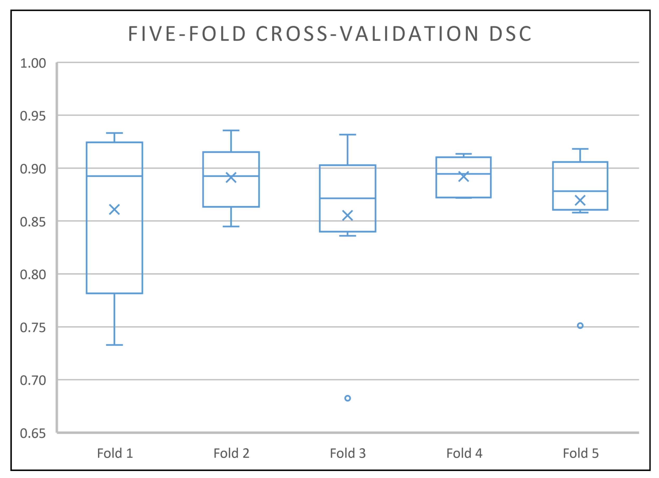
| Phase | Network | 5-Fold Cross-Validation DSC (%) | |||||
|---|---|---|---|---|---|---|---|
| Fold 1 | Fold 2 | Fold 3 | Fold 4 | Fold 5 | Avg | ||
| 1 | UNet_S | 85.28 | 86.86 | 83.36 | 86.16 | 81.53 | 84.64 |
| UNet_S1 | 85.26 | 83.04 | 79.66 | 81.43 | 79.16 | 81.70 | |
| UNet_S2 | 85.07 | 85.25 | 80.20 | 81.18 | 80.84 | 82.51 | |
| 2 | UNet_S.1 | 84.40 | 86.30 | 80.29 | 80.49 | 82.98 | 82.89 |
| UNet_S1.1 | 83.37 | 84.22 | 78.04 | 82.05 | 79.35 | 81.41 | |
| UNet_S2.1 | 83.70 | 82.53 | 79.19 | 82.68 | 82.03 | 82.03 | |
| UNet_S.2 | 85.46 | 88.01 | 82.91 | 84.76 | 84.89 | 85.21 | |
| UNet_S1.2 | 85.43 | 84.67 | 79.06 | 80.60 | 83.13 | 82.58 | |
| UNet_S2.2 | 85.28 | 81.63 | 81.08 | 84.35 | 80.33 | 82.53 | |
| 3 | UNet_S.2.1 | 82.31 | 84.97 | 80.11 | 84.08 | 81.47 | 82.59 |
| 4 | UNet_S.2.0.1 | 84.33 | 87.26 | 82.80 | 88.79 | 84.73 | 85.58 |
| 5 | UNet_S.2.0.1.1 | 84.02 | 88.87 | 83.97 | 89.23 | 85.07 | 86.23 |
| UNet_S.2.0.1.2 | 84.55 | 84.71 | 81.36 | 87.38 | 83.98 | 84.40 | |
| UNet_S.2.0.1.3 | 84.12 | 87.55 | 82.80 | 88.92 | 84.17 | 85.51 | |
| 6 | UNet_S.2.0.1.1.1 | 81.68 | 83.89 | 79.45 | 88.06 | 84.00 | 83.41 |
| UNet_S.2.0.1.1.2 | 84.64 | 87.95 | 82.68 | 87.75 | 84.68 | 85.54 | |
| Method | Mean DSC | Median DSC | Median ASD (mm) | Median Hausdorff (mm) |
|---|---|---|---|---|
| Multi-atlas | 0.80 | 0.82 | 2.04 | 13.3 |
| Weighted | 0.79 | 0.81 | 2.08 | 9.6 |
| Unweighted | - | 0.70 | 3.20 | 12.9 |
| UNet_S.2.0.1.1 | 0.87 | 0.88 | 0.72 | 4 |
| Rank | Team | Model | Model Type | Pre- | Post- | Mean DSC (%) | Overall Score |
|---|---|---|---|---|---|---|---|
| Processing | |||||||
| 35 | u3004443 | Z-Net | Single | Yes | Yes | 90.50 | 87.8068 |
| 59 | hkuandrewzhang (Revised_U-net) | Z-Net | Single | Yes | No | 90.24 | 87.3217 |
| 86 | wanlichen (WNet) | W-Net [60] | Stacked | No | No | 89.96 | 86.5028 |
| 92 | sho89512 | U-Net w/ Dense Dilated Block | Single | No | No | 88.98 | 86.3676 |
| 95 | fumin | RUCIMS (U-Net w/ Dense Dilated Block) | Single | Yes | No | 88.75 | 86.2589 |
| 122 | Indri92 (This paper) | UNet_S.2.0.1.1 (U-Net) | Single | No | No | 89.00 | 85.4954 |
| 140 | ddd52317102008 | Adversial Network | Adv. Net. | No | No | 87.90 | 84.5935 |
| 163 | mirzaevinom | MBIOS (U-Net) | Single | Yes | No | 88.06 | 83.6633 |
| 167 | ppppppppjw | U-Net w/ Dense Block | Single | No | No | 86.80 | 83.5027 |
| 168 | michaldrozdzal | UdeM 2D (ResNet) | Stacked | No | Yes | 87.42 | 83.4522 |
| 179 | mariabaldeon | AdaResU-Net [61] | Single | Yes | No | 86.51 | 82.7937 |
| 194 | wanlichen (WNet) | U-Net w/ skip connection | Single | No | No | 86.29 | 82.1644 |
© 2020 by the authors. Licensee MDPI, Basel, Switzerland. This article is an open access article distributed under the terms and conditions of the Creative Commons Attribution (CC BY) license (http://creativecommons.org/licenses/by/4.0/).
Share and Cite
Astono, I.P.; Welsh, J.S.; Chalup, S.; Greer, P. Optimisation of 2D U-Net Model Components for Automatic Prostate Segmentation on MRI. Appl. Sci. 2020, 10, 2601. https://doi.org/10.3390/app10072601
Astono IP, Welsh JS, Chalup S, Greer P. Optimisation of 2D U-Net Model Components for Automatic Prostate Segmentation on MRI. Applied Sciences. 2020; 10(7):2601. https://doi.org/10.3390/app10072601
Chicago/Turabian StyleAstono, Indriani P., James S. Welsh, Stephan Chalup, and Peter Greer. 2020. "Optimisation of 2D U-Net Model Components for Automatic Prostate Segmentation on MRI" Applied Sciences 10, no. 7: 2601. https://doi.org/10.3390/app10072601