On the Impact of the Rules on Autonomous Drive Learning

Abstract

Autonomous vehicles raise many ethical and moral issues that are not easy to deal with and that, if not addressed correctly, might be an obstacle to the advent of such a technological revolution. These issues are critical because autonomous vehicles will interact with human road users in new ways and current traffic rules might not be suitable for the resulting environment. We consider the problem of learning optimal behavior for autonomous vehicles using Reinforcement Learning in a simple road graph environment. In particular, we investigate the impact of traffic rules on the learned behaviors and consider a scenario where drivers are punished when they are not compliant with the rules, i.e., a scenario in which violation of traffic rules cannot be fully prevented. We performed an extensive experimental campaign, in a simulated environment, in which drivers were trained with and without rules, and assessed the learned behaviors in terms of efficiency and safety. The results show that drivers trained with rules enforcement are willing to reduce their efficiency in exchange for being compliant to the rules, thus leading to higher overall safety.

1. Introduction

In recent years, autonomous vehicles have attracted a lot of interest from both industrial and research groups [1,2]. The reasons for this growth are the technological advancement in the automotive field, the availability of faster computing units, and the increasing diffusion of the so-called Internet of Things. Autonomous vehicles collect a huge amount of data from the vehicle and from the outside environment, and are capable of processing these data in real-time to assist decision-making on the road. The amount of collected information and the need for real-time computing make the design of the driving algorithms a complex task to carry out with traditional techniques. Moreover, the sources of information may be noisy or may provide ambiguous information that could therefore negatively affect the outcome of the driving algorithm. The combination of these factors makes it very hard, if not unfeasible, to define the driver behavior by developing a set of hand-crafted rules. On the other side, the huge amount of data available can be leveraged by suitable machine learning techniques. The rise of deep learning in the last decade has proven its power in many fields, including self-driving cars development, and enabled the development of machines that take actions based on images collected by a front camera as the only source of information [3], or even using a biological inspired event-driven camera [4].

The use of simulations and synthetic data [5] for training have allowed to assess neural networks capabilities in many different realistic environments and different degrees of complexity. Many driving simulators have been designed, from the low-level ones that allow the drivers to control the hand brake of their car [6], to higher-level ones, in which the drivers can control their car acceleration and lane-change [7]. Some simulators model the traffic in an urban road network [8], some others model car’s intersection access [9,10,11,12], or roundabout insertion [13].

In a near future scenario, the first autonomous vehicles on the roads will have to make decisions in a mixed traffic environment. Autonomous vehicles will have to be able to cope with radically different road agents, i.e., agents powered by machines capable of processing information way more quickly than human drivers and human drivers that could occasionally take unexpected actions. There will hardly be a single authority to control each car in a centralized fashion and thus every autonomous vehicle will have to take decisions on its own, treating all the other road agents as part of the environment. It may very well be the case that current traffic rules do not fit a scenario with self-driving cars.

In this work, we investigate to which extent the traffic rules affect the drivers optimization process. The problem of finding the optimal driving behavior subjected to some traffic rules is highly relevant because it provides a way to define allowed behaviors for autonomous drivers, possibly without the need to manually craft those behaviors. A first approach for solving this problem consists of defining hard constraints on driver behavior and replacing forbidden actions with fallback ones [14]. Such an approach leads to drivers which are not explicitly aware of the rules. If those hard constraints were removed, driver behavior could change in unpredictable ways. Another approach consists in punishing behaviors that are not compliant with the rules, thus discouraging drivers from taking those behaviors again. In this work, we investigate this second approach based on punishing undesired behaviors. In this scenario, drivers have to learn the optimal behavior that balances a trade-off between being compliant with the rules and driving fast while avoiding collisions. A scenario in which drivers have the chance of breaking the rules is particularly relevant because it could address the complex ethics issues regarding self-driving cars in a more flexible way (those issues are fully orthogonal to our work, however).

We perform the optimization of the self-driving controllers using Reinforcement Learning (RL), which is a powerful framework used to find the optimal policy for a given task according to a trial-and-error paradigm. In this framework, we consider the possibility of enforcing traffic rules directly into the optimization process, as part of the reward function. Experimental results show that it is therefore possible to reduce unwanted behaviors with such approach.

2. Related Works

The rise of Reinforcement Learning (RL) [15] as an optimization framework for learning artificial agents, and the outstanding results of its combination with neural networks [16], have recently reached many new grounds, becoming a promising technique for the automation of driving tasks. Deep learning advances have proved that a neural network is highly effective in automatically extracting relevant features from raw data [17], as well as allowing an autonomous vehicle to take decisions based on information provided by a camera [3,4]. However, these approaches may not capture the complexity of planning decisions or predicting other drivers’ behavior, and their underlying supervised learning approach could be unable to cope with multiple complex sub-problems at once, including sub-problems not relevant to the driving task itself [18]. There are thus many reasons to consider a RL self-driving framework, which can tackle driving problems by interacting with an environment and learning from experience [18].

An example of an autonomous driving task implementation, based on Inverse Reinforcement Learning (IRL), was proposed by Sharifzadeh et al. [5]. The authors claimed that, in such a large state space task as driving, IRL can be effective in extracting the reward signal, using driving data from experts demonstrations. End-to-end low-level control through a RL driver was done by Jaritz et al. [6], in a simulated environment, based on the racing game TORCS, in which the driver has to learn full control of its car, that is steering, brake, gas, and even hand brake to enforce drifting. Autonomous driving is a challenging task for RL because it needs to ensure functional safety and every driver has to deal with the potentially unpredictable behavior of others [14]. One of the most interesting aspects of autonomous driving is learning how to efficiently cross an intersection, which requires providing suitable information on the intersection to the RL drivers [9], as well as correctly negotiating the access with other non-learning drivers and observing their trajectory [10,11]. Safely accessing to an intersection is a challenging task for RL drivers, due to the nature of the intersection itself, which may be occluded, and possible obstacles might not be clearly visible [12]. Another interesting aspect for RL drivers is learning to overtake other cars, which can be a particularly challenging task, depending on the shape of the road section in which the cars are placed [19], but also depending on the vehicles size, as in [20], where a RL driver learns to control a truck-trailer vehicle in an highway with other regular cars. The authors of [21,22] provided extensive classifications of the AI state-of-the-art techniques employed in autonomous driving, together with the degrees of automation that are possible for self-driving cars.

Despite the engineering advancements in designing self-driving cars, a lack of legal framework for these vehicles might slow down their coming [23]. There are also important ethical and social considerations. It has been proposed to address the corresponding issues as an engineering problem, by translating them into algorithms to be handled by the embedded software of a self-driving car [24]. This way the solution of a moral dilemma should be calculated based on a given set of rules or other mechanisms—although the exact practical details and, most importantly, their corresponding implications, are unclear. The problem of autonomous vehicles regulation is particularly relevant in mixed-traffic scenarios, as stated by Nyholm and Smids [25] and Kirkpatrick [26], as human drivers may behave in unpredictable ways to the machines. This problem could be mitigated by providing human drivers with more technological devices to help them drive more similar to robotic drivers, but mixed traffic ethics certainly introduce much deeper and more difficult problems [25].

A formalization of traffic rules for autonomous vehicles was provided by Rizaldi and Althoff [27], according to which a vehicle is not responsible for a collision if satisfying all the rules while colliding. Another driving automation approach based on mixed traffic rules is proposed in [28], where the rules are inspired by current traffic regulation. Traffic rules synthesis could even be automated, as proposed in [29], where a set of rules is evolved to ensure traffic efficiency and safety. The authors considered rules expressed by means of a language generated from a Backus–Naur Form grammar [30], but other ways to express spatiotemporal properties have been proposed [31,32]. Given the rules, the task of automatically finding the control strategy for robotics systems with safety rules is considered in [33], where the agents have to solve the task while minimizing the number of violated rules. AI safety can be inspired by humans, who intervene on agents in order to prevent unsafe situations, and then by training an algorithm to imitate the human intervention [34], thus reducing the amount of human labour required. A different strategy is followed by [35], where the authors defined a custom set of traffic rules based on the environment, the driver, and the road graph. With these rules, a RL driver learns to safely make lane-changing decisions, where the driver’s decision making is combined with the formal safety verification of the rules, to ensure that only safe actions are taken by the driver A similar approach is considered in [7], where the authors replaced the formal safety verification with a learnable safety belief module, as part of the driver’s policy.

3. Model

We consider a simple road traffic scenario in the form of a directed graph where the road sections are edges, and the intersections are vertices. Each road element is defined by continuous linear space in the direction of its length, and an integer number of lanes. In this scenario, a fixed number of cars move on the road graph according to their driver decisions for a given number of discrete time steps.

3.1. Road Graph

A road graph is a directed graph $G=(S,I)$ in which edges E represent road sections, and vertices I represent road intersections. Each road element $p\in G$ is connected to the next elements $n\left(p\right)\subset G$, with $n\left(p\right)\ne Ø$. Edges are straight one-way roads with one or more lanes. For each edge p, it holds that $n\left(p\right)\subset I$. Vertices can be either turns or crossroads, have exactly one lane, and are used to connect road sections. For each vertex p it holds that $n\left(p\right)\subset S$, and $\left|n\right(p\left)\right|=1$. Every road element $p\in G$ is defined by its length $l\left(p\right)\in {\mathbb{R}}^{+}$, and its number of lanes $w\left(p\right)\in \mathbb{N},w>0$. We do not take into account traffic lights or roundabouts in this scenario.

3.2. Cars

A car simulates a real vehicle that moves on the road graph G: its position can be determined at any time of the simulation in terms of the currently occupied road element and current lane. The car movement is determined in terms of two speeds—the linear speed along the road element and the lane-changing speed along the lanes of the same element. At each time step, the car state is defined by the tuple $(p,x,y,v_x,v_y,s)$, where $p\in \{S,I\}$ is the current road element, $x\in [0,l(p\left)\right]$ is the position on the road element, $y\in \{1,\cdots ,w(p\left)\right\}$ is the current lane, $v_x\in [0,v_{\max }]$ is the linear speed, $v_y\in \{-1,0,1\}$ is the lane-changing speed, and $s\in \{\mathrm{alive},\mathrm{dead}\}$ is the status (time reference is omitted for brevity). All the cars have the same length $l_{\mathrm{car}}$ and the same maximum speed $v_{\max }$.

At the beginning of a simulation, all cars are placed uniformly among the road sections, on all the lanes, ensuring that a minimum distance exists between cars $i,j$ on the same road element $p_i=p_j$, such that: $|x_i-x_j|>x_{\mathrm{gap}}$. The initial speeds for all the cars are $v_x=v_y=0$, and the status is $s=\mathrm{alive}$.

At the next time steps, if the status of a car is $s=\mathrm{dead}$, the position is not updated. Otherwise, if the status is $s=\mathrm{alive}$, the position of a car is updated as follows. Let $\left(a_x^{\left(t\right)},a_y^{\left(t\right)}\right)\in \{-1,0,1\}\times \{-1,0,1\}$ be the driver action composed, respectively, of $a_x^{\left(t\right)}$ accelerating action and $a_y^{\left(t\right)}$ lane-changing action (see details below). The linear speed and the lane-changing speed at time $t+1$ are updated accordingly with the driver action $\left(a_x^{\left(t\right)},a_y^{\left(t\right)}\right)$ at time t as:

$$\begin{array}{cc}\hfill v_x^{(t+1)}& =min\left(v_{\max },max\left(v_x^{\left(t\right)}+a_x^{\left(t\right)}{a}_{\max }\Delta t,0\right)\right)\hfill \end{array}$$

(1)

$$\begin{array}{cc}\hfill v_y^{(t+1)}& =a_y^{\left(t\right)}\hfill \end{array}$$

(2)

where $a_{\max }$ is the intensity of the instant acceleration and $\Delta t$ is the discrete time step duration. The car linear position on the road graph at time $t+1$ is updated as:

$$x^{(t+1)}=\left\{\begin{array}{cc}{x}^{\left(t\right)}+v_x^{(t+1)}\Delta t\hfill & \mathrm{if}{v}_x^{(t+1)}\Delta t\le x_{\mathrm{stop}}^{\left(t\right)}\hfill \\ v_x^{(t+1)}\Delta t-x_{\mathrm{stop}}^{\left(t\right)}\hfill & \mathrm{otherwise}\hfill \end{array}\right.$$

(3)

where $x_{\mathrm{stop}}$ is the distance ahead to the next road element, and is computed as:

$$x_{\mathrm{stop}}^{(t+1)}=l\left(p^{(t+1)}\right)-x^{(t+1)}$$

(4)

The car lane position at time $t+1$ is updated as:

$$y^{(t+1)}=min\left(w(p^{(t+1)}),max\left(y^{\left(t\right)}+v_y^{(t+1)},1\right)\right)$$

(5)

The road element at time $t+1$ is computed as:

$$p^{(t+1)}=\left\{\begin{array}{cc}{p}^{\left(t\right)}\hfill & \mathrm{if}{v}_x^{\left(t\right)}\Delta t\le x_{\mathrm{stop}}^{\left(t\right)}\hfill \\ \sim U\left(n\left(p^{\left(t\right)}\right)\right)\hfill & \mathrm{otherwise}\hfill \end{array}\right.$$

(6)

where U is the uniform distribution over the next road elements coming from p In other words, when exiting from an intersection, a car enters an intersection chosen randomly from $n\left(p^{\left(t\right)}\right)$.

Two cars collide, if the distance between them is smaller than the cars length $l_{\mathrm{car}}$. In particular, for any cars $(p,x,y,v_x,v_y,s)$, $(p^{\prime },x^{\prime },y^{\prime },v_x^{\prime },v_y^{\prime },s^{\prime })$, the status at time $t+1$ is updated as (we omit the time superscript for readability):

$$s=\left\{\begin{array}{cc}\mathrm{dead}\hfill & \mathrm{if}\left(p=p^{\prime }\wedge |x-x^{\prime }|<l_{\mathrm{car}}\right)\vee \left(p^{\prime }\in n\left(p\right)\wedge x_{\mathrm{stop}}+x^{\prime }<l_{\mathrm{car}}\right)\hfill \\ \mathrm{alive}\hfill & \mathrm{otherwise}\hfill \end{array}\right.$$

(7)

When a collision occurs, we simulate an impact by giving the leading car a positive acceleration of intensity $a_{\mathrm{coll}}$, while giving the following car a negative acceleration of intensity $-a_{\mathrm{coll}}$, for the next $t_{\mathrm{coll}}$ time steps. Collided cars are kept in the simulation for the next $t_{\mathrm{dead}}>t_{\mathrm{coll}}$ time steps of the simulation, thus acting as obstacles for the alive ones.

3.3. Drivers

A driver is an algorithm that is associated to a car. Each driver is able to sense part of its car variables and information from the road environment, and takes driving actions that affect its car state. Every driver ability to see obstacles on the road graph is limited to the distance of view $d_{\mathrm{view}}$.

3.3.1. Observation

For the driver of a car $(p,x,y,v_x,v_y,s)$, the set of visible cars in the jth relative lane, with $j\in \{-1,0,1\}$, is the union of the set $V_{\mathrm{same},j}$ of cars that are in the same segment and the same or adjacent lane and the set $V_{\mathrm{next}}$ of cars that are in one of the next segments $p^{\prime }\in n\left(p\right)$, in both cases with a distance shorter than $d_{\mathrm{view}}$:

$$\begin{array}{cc}\hfill V_{\mathrm{same},j}& =\left\{(p^{\prime },x^{\prime },y^{\prime },v_x^{\prime },v_y^{\prime },s^{\prime }):p^{\prime }=p\wedge 0<x^{\prime }-x\le d_{\mathrm{view}}\wedge y^{\prime }=y+j\right\}\hfill \end{array}$$

(8)

$$\begin{array}{cc}\hfill V_{\mathrm{next}}& =\left\{(p^{\prime },x^{\prime },y^{\prime },v_x^{\prime },v_y^{\prime },s^{\prime }):p^{\prime }\in n\left(p\right)\wedge x_{\mathrm{stop}}+x^{\prime }\le d_{\mathrm{view}}\right\}\hfill \end{array}$$

(9)

We remark that the set of cars $V_j=V_{\mathrm{same},j}\cup V_{\mathrm{next}}$ includes also the cars in the next segments: the current car is hence able to perceive cars in a intersection, when in a segment, or in the connected sections, when in an intersection, provided that they are closer than $d_{\mathrm{view}}$.

The driver’s observation is based on the concept of jth lane closest car $c_j^{\mathrm{closest}}$, based on the set $V_j$ defined above. For each driver, $c_j^{\mathrm{closest}}$ is the closest one in $V_j$:

$$c_j^{\mathrm{closest}}=\left\{\begin{array}{cc}\underset{(p^{\prime },x^{\prime },y^{\prime },v_x^{\prime },v_y^{\prime },s^{\prime })\in V_j}{arg\; min}\mathbb{1}(p^{\prime }=p)(x^{\prime }-x)+\mathbb{1}(p^{\prime }\ne p)(x_{\mathrm{stop}}+x^{\prime })\hfill & \mathrm{if}{V}_j\ne Ø\hfill \\ Ø\hfill & \mathrm{otherwise}\hfill \end{array}\right.$$

(10)

where $V_j=V_{\mathrm{same},j}\cup V_{\mathrm{next}}$ and $\mathbb{1}:\{\mathrm{false},\mathrm{true}\}\to \{0,1\}$ is the indicator function. Figure 1 illustrates two different examples of jth lane closest car, with $j=0$. We can see that the $c_j^{\mathrm{closest}}$ might not exist for some j, either if there is no car closer than $d_{\mathrm{view}}$ or if there is no such jth lane.

We define the closeness variables ${\delta }_{x,j}\in [0,d_{\mathrm{view}}]$, with $j\in \{-1,0,1\}$, as the distances to the jth lane closest cars $c_j^{\mathrm{closest}}$, if any, or $d_{\mathrm{view}}$, otherwise. Similarly, we define the relative speed variables ${\delta }_{v,j}\in [-v_{\max },v_{\max }]$, with $j\in \{-1,0,1\}$, as the speed difference of the current car with respect to the jth lane closest cars $c_j^{\mathrm{closest}}$, if any, or $v_{\max }$, otherwise.

At each time step of the simulation, each driver observes the distance from its car to the next road element, indicated by $x_{\mathrm{stop}}$, the current lane y, the current linear speed $v_x$, the status of its vehicle s, the road element type $e=\mathbb{1}(p\in S)$ its car is currently on, the closeness variables ${\delta }_{x,j}$, and the relative speed variable ${\delta }_{v,j}$. We define each driver observation as: $o=\left(x_{\mathrm{stop}},y,v_x,s,e,{\delta }_{x,-1},{\delta }_{x,0},{\delta }_{x,1},{\delta }_{v,-1},{\delta }_{v,0},{\delta }_{v,1}\right)$, therefore $o\in O=[0,l_{\max }]\times \{1,w_{\max }\}\times [0,v_{\max }]\times \{\mathrm{alive},\mathrm{dead}\}\times \{0,1\}\times {[0,d_{\mathrm{view}}]}^3\times {[-v_{\max },v_{\max }]}^3$.

3.3.2. Action

Each agent action is $a=\left(a_x,x_y\right)\in A=\{-1,0,1\}\times \{-1,0,1\}$. Intuitively $a_x$ is responsible for updating the linear speed in the following way: $a_x=1$ corresponds to accelerating, $a_x=-1$ corresponds to breaking, and $a_x=0$ keeps the linear speed unchanged. On the other hand $a_y$ is responsible for updating the lane-position in the following way: $a_y=1$ corresponds to moving to the left lane, $a_y=-1$ corresponds to moving to the right lane, and $a_y=0$ to keeping the lane-position unchanged.

3.4. Rules

A traffic rule is a tuple $(b,w)$ where $b:O\to \{false,true\}$ is the rule predicate, defined on the drivers observation space O, and $w\in \mathbb{R}$ is the rule weighting factor. The ith driver breaks a rule at a given time step t if the statement b that defines the rule is $b\left(o_i^{\left(t\right)}\right)=1$. We define a set of three rules $((b_1,w_1),(b_2,w_2),(b_3,w_3))$, described in the next sections, that we use to simulate the real-world traffic rules for the drivers. All the drivers are subjected to the rules.

3.4.1. Intersection Rule

In this road scenario, we do not enforce any junction access negotiation protocol, nor we consider traffic lights, and cars access interactions as in Figure 2. That is, there is no explicit reason for drivers to slow down when approaching a junction, other than the chances of collisions with other cars crossing the intersection at the same time. Motivated by this lack of safety at intersections, we define a traffic rule that punishes drivers approaching or crossing an intersection at high linear speed.

In particular, the driver in road element p such that $p\in I$ is an intersection, or equivalently $p\in S$ and its car is in the proximity of an intersection, denoted by $x_{\mathrm{stop}}<2l_{\mathrm{car}}$, breaks the intersection rule indicated by $(b_1,w_1)$ if traveling at linear speed $v_x>10$:

$$b_1\left(o\right)=\left\{\begin{array}{cc}1\hfill & \mathrm{if}\left(p\in I\vee x_{\mathrm{stop}}<2l_{\mathrm{car}}\right)\wedge v_x>10\hfill \\ 0\hfill & \mathrm{otherwise}\hfill \end{array}\right.$$

(11)

3.4.2. Distance Rule

Collisions may occur when traveling with insufficient distance from the car ahead, since it is difficult to predict the leading car behavior in advance. For this reason, we introduce a rule that punishes drivers that travel too close to the car ahead.

In particular, the driver observing $c_0^{\mathrm{closest}}$ closest car on the same lane breaks the distance rule indicated by $(b_2,w_2)$ if traveling at linear speed $v_x$ such that the distance traveled before arresting the vehicle is greater than ${\delta }_{x,0}-l_{\mathrm{car}}$, or, in other words:

$$b_2\left(o\right)=\left\{\begin{array}{cc}1\hfill & \mathrm{if}{\delta }_{x,0}-l_{\mathrm{car}}<2a_{\max }{v}_x^2\hfill \\ 0\hfill & \mathrm{otherwise}\hfill \end{array}\right.$$

(12)

3.4.3. Right Lane Rule

In this scenario, cars might occupy any lane on a road segment, without any specific constraint. This freedom might cause the drivers to unpredictably change lanes while traveling, thus endangering other drivers, who might not have the chance to avoid the oncoming collision. Motivated by this potentially dangerous behaviors, we define a rule that allows drivers to overtake when close to the car ahead, but punishes the ones leaving the right-most free lane on a road section.

In particular, the driver occupying road section $p\in S$, on non-rightmost lane $y>1$, breaks the right lane rule indicated by $(b_3,w_3)$ if the closest car on the right lane $c_{-1}^{\mathrm{closest}}$ is traveling at a distance ${\delta }_{x,-1}=d_{\mathrm{view}}$:

$$b_3\left(o\right)=\left\{\begin{array}{cc}1\hfill & \mathrm{if}p\in S\wedge y>1\wedge {\delta }_{x,-1}=d_{\mathrm{view}}\hfill \\ 0\hfill & \mathrm{otherwise}\hfill \end{array}\right.$$

(13)

3.5. Reward

Drivers are rewarded according to their linear speed, thus promoting efficiency. All cars involved in a collision, denoted by state $s=\mathrm{dead}$, are then arrested after the impact, thus resulting in zero reward for the next $t_{\mathrm{dead}}-t_{\mathrm{coll}}$ time steps, which implicitly promotes safety. Each driver reward at time t is:

$$r^{\left(t\right)}=\frac{v_x^{\left(t\right)}}{v_{\max }}-\sum _{i=1}^3{w}_i{b}_i\left(o^{\left(t\right)}\right)$$

(14)

where w are the weights of the rules.

3.6. Policy Learning

Each driver’s goal is to maximize the return over a simulation, indicated by ${\sum }_{t=0}^T{\gamma }^t{r}^{(t+1)}$, where $\gamma \in [0,1]$ is the discount factor and $T>0$ is the number of time steps of the simulation. The driver policy is the function ${\pi }_{\theta }:O\to A$ that maps observations to actions. We parameterize the drivers’ policy in the form of a feed-forward neural network, where $\theta$ is the set of parameters of the neural network. Learning the optimal policy corresponds to the problem of finding the values of $\theta$ that maximize the return over an entire simulation. We perform policy learning by means of RL.

4. Experiments

Our goal was to experimentally assess the impact of the traffic rules on the optimized policies, in terms of overall efficiency and safety. To this aim, we defined 3 tuples, which are, respectively, the reward tuple R, the efficiency tuple E, and the collision tuple C.

The reward tuple $R\in {\mathbb{R}}^{n_{\mathrm{car}}}$ is the tuple of individual rewards collected by the drivers during an episode, from $t=0$ to $t=T$, and is defined as:

$$R=\left(\sum _{t=0}^T{r}_1^{\left(t\right)},\cdots ,\sum _{t=0}^T{r}_{n_{\mathrm{cars}}}^{\left(t\right)}\right)$$

(15)

The efficiency tuple $E\in {\mathbb{R}}^{n_{\mathrm{car}}}$ is the tuple of sums of individual instant linear speed $v_x$ for each driver during an episode, from $t=0$ to $t=T$, and is defined as:

$$E=\left(\sum _{t=0}^T{v}_{x_1}^{\left(t\right)},\cdots ,\sum _{t=0}^T{v}_{x_{n_{\mathrm{cars}}}}^{\left(t\right)}\right)$$

(16)

The collision tuple $C\in {\mathbb{N}}^{n_{\mathrm{car}}}$ is the tuple of individual collisions for each driver during an episode, from $t=0$ to $t=T$, and is defined as:

$$C=\left(\sum _{t=0}^T\mathbb{1}\{s_1^{(t-1)}=\mathrm{alive}\wedge s_1^{\left(t\right)}=\mathrm{dead}\},\cdots ,\sum _{t=0}^T\mathbb{1}\{s_{n_{cars}}^{(t-1)}=\mathrm{alive}\wedge s_{n_{cars}}^{\left(t\right)}=\mathrm{dead}\}\right)$$

(17)

Each ith element $c_i$ of this tuple is defined as the number of times in which the ith driver change its car status $s_i$ from $s_i=\mathrm{alive}$ to $s_i=\mathrm{dead}$ between 2 consecutive time steps $t-1$ and t.

We considered 2 different driving scenarios in which we aimed at finding optimal policy parameters:y “no-rules”, in which traffic rules weighting factors are $w_1=w_1=w_3=0$, such that drivers are not punished for breaking the rules, and “rules”, in which traffic rules weighting factors are $w_1=w_2=w_3=1$, such that drivers are punished for breaking the rules, and all the rules have the same relevance.

Moreover, we considered 2 different collision scenarios:

(a)

cars are kept with status $s=\mathrm{dead}$ in the road graph for $t_{\mathrm{dead}}$ time steps, and then are removed; and

(b)

cars are kept with status $s=\mathrm{dead}$ in the road graph for $t_{\mathrm{dead}}$ time steps, and then their status is changed back into $s=\mathrm{alive}$.

The rationale for considering the second option is that the condition in which we remove collided cars after $t_{\mathrm{dead}}$ time steps may not be good enough for finding the optimal policy. This assumption could ease the task of driving for the non-collided cars, when the number of collided cars grows, and, on the other side, it might provide too few collisions to learn from.

We simulated $n_{\mathrm{cars}}$ cars sharing the same driver policy parameters and moving in the simple road graph in Figure 3 for T time steps. This road graph has 1 main intersection at the center, and 4 three-way intersections. All road segments $p\in S$ have the same length $l\left(p\right)$ and same number of lanes $w\left(p\right)$. We used the model parameters shown in

Table 1. Model and simulation parameters.

Param	Meaning	Value
$l_{\mathrm{car}}$	Car length	7
$t_{\mathrm{coll}}$	Impact duration	10
$t_{\mathrm{dead}}$	Collision duration	20
$d_{\mathrm{view}}$	Driver’s view distance	50
$v_{\max }$	Driver’s maximum speed	50
$a_{\max }$	Driver’s acceleration (deceleration)	2
$\Delta t$	Time step duration	0.2
$\left|S\right|$	Number of road sections	12
$\left|I\right|$	Number of road intersections	9
$w\left(p\right),p\in G$	Number of lanes	$\in \{1,2\}$
$l\left(p\right),p\in S$	Section length	100
$n_{\mathrm{car}}$	Cars in the simulation	40
T	Simulation time steps	500

and performed the simulations using Flow [36], a microscopic discrete-time continuous-space road traffic simulator that allows implementing our scenarios.

We repeated $n_{\mathrm{trials}}$ experiments in which we performed $n_{\mathrm{train}}$ training iterations in order to optimize the initial random policy parameters ${\theta }_{\mathrm{no}-\mathrm{rules}}$ and ${\theta }_{\mathrm{rules}}$. We collected the values, across the $n_{\mathrm{trials}}$ repetitions, of R, E, and C during the training.

We employed Proximal Policy Optimization (PPO) [37] as the RL policy optimization algorithm: PPO is a state-of-the-art actor-critic algorithm that is highly effective, while being almost parameters-free. We used the PPO default configuration (https://ray.readthedocs.io/en/latest/rllib-algorithms.html) with the parameters shown in

Table 2. Policy learning algorithm parameters.

Param	Meaning	Value
$n_{\mathrm{trial}}$	Number of trials	20
$n_{\mathrm{train}}$	Training iterations	500
$n_{\mathrm{car}}$	Cars in the simulation	40
$\gamma$	Discount factor	0.999

. The drivers policy is in the form of an actor-critic neural networks model, where each of the 2 neural networks is made of 2 hidden layers, each one with 256 neurons and hyperbolic tangent as activation function. The hidden layer parameters are shared between the actor and the critic networks: this is a common practice introduced by Mnih et al. [38] that helps to improve the overall performances of the model. The parameters of the actor network as well as the ones of the critic network are initially distributed according to the Xavier initializer [39].

5. Results

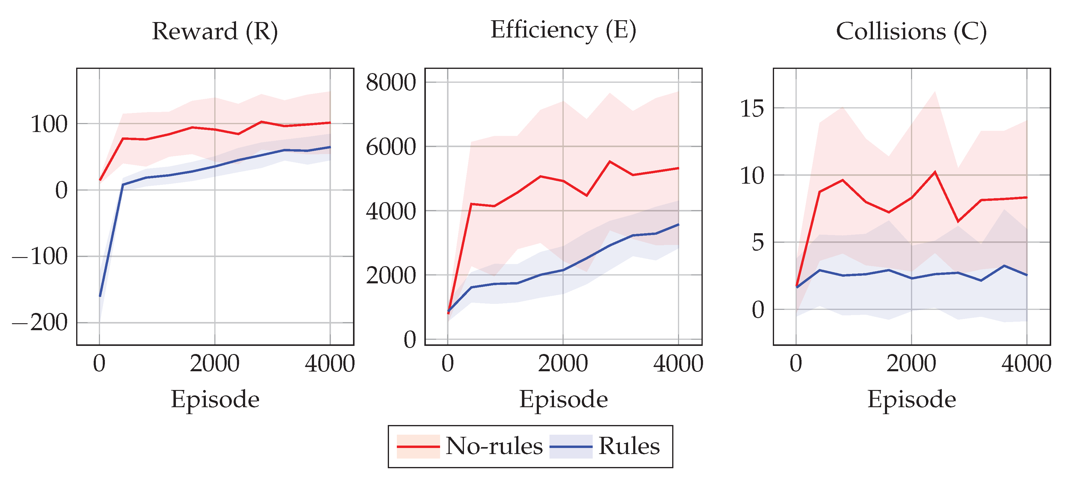
Figure 4 and Figure 5 show the training results in terms of the tuples R, E, and C for the 2 policies ${\theta }_{\mathrm{no}-\mathrm{rules}}$ and ${\theta }_{\mathrm{rules}}$ in the two collision scenarios considered.

In all experimental scenarios, the policy learned with rules shows driving behaviors that are less efficient than the ones achieved by the one without rules. On the other hand, the policy learned without rules is not even as efficient as it could theoretically be, due to the high number of collisions that make it difficult to avoid collided cars. Moreover, the values of E for the drivers employing the rules are distributed closer to the mean efficiency value, and thus we can assume this is due to the fact that the rules limit the space of possible behaviors to a smaller space with respect to the case without rules. In other words, rules seems to favor equity among drivers.

On the other hand, the policy learned with rules shows driving behaviors that are safer than the ones achieved by the one without rules. This may be due to the fact that training every single driver to avoid collisions based only on the efficiency reward is a difficult learning task, as well as because agents are not capable of predicting the other agents’ trajectories. On the other hand, we can see that the simple traffic rules that we have designed are effective at improving the overall safety.

In other words, these results show that, as expected, policies learned with rules are safer but less efficient than the ones without rules. Interestingly, the rules act also as a proxy for equality, as shown in Figure 4 and Figure 5, in particular for the efficiency values of E, where the blue shaded area is much thinner than the red one, meaning that all the $n_{\mathrm{car}}$ vehicles have similar efficiency.

Robustness to Traffic Level

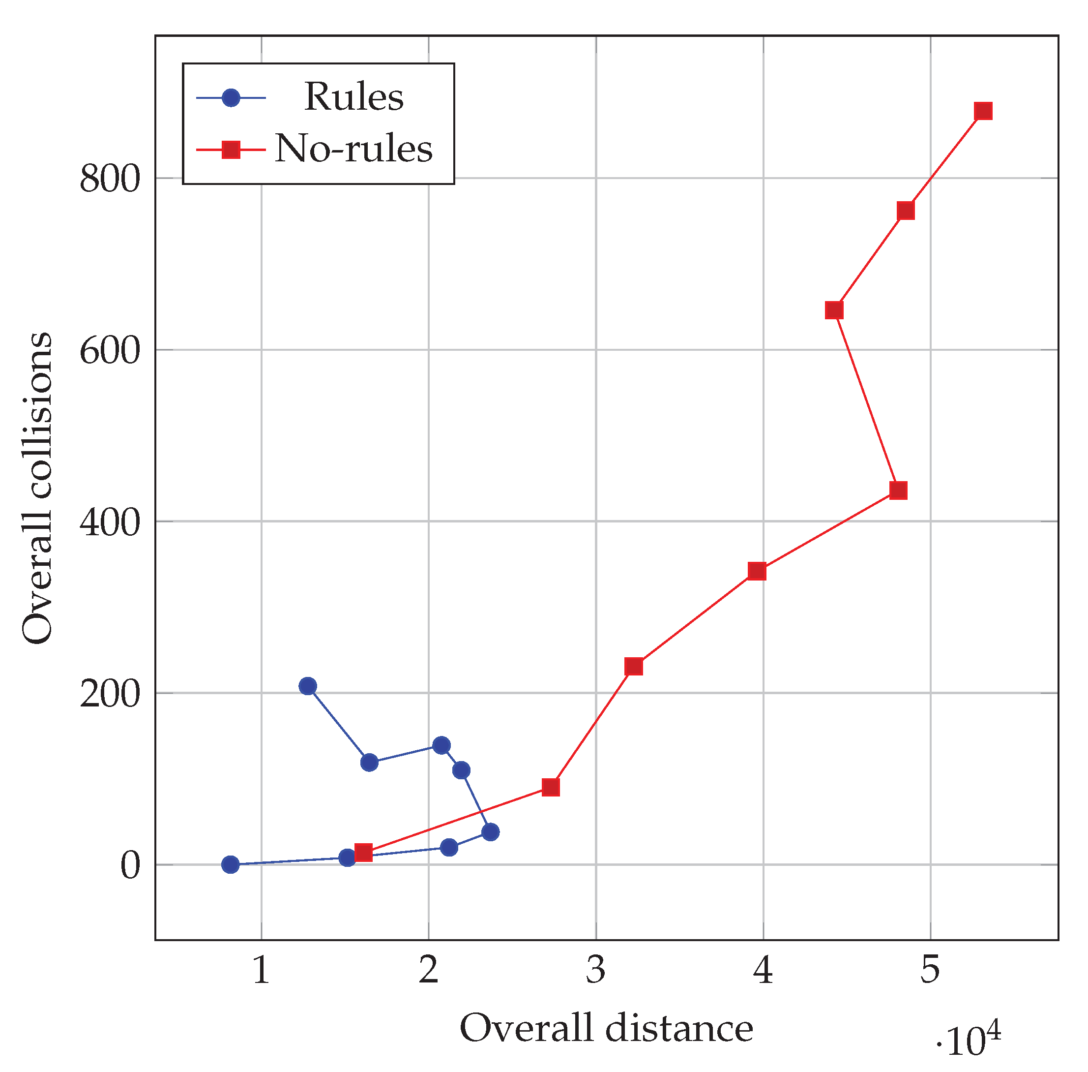
With the aim of investigating the impact of the traffic level on the behavior observed with the learned policies (in the second learning scenario), we performed several other simulations by varying the number of cars in the road graph. Upon each simulation, we measured the overall distance traveled ${\sum }_{i=1}^{n_{\mathrm{car}}}{E}_i\Delta t$ and overall collisions ${\sum }_{i=1}^{n_{\mathrm{car}}}{C}_i$. We considered the overall sums, instead of the average, of these indexes in order to investigate the impact of the variable number of cars in the graph: in principle, the larger is this number, the longer is the overall distance that can be potentially traveled, and, likely, the larger is the number of collisions.

We show the results of this experiment in Figure 6, where each point corresponds to indexes observed in a simulation with a given traffic level $n_{\mathrm{car}}$: we considered values in $10,20,\cdots ,80$. We repeated the same procedure for both the drivers trained with and without the rules, using the same road graph in which the drivers have been trained. For each level of traffic injected, we simulated T time steps and we measured the overall distance and overall number of collisions occurred.

As shown in Figure 6, the two policies (corresponding to learning with and without rules) exhibit very different outcomes as the injected traffic increases. In particular, the policy optimized without rules results in an overall number of collisions that increases, apparently without any bound in these experiments, as the traffic level increases. Conversely, the policy learned with the rules keeps the overall number of collisions much lower also with heavy traffic. Interestingly, the limited increase in collisions is obtained by the policy with the rules at the expense of overall traveled distance, i.e., of traveling capacity of the traffic system.

From another point of view, Figure 6 shows that a traffic system where drivers learned to comply with the rules is subjected to congestion: when the traffic level exceeds a given threshold, introducing more cars in the system does not allow obtaining a longer traveled distance. Congestion is instead not visible (at least not in the range of traffic levels that we experimented with) with policies learned without rules; the resulting system, however, is unsafe. Overall, congestion acts here as a mechanism, induced by rules applied during the learning, for improving the safety of the traffic system.

6. Conclusions

We investigated the impact of imposing traffic rules while learning the policy for AI-powered drivers in a simulated road traffic system. To this aim, we designed a road traffic model that allows analyzing system-wide properties, such as efficiency and safety, and, at the same time, permits learning using a state-of-the-art RL algorithm.

We considered a set of rules inspired by real traffic rules and performed the learning with a positive reward for traveled distance and a negative reward that punishes driving behaviors that are not compliant with the rules. We performed a number of experiments and compared them with the case where rules compliance does not impact on the reward function.

The experimental results show that imposing the rules during learning results in learned policies that gives safer traffic. The increase in safety is obtained at the expense of efficiency, i.e., drivers travel, on average, slower. Interestingly, the safety is also improved after the learning—i.e., when no reward exists, either positive or negative—and despite the fact that, while training, rules are not enforced. The flexible way in which rules are taken into account is relevant because it allows the drivers to learn whether to evade a certain rule or not, depending on the current situation, and no action is prohibited by design: rules stand hence as guidelines, rather then obligation, for the drivers. For instance, a driver might have to overtake another vehicle in a situation in which overtaking is punished by the rules, if this decision is the only one that allows avoiding a forthcoming collision.

Our work can be extended in many ways. One theme of investigation is the robustness of policies learned with rules in the presence of other drivers, either AI-driven or human, who are not subjected to rules or perform risky actions. It would be interesting to assess how the driving policies learned with the approach presented in this study operate in such situations.

From a broader point of view, our findings may be useful in the situations where there is a trade-off between compliance with the rules and a greater good. With the ever increasing pervasiveness of AI-driven automation in many domains (e.g., robotics and content generation), relevance and quantity of these kinds of situations will increase.