Article

A Method to Generate Vector Beams with Adjustable Amplitude in the Focal Plane

by
Alexandru Crăciun
1,2,* and
Traian Dascălu
2,*
1
National Institute for Laser, Plasma and Radiation Physics, Laboratory of Solid-State Quantum Electronics, Atomistilor 409, Magurele 077125, Ilfov, Romania
2
Doctoral School of Physics, University of Bucharest, Atomistilor 405, Magurele 077125, Ilfov, Romania
*
Authors to whom correspondence should be addressed.
Appl. Sci. 2020, 10(7), 2313; https://doi.org/10.3390/app10072313
Submission received: 27 February 2020 / Revised: 23 March 2020 / Accepted: 23 March 2020 / Published: 28 March 2020
(This article belongs to the Special Issue Ultrafast Vortex Pulses)

Abstract

:

Featured Application

Stimulated emission depletion (STED microscopy); control of point-spread function; micromachining; generation of nearly top-hat beams, partially with radial polarization.

Abstract

We design and investigate an original optical component made of a c-cut uniaxial crystal and an optical system to generate cylindrical vector beams with an adjustable polarization state. The original optical component has a specific, nearly conical shape which allows it to operate like a broadband wave retarder with the fast axis oriented radially with respect to the optical axis. We show via numerical simulations, using the Debye–Wolf diffraction integral, that the focal spot changes depending on the polarization state, thus enabling the control of the focal shape. Non-symmetrical shapes can be created although the optical system and incoming beam are circularly symmetric. We explained, using Jones matrix formalism, that this phenomenon is connected with the Gouy phase difference acquired by certain modes composing the beam due to propagation to the focal plane. We present our conclusions in the context of two potential applications, namely, stimulated emission depletion (STED) microscopy and laser micromachining. The optical system can potentially be used for STED microscopy for better control of the point-spread function of the microscope and to decrease the unwanted light emitted from the surroundings of the focal point. We give an analytical expression for the shape of the original component using the aspherical lens formula for the two versions of the component: one for each potential application.

1. Introduction

Helical beams are optical beams characterized by a transversal phase distribution with an additional helical phase term 𝓁 θ. Integer parameter 𝓁 is called topological charge, and, if different from zero, it denotes that there is a discontinuity in the phase map. Polarization state may change with the azimuthal angle around the discontinuity, whereby the resulted beam is called a cylindrical vector beam [1].
Structured light and especially helical beams and cylindrical vector beams are deemed suitable for applications like optical trapping and particle manipulation [2,3,4], stimulated emission depletion (STED) microscopy [5,6], laser micromachining [7], or charged particle acceleration in plasma [8].
Cylindrical vector beams can be produced by selection of radial polarization from a circularly polarized beam using a conical window cut at Brewster angle [9], using microstructured birefringent plates, also known as spatially variant polarization converters [10] or liquid crystal modulators [11]. Liu et al. reported an interferometric optical system that allows full control of the polarization and the shape of the beam [12], with measured efficiency around 50%.
Ciattoni et al. [13] demonstrated that propagation of circularly polarized non-collimated beams through c-cut uniaxial crystals results in the generation of helical beams of ±2 topological charge. Transformation of Gaussian fs-laser beams to single- or double-charge vortex beams using a uniaxial crystal was experimentally proven [14], with efficiency limited to 50% for double-charge beams and 75% for single-charge beams. The dynamics of spin-to-orbital angular momentum conversion in uniaxial crystals was further studied by Brasselet et al. [15]. The interaction of circularly polarized, non-collimated, ring-shaped light beams with a single piece of homogeneous uniaxial medium was demonstrated to shape scalar and vectorial beams with nearly 100% conversion efficiency [16]. It was also shown previously by Khilo et al. [17] that Bessel beams can achieve nearly 100% efficiency of conversion into a helical mode due to propagation along the crystal axis of a uniaxial crystal. Real approximations of Bessel beams are characterized by a conical wavefront and a ring-like intensity pattern in far-field [18]; since conversion efficiency depends only on the angular spectrum of the beam, it is natural to consider that a beam with conical wavefront is ideal for mode conversion in uniaxial crystals.
Flat-top beams can be useful for laser-scribing surface micro-structures, to improve the quantity of energy effectively used for ablation, to avoid damaging the material, and to create a sharper ablated channel [19]. Typical optical systems for generation of flat-top beams are highly sensitive to the shape and width of the incident beam [20] and do not produce a collimated beam; therefore, the flat-top profile changes quickly near the designated plane. Recent studies showed that control of polarization is an important aspect for the improvement of machining efficiency. Results regarding various types of femtosecond cylindrical vector beams used for drilling and scribing in crystalline silicon and fused silica were presented in Reference [7]. The conclusion presented therein was that radial polarization is the best option for drilling, to improve the quality of the boreholes. Furthermore, we observed that circular polarization produces better results than linear polarization.
For STED microscopy, one of the main requirements for the depletion beam is to have zero intensity on the optical axis [21]. Intensity on the optical axis could be different from zero due to the effect of the longitudinal electric field that arises at focusing with high-numerical-aperture (NA) lenses. Azimuthally polarized fields are known to be purely transverse (for example, see Figure 5 in Reference [22] and explanations therein) and, therefore, are often employed for fluorescence microscopy beyond the diffraction limit [6,23] (not necessarily STED). A more common approach for STED depletion beams is to make use of circularly polarized helical beams with non-zero total angular momentum, for which the longitudinal electric field undergoes destructive interference along the optical axis and, therefore, the intensity is zero.
In this work, we present the design and analysis of an optical system, capable of producing cylindrical vector beams with adjustable characteristics in the focal plane. Specifically, the focal spot can be changed from a typical doughnut spot with azimuthal polarization to an extended doughnut spot or a bi-lobed focal spot without circular symmetry, via simple rotation of certain optical elements around the optical axis; moreover, if the focal spot is circularly non-symmetric, then it could be rotated around the optical axis by rotation of certain components. The intensity on the optical axis is always zero; therefore, this system has great potential for STED microscopy.
The main (first) optical layout proposed herein is composed of a spiral phase plate (SPP), a quarter-wave plate (QWP), a half-wave plate (HWP), a component capable of converting a Gaussian beam into a cylindrical vector beam, called a mode converter (MC), a polarization rotator (PR), and an objective lens (L), situated on the light path in the order given by the enumeration. MC is a uniaxial crystal with conical-like shaped surfaces aligned with the crystal axis along the symmetry axis of the system. The QWP is used to achieve elliptical polarization, while the HWP is used to rotate the polarization. The mode converter transforms a circularly polarized beam into a cylindrical vector beam. As explained in the previously mentioned paper [16], the uniaxial crystal works similarly with a wave plate having the fast axis oriented radially (or azimuthally, depending on the properties of the material). If a certain length of the crystal is met, the mode converter will act as a quarter-wave retarder. In this situation, the linear (locally linear) polarization resulting from right circular polarization has the direction oriented at 45° clockwise from the radial direction. Circularly polarized modes of the incoming field on the MC are partially converted to helical modes in such way that the total angular momentum is preserved; thus, after the mode converter and SPP, there will be four distinct beams/modes in the system with different topological charges and polarization states, and each will acquire a different amount of Gouy phase shift [24] due to the propagation to the focal plane. As a result, the diffraction pattern in the focal plane can be very different in comparison with the beam after MC and could even be circularly non-symmetric. The diffraction pattern could be modified by a change in weight of or phase difference between the component modes, which is controlled by the rotation of polarization components QWP and HWP placed before MC. As discussed later, such an optical system could generate a beam with some important features to present (a) a desired polarization state in the focal plane, namely azimuthal or partially azimuthal polarization, (b) zero intensity on the optical axis in the focal plane, and (c) changeable intensity pattern in the focal plane between different configurations.
A second layout of the optical system is also presented, which is capable of producing cylindrical vector beams with nearly top-hat intensity profile in the focal plane based on an idea similar to that presented in Reference [25], i.e., to superimpose two scalar beams with a different profile and orthogonal polarization states.
In the second section, the optical system is presented, as well as the function of the component MC in an ideal case. Jones matrix description of the optical system is also presented in this section. In the third section, we give the expression for the shape of MC interfaces using an aspherical lens formula, we present our simulation results about the characteristics of the focal spot, and we also provide a simple explanation based on Jones calculus. Methods used for the simulation are also presented. We discuss the possible applications of the system in the fourth section. Conclusions are given in the last section.

2. Optical System

We present two different layouts. Variation 1 is designed to produce a beam that achieves azimuthal or nearly azimuthal polarization in the focal plane, with the advantage that the shape of the focal spot can be modified, and an extended or circularly non-symmetric focal spot can be generated. Variation 2 is designed to produce an intensity profile that is nearly uniform in the focal plane, while the polarization is circular near the optical axis and radial near the edge.
The principal component in our optical system is a uniaxial crystal with the crystal axis (CA) aligned parallel with the optical axis, called a mode converter (MC). The longitudinal section view of MC with conical shaped surfaces is shown in Figure 1. Characteristics of MC, aperture diameter D, crystal thickness L, physical angle α, and ray tilt angle inside the crystal α0, which is connected with the refractive index, are represented. MC is considered to be made of sapphire (no = 1.7601, ne = 1.7522). Transparent interfaces of the mode converter are conically shaped in an ideal case, while the description of a more realistic MC is presented in the next section; however, for now, let us assume an ideal case. The first surface modifies a collimated incident beam of light in such a way to produce the wavefront desirable for mode conversion inside the component (conical wavefront). When the beam of light passes through the second surface, it becomes collimated. Due to the specific shape of the interfaces and the birefringent nature of the material used, light propagation through the component induces an exchange between the orbital angular momentum and spin angular momentum of the beam. The efficiency of mode conversion is the fraction η of light energy that is converted into a helical mode. Characteristics of MC are chosen in such a way that the efficiency of the mode conversion is η = 50% for variation 1 of the system and around η ≈ 80% for variation 2 of the system. Fraction η of the energy of the incident beam is transferred to a helical mode having a polarization state that is orthogonal on the input polarization while 1 − η of the energy remains in a non-helical mode with the same polarization state as the incoming beam, thereby preserving the total angular momentum.
The optical system for variation 1 is shown in Figure 2a, while the optical system for variation 2 is shown in Figure 2b. We consider a linearly polarized helical beam with topological charge 𝓁 = −1 and Gaussian intensity profile, at wavelength λ = 800 nm, having 16 mm in diameter, which is supposedly generated using a spiral phase plate (SPP). For variation 2, we consider a simple Gaussian beam with the same characteristics, which did not pass through an SPP. The optical beam encounters a quarter-wave plate (QWP) and becomes elliptically polarized, then encounters a half-wave plate (HWP) that controls the orientation of the polarization ellipse. MC is considered to be after the HWP on the light path 1 m away from the starting point. The thickness of the crystal is 9 mm, and the physical angle of the conical surface is 7° for variation 1 of the system and 7.7° for variation 2. The focusing element is placed 150 mm away from MC. A polarization rotator (PR) that rotates the plane of polarization 45° clockwise is inserted between the MC and focusing element. Polarization optical components QWP, HWP, MC, and PR can actually be placed at any z-coordinate in the system; however, their order on the light path should not be changed. The position of SPP with respect to MC may have a slight influence on the focal spot.
An optical system similar to variation 1 was used by Hao and Leger to experimentally evaluate the longitudinal component of the electric field in the focal plane of a high-numerical-aperture (NA) microscope objective [26]. Hao and Leger used a commercially available radial analyzer, instead of MC, which blocks the radial component and allows the azimuthal component of the circularly polarized incoming field to pass; they also used a combination of two HWPs to produce a polarization rotator. We compare our results to those in Reference [26] in the next section.
Let us consider an incoming field with plane wavefront, which means that it can be represented by a bundle of parallel rays, incident on MC. In this case, each of the refracted rays is situated in a plane common with the optical axis and moves away from the optical axis as the z-coordinate increases. As the ordinary axis is parallel with the optical axis, the extraordinary axis must be radially oriented since it has to perpendicular on the ordinary axis and included in the plane formed by the ordinary axis and ray direction. Therefore, MC could be described by Jones matrix R(θ) J(δ) R(−θ), where R(θ) is a rotation matrix, θ is the rotation angle around the optical axis, and δ is the phase shift between extraordinary and ordinary polarizations, which should be the same for all rays in the case of a perfect conical wavefront.
The effect of MC on an arbitrary field represented using circular polarization states is described by a Jones matrix according to Equation (1), where δ is connected with the length of the crystal L, birefringence of the material, and ray tilt inside the crystal, as described by Equation (2), where kz(e)(ϕ) and kz(o)(ϕ) are respectively the longitudinal part of the extraordinary and ordinary plane-waves tilted at angle ϕ with respect to the optical axis, S is the value of the length along z traveled by the plane-wave indexed by ϕ through the material. The angle ϕ is characteristic for a ray; therefore, it is easy to determine the matrix U for each coordinate in the transversal plane of the beam using the points of intersection between rays and MC. The matrix U was also noted by Brasselet et al. (Equation (3) in Reference [15]), although parameter δ was different because the wavefront considered was spherical.
U ( δ ) = [ cos δ i e 2 i θ sin δ i e 2 i θ sin δ cos δ ] ,
δ = k z ( e ) ( ϕ ) k z ( o ) ( ϕ ) 2 S ( L , α , ϕ ) .
In the case of right circular polarization of the incoming optical Gaussian beam on MC, the transmitted beam would be a combination of a helical mode with topological charge +2 and left circular polarization and a non-helical beam with right circular polarization, but since the incoming beam is characterized by topological charge 𝓁 = −1, the resulting beam is actually a combination of a mode with topological charge +1 and left circular polarization and a mode with topological charge −1 and right circular polarization. Superposition of the two modes generates a cylindrical vector beam characterized by the fact that the direction of polarization is rotated 45° clockwise from the radial direction. The polarization rotator does rotate the plane of polarization 45° clockwise, regardless of the input orientation, thereby producing the azimuthally polarized beam. This particular configuration of variation 1 is called variation 1A throughout the paper. Via rotation of the QWP by 90°, a different focal spot can be obtained. In this case, the beam after SPP and MC is a combination of a helical mode −3 with right circular polarization and a helical mode −1 with left circular polarization. The focal spot produced by this beam is more extended due to the contribution of the helical beam with topological charge −3, and the polarization state is slightly different, but the dark area from the center of the focal spot has a similar extension. This particular case is called variation 1C. Intermediate between these two configurations is variation 1B (linear incoming polarization on MC), which produces a two-lobed spot with a highly elongated dark area in the center. Intermediate A–B configurations produce a small focal spot with an elliptical dark region in the center, whereas intermediate B–C configurations produce a larger focal spot with an elliptical dark region in the center. Rotation of HWP controls the orientation of a circularly non-symmetric focal spot, while rotation of QWP controls the shape of the focal spot. A general Jones vector for the field in the plane of the focusing element is given in Equation (3) and is then particularized for variation 1A (Equation (4) using vertical/horizontal polarization and Equation (5) using circular polarization) and variation 1C (Equation (6) using vertical/horizontal polarization and Equation (7) using circular polarization) of the system.
V l e n s = e i θ R ( 45 ° ) B U ( δ ) B 1 J H W P ( γ ) J Q W P ( φ ) V i n = K ( δ ) J H W P ( γ ) J Q W P ( φ ) V i n .
Angles γ and φ give the orientation of the fast axis of HWP and QWP with respect to the horizontal axis. Matrix B makes the conversion from circular to linear polarization.
K ( δ ) = [ 1 1 1 1 ] [ 1 1 i i ] [ cos δ i e 2 i θ sin δ i e 2 i θ sin δ cos δ ] [ 1 i 1 i ] [ e i θ 0 0 e i θ ] ,
[ V x V y ] l e n s = K ( 45 ° ) [ 1 0 0 1 ] [ 1 0 0 i ] [ 1 1 ] = K ( 45 ° ) [ 1 i ] [ sin θ cos θ ] ,
[ V + V ] l e n s = [ 1 i 1 i ] [ sin θ cos θ ] [ e i θ e i θ ] .
[ V x V y ] l e n s = K ( 45 ° ) [ 1 0 0 1 ] [ 1 0 0 i ] [ 1 1 ] = K ( 45 ° ) [ 1 i ] [ cos θ sin θ ] e 2 i θ ,
[ V + V ] l e n s = [ 1 i 1 i ] [ cos θ sin θ ] e 2 i θ [ e 3 i θ e i θ ] .
The second variation of this system is designed to produce a nearly uniform circular spot. This is similar to variation 1A, although the spiral-phase plate is not present. Without SPP, the focal spot is a superposition between a doughnut-shaped spot and a nearly Gaussian one. If the energy contained in each mode would be equal, then the doughnut spot would be much less intense because the energy would be distributed on a larger area. Therefore, it seems that a more uniformly illuminated spot can be produced if the energy contained in the helical mode is increased. This idea was used to produce beams with similar characteristics in Reference [25], although the method to produce these beams was based on liquid crystal modulators. By increasing the length of the crystal or the physical angle of the conical surface, mode conversion efficiency could be around 80%, which makes the focal spot become top-hat. We see in the next section that an MC with a sharp tip is not physically realizable. Therefore, we designed an MC with an extended rounded tip whose shape tends to be conical near the edges.

3. Numerical Simulations and Results

We simulate the optical system using the spectrum of plane-waves method [27] for propagation between SPP and MC, while using ray tracing for propagation between the front face of MC and rear face of the lens, for evaluation of wavefront aberrations, and for optimization of aspherical shapes of MC interfaces. The Debye–Wolf diffraction integral [28] was used to compute the focal spot. Two different aspherical lenses with NA 0.21 (low NA asphere) and 0.47 (high NA asphere) were used, to differentiate between effects caused by strong focusing and effects which are not caused by strong focusing. A simple Wolfram Mathematica code was written to perform the simulations, which is placed as a supplementary material. We briefly describe the methods used for simulations in the first subsection, while we give the expression for all aspherical surfaces, including both lenses and MC for both variations, in the second subsection, and we present and discuss the results regarding the focal spot in the third subsection.

3.1. Methods Used for Numerical Simulations

The spectrum of plane-waves method is well known, easy to implement, and efficient for beams with nearly plane wavefront in the near-field. It involves Fourier transforming the input signal and adding a phase, in accordance with the dispersion relation of the waves and distance between input and output planes, to determine the output signal. Mathematically, it is described in Equation (8).
V ( r , z ) = V 0 ( r 0 ) exp [ i k 0 2 k 2 z + i k ( r r 0 ) ] d k d r 0 ,
where k0 = ω/c and k is the transversal wave-vector of a plane-wave. We use this formula in the case of variation 1 to simulate the propagation of the beam over the distance 
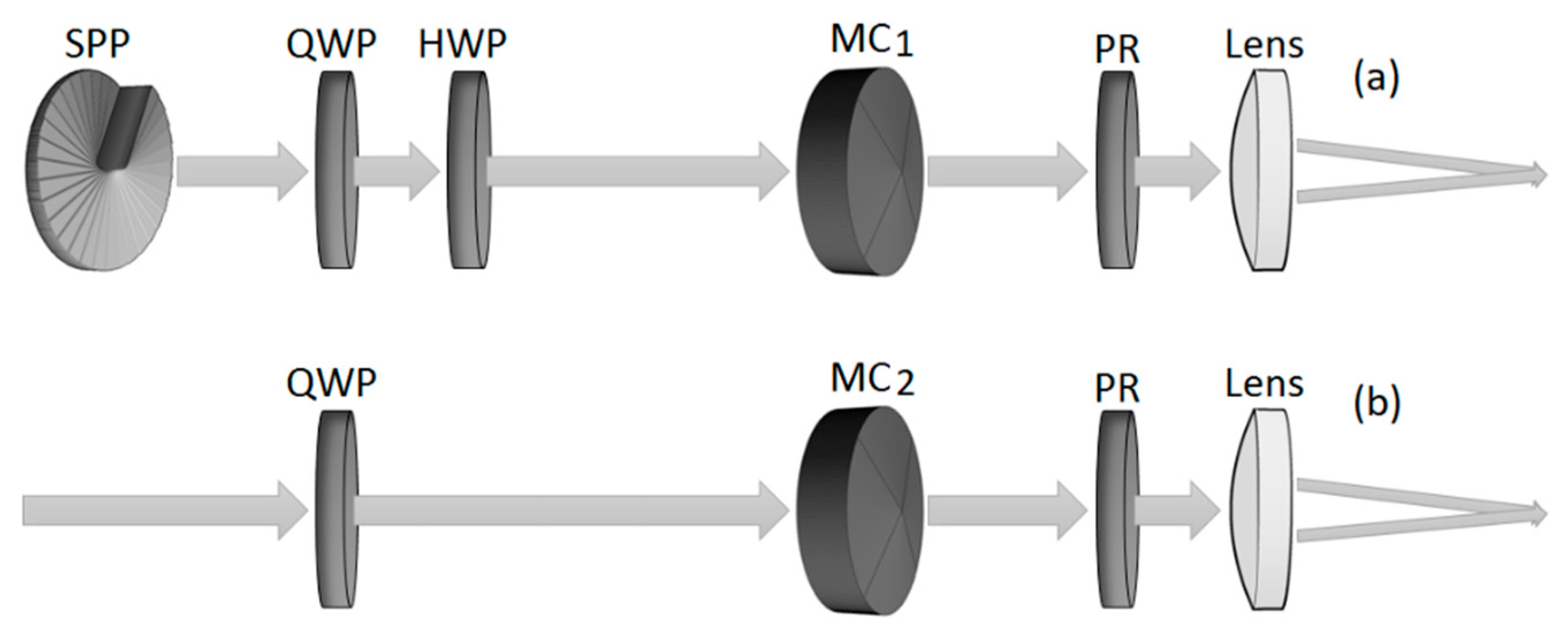
z = 1 m, between SPP and MC, starting with a Gaussian beam with diameter 16 mm, after we multiplied the field with the complex transmission function of SPP (topological charge 𝓁 = −1).
Ray tracing is used everywhere in optics. Therefore, here, we discuss only the way in which we use it to compute the wavefront aberration produced by the combination MC + lens and how we reconstruct the field from ray information traced through an optical component. Firstly, let us define the ray vector (t, tz) which points in the direction of the ray and has the property that k0 t = k. Let us imagine a divergent bundle of rays that originates from a single point. One ray from the bundle intersects a plane surface placed at distance z from the starting point, at coordinate rs(t) = z t/tz, while the optical path length along the ray is s(t) = z/tz. We can observe now that the complex amplitude produced by the plane-wave indexed by k in the plane z, which usually can be written as exp[i kz (k) z + i k·r], where kz (k) = (k20k2)1/2, could also be written as exp[i k0 s(k) + i k·r − i k·rs(k)]. Therefore, we can conclude that information about the ray intersection with the surface and optical path length along the ray can be used to model the propagation of a plane-wave. Now, we have to determine the additional phase that each plane-wave acquires in the focal plan due to the aberrations of the system.
Φ ( k ) = exp [ i k 0 s 1 ( k ) + i k 0 s 2 ( k ) i k r s ( k ) ] exp [ i k 0 s 1 ( k ) + i k 0 2 k 2 f ] .
Equation (9) evaluates the aberrations in the focal plane, usually evaluated in the plane tangent to the rear face of the last component or on the surface of a sphere centered in the focal point. s1(k) is the optical path length along the ray, between the input plane and the plane tangent to the last surface, s2(k) is the optical path length along the ray indexed by k between this plane and the focal plane, and rs is the point of intersection between the ray and the focal plane. The approximate value from Equation (9) is equivalent to the wavefront aberration as is usually employed for the Debye–Wolf integral since it is given up to a constant by the optical path length between the input plane and the sphere of radius f centered in the focal point. We used the correct value from Equation (9), which also takes into consideration that the plane-waves are not directed exactly to the focal point.
To determine the complex amplitude of the beam in a certain plane after the focusing element, in the point indicated by vector R, we simply take the complex amplitude in the input plane, in the point r(R) that gives the intersection between the input plane with the ray which passes through R, and we multiply this value with a factor which accounts for the fact that the density of rays changes along the ray indexed by R. Ray density is computed using a Voronoi mesh [29] as the inverse of the area of a Voronoi cell; Voronoi mesh is a built-in function of Wolfram Mathematica. The complex amplitude of the beam in the output plane (after the lens) is given in Equation (10), where the phase factor exp[i k0 s1(R)] was dropped but is later included when the Debye–Wolf integral is performed, in Φ(t).
V l e n s ( R ) = V ( r   ( R ) ) A ( r   ( R ) ) A l e n s ( R ) .
For implementation of the Debye–Wolf integral, we used Equations (11)–(14) from Reference [30], with wavefront aberration determined according to Equation (9) and the complex amplitude of the beam, denoted by Vlens, determined using Equations (8) and (10). The complex amplitude of the beam in the output plane, in the point R, is proportional to the complex amplitude of the plane-wave with direction given by the ray vector of the ray that passes through R. Since there is a one-to-one correspondence between the position in the transversal plane, after the focusing element, and the transversal projection of ray vector t, we can index the complex amplitude depending on t as shown in Equation (11).
V f o c u s ( r ) = i λ L ( t ) V l e n s ( f t ) t z ( t ) exp [ i Φ   ( t ) + i k 0 t r ] d t .
L ( t ) = [ 1 + t z ( 1 t z ) cos 2 θ ( 1 t z ) sin 2 θ ( 1 t z ) sin 2 θ 2 t z cos θ 1 + t z + ( 1 t z ) cos 2 θ 2 t z sin θ ] .
Matrix , whose expression is in Equation (12), gives the contribution of each plane-wave to the electric field components Ex, Ey, and Ez depending on its polarization, while θ(t) gives the orientation of the ray/plane-wave indexed by t, around the optical axis.

3.2. Expression of the Surface of MC

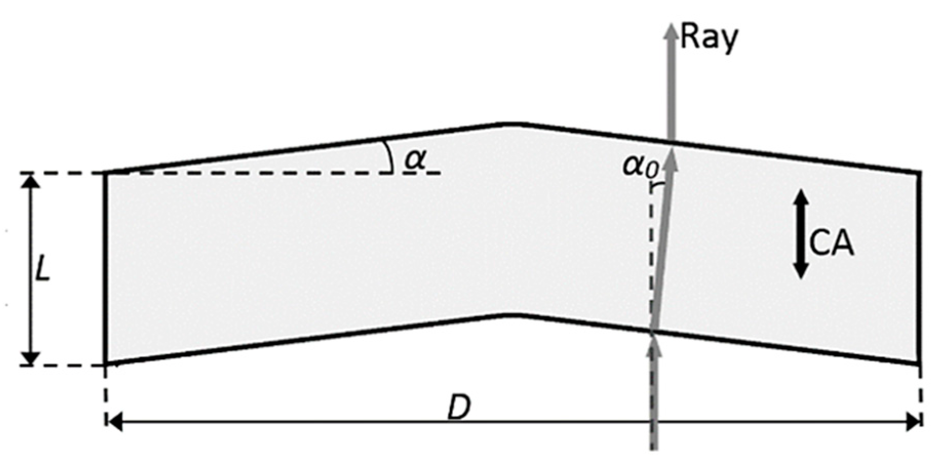
Surfaces of optical component MC should be conical shaped. Although the tip of the rear (convex) face can be produced in practice with enough sharpness, the front (concave face) cannot be made in a conical shape without a non-transmissive region that could be even larger than 2 mm in radius. It seems that a conical (aspherical) shape with a rounded tip and curvature radius larger than 2 mm on the front face will also highly distort the wavefront. The solution we found was to choose a conical (aspherical) shape with a rounded tip with curvature radius 5 mm (for variation 1) and to correct the shape of the rear face using higher aspherical coefficients. We would like to mention that spherical concave lenses with curvature radius less than 5 mm are commercially available. Gonzalez-Acuña and Guitiérrez-Vega [31] determined the shape of the rear surface of a component, being given the equation for the front face, such that the component behaves as an axicon that tilts the rays with angle β. We use these equations by setting β = 0 to determine the shape of the rear surface and then we fit the data using the aspherical lens (Equation (13)).
z ( r ) = r 2 R ( 1 + r 2 R 2 1 ( 1 + κ ) ) + α 2 n r 2 n .
The variation from the target value of mode conversion efficiency of MC for the waves which travel near the optical axis is not essential, in the case of variation 1 all modes are helical; therefore, this will not produce intensity on the optical axis in the focal plane. On the other hand, in the case of variation 2, the mode without topological charge is necessary to form the top-hat shape. Equations for shapes of front/rear interfaces of MC for variation 1 and 2 are presented in Table 1; for completeness, we give also the expression of the front face of the two aspherical lenses used for simulation.
The back surface of MC is designed for an aperture diameter of 26 mm, while the clean aperture is considered 23 mm in diameter. It is very likely that better designs are possible for both versions of MC, while what we present is more a proof of concept. Aspherical coefficients α2n have alternating signs and very high values, which means that they compensate for each other to produce a correction that is not easily described by a polynomial function. As a result, the designed surface presents small variations from the ideal surface, given by equations from Reference [31], which scatter the rays. The geometrical spot for both cases is still sub-wavelength. For version 1 of MC, we could not properly fit the ideal surface near the tip; therefore, the waves that pass through the central region are not focused on the optical axis. MC for variation 2 looks more like a meniscus lens, having a larger curvature radius; therefore, this problem was not present.

3.3. Results

In 
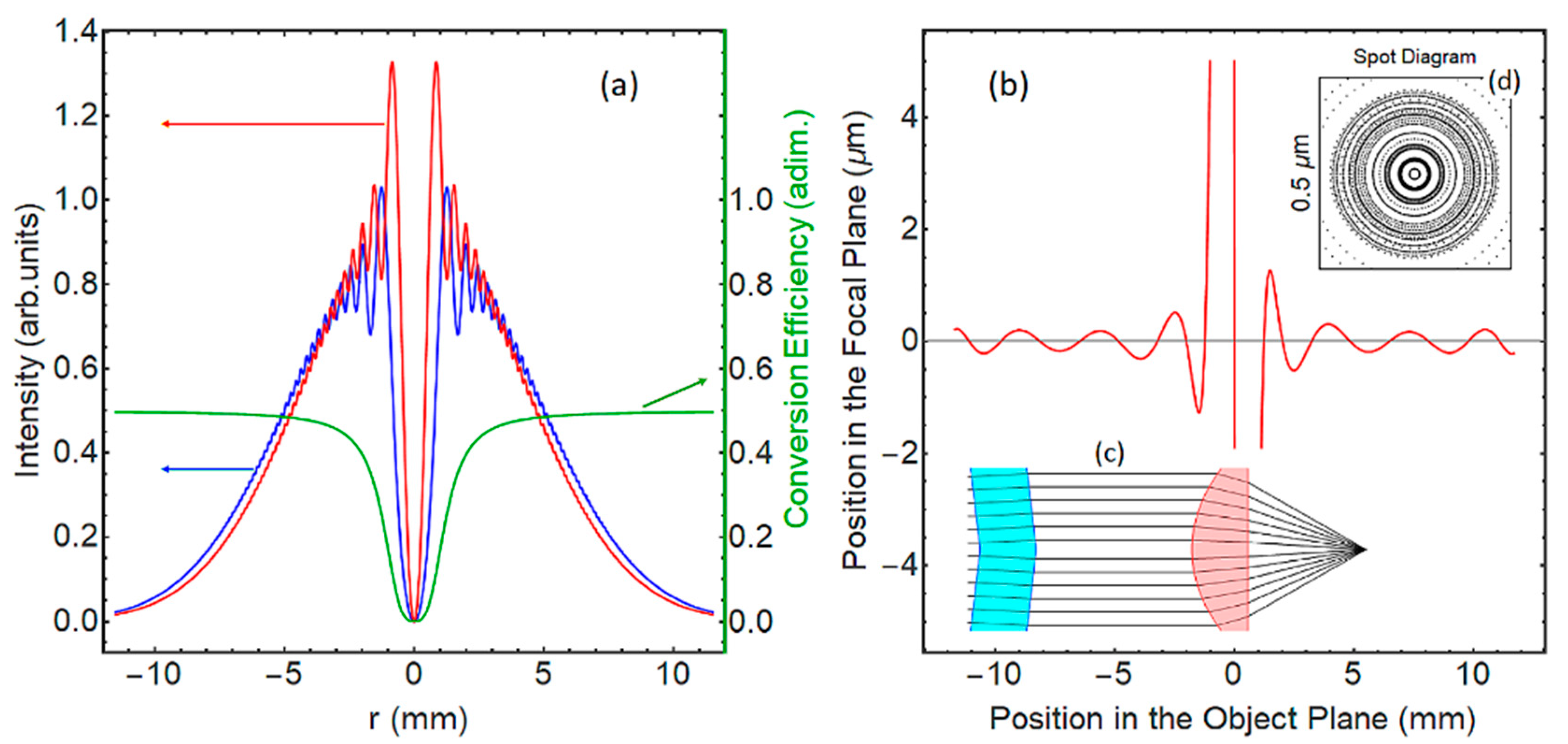
Figure 3a, we show the intensity profile of the beam right before (red) and after (blue) MC for variation 1 of the system, with green representing the conversion efficiency depending on the input coordinate. The beam is helical due to the presence of SPP, placed 1 m before MC. We can observe that the conversion efficiency is nearly 50%, except in the central region, where it is nearly zero. In Figure 3b, we have a ray-fan diagram (red) which represents the position of the ray in the focal plane depending on the position before the MC. We can observe small oscillations near zero that are caused by the inability of aspherical lens formula to perfectly represent the ideal corrected rear surface of MC. In Figure 3c (inset), we represent MC for variation 1 with the high-NA asphere in the longitudinal section, where the distance between components is shrunk to fit in the image. In Figure 3d (inset) is the ray spot diagram of the system, where we can observe that the geometrical spot is smaller than the wavelength and, therefore, the system is nearly diffraction-limited.
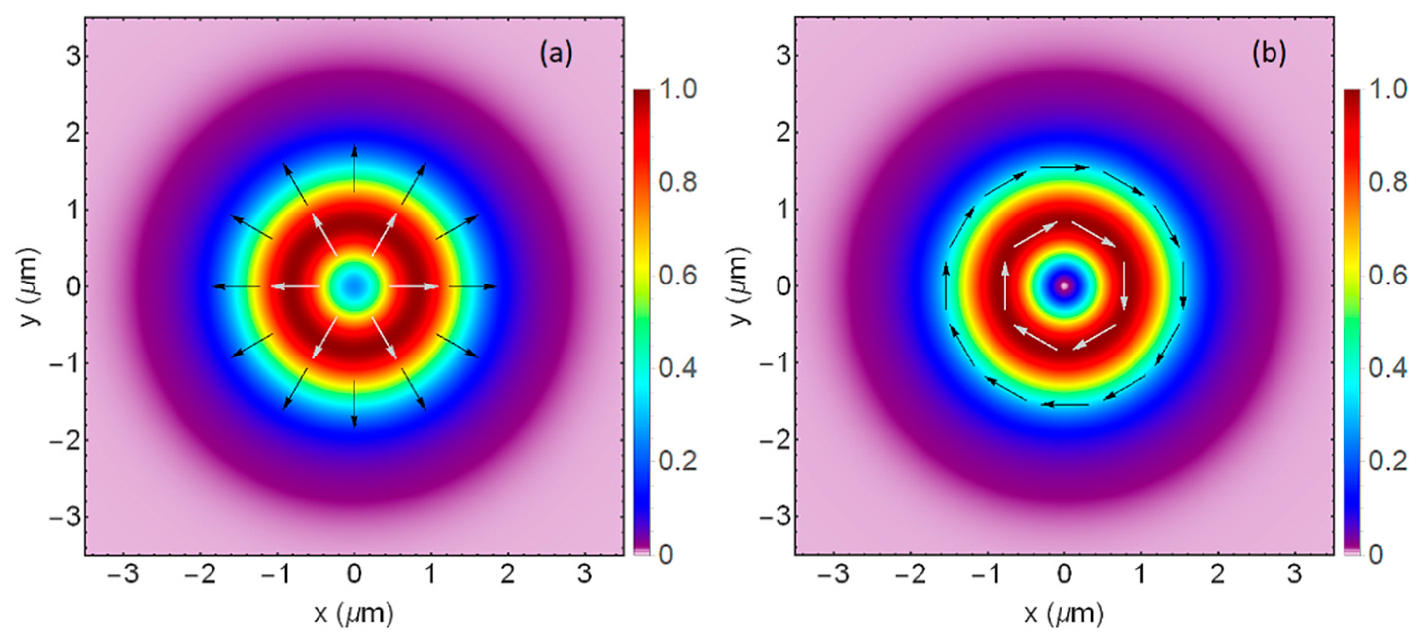
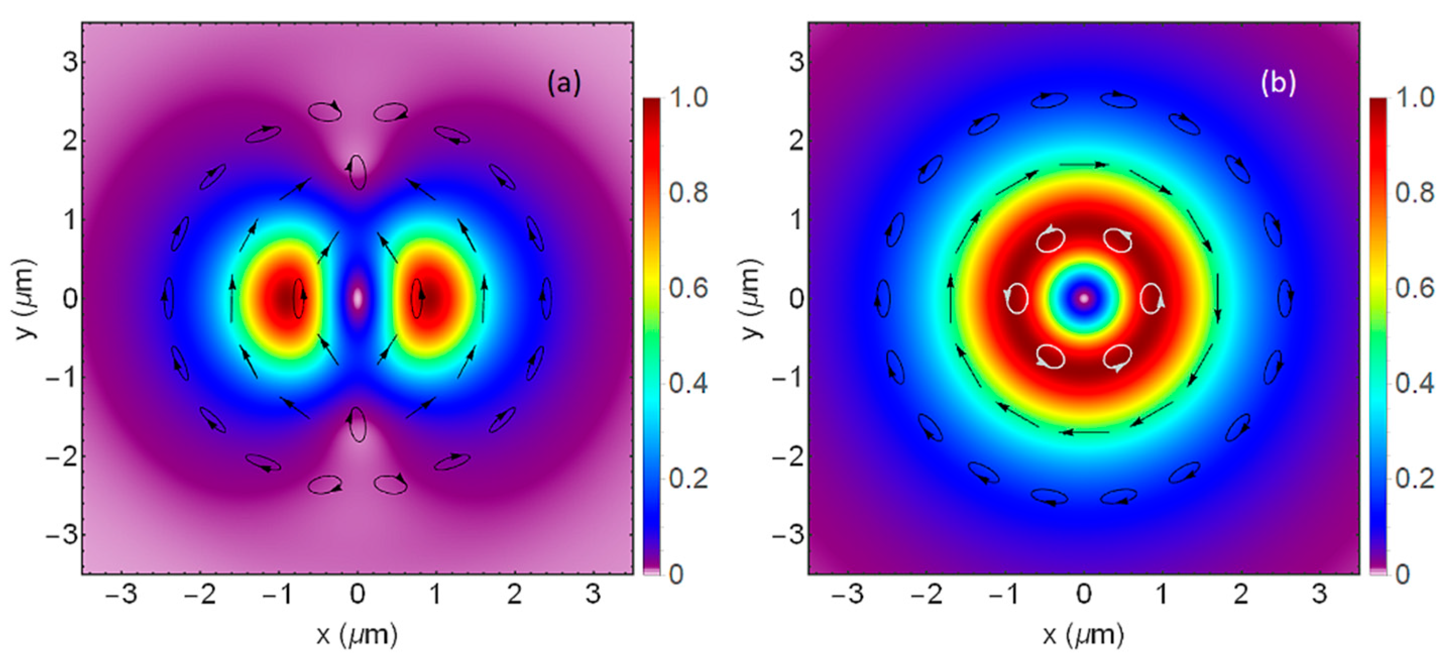
The focal spot for variation 1A, which is polarized azimuthally, is presented in Figure 4b, while a focal spot with radial polarization is presented in Figure 4a for comparison. The radially polarized focal spot can be generated using a polarization rotator that rotates the polarization anti-clockwise instead of clockwise. The high-NA aspherical lens (0.47 NA) was used for focusing, in both cases. For both cases, the polarization state is the same after PR and in the focal plane because the beam is formed by a superposition between two helical beams with topological charge +1 and −1 with orthogonal circular polarization states. For the azimuthally polarized beam (variation 1A), the intensity profile in the focal plane is typical for a beam used for STED microscopy, having zero intensity on the optical axis. The radially polarized focal spot has non-zero intensity on the optical axis, and this behavior is a marker for high NA focusing, as pointed out, for example, in Reference [22]. The presence of longitudinal electric field on the optical axis for the radially polarized helical beams was also experimentally demonstrated in Reference [26]. This is proof that, by using a lens with 0.47 NA, we are in the strong focusing regime. We should observe a non-zero intensity on the optical axis for variation 1B and 1C if this effect is present, and we should be able to determine if the focal spot generated by variation 1B or by variation 1C is proper for STED microscopy.
Focal spots produced by variation 1B and variation 1C using the same focusing element are shown in Figure 5a,b respectively, where the polarization state is also shown. We can observe in Figure 5 that, around 2 μm from the optical axis, polarization becomes azimuthal. This may seem unexpected since the polarization for variation 1C is radial after the polarization rotator (Equations (6) and (7)). This change in polarization state suggests that the phase difference between the two circularly polarized modes that are superimposed increases with π. This phenomenon is attributed to the Gouy phase shift [24], which is different for the mode with topological charge −3. For both cases, the intensity is zero on the optical axis, and, for both cases, the polarization is partially azimuthal. The main difference between the two configurations is that variation 1B produces a focal spot with axial symmetry, while, in the case of variation 1C, the focal spot is circularly symmetric. The focal spot generated by variation 1A is also circularly symmetric but less extended than in the case of variation 1C.
The expression of the complex electric field generated by a paraxial Gauss–Laguerre mode is given in Equation (14), where the only phase term which depends on the z-coordinate and is not common for modes with different indexes is the Gouy phase term ψp𝓁(z) = (2 p + |𝓁| + 1) arctan(z λ/(π w20)). Considering the focal plane as the origin, we can evaluate the Gouy phase in the plane of the lens, with the expression given in Equation (15). Other notations are as follows: w(z) is the z-dependent half-diameter of the beam, q(z) is the complex beam parameter, and Lp|𝓁| is the generalized Laguerre polynomial.
E ( r , z ) = w 0 w ( z ) ( r 2 w ( z ) ) | | L p | | ( 2 r 2 w 2 ( z ) ) exp ( i k 0 r 2 2 q ( z ) + i k 0 z + i θ + i ψ p ( z ) ) .
ψ l e n s = π 2 ( 2   p + | | + 1 ) .
The mode with helical index −3 acquires a phase π with respect to modes with helical index −1, which justifies a change of sign in the Jones vector, as done in Equations (18) and (19).
[ V x V y ] a f t e r H W P = ( ( 1 + i ) [ 1 i ] + ( 1 i ) [ 1 i ] ) e i θ .
[ V + V ] l e n s = [ e i θ e i θ ] [ e 3 i θ e i θ ] [ i e 2 i θ sin θ cos θ ] .
[ V + V ] f o c u s = [ e i θ e i θ ] [ e 3 i θ e i θ ] cos θ [ e 2 i θ 1 ] .
[ V x V y ] f o c u s = [ 1 1 i i ] [ e 2 i θ cos θ cos θ ] e i θ cos θ [ sin θ cos θ ] .
Equations (16)–(19) describes the beam generated by variation 1B, represented in Figure 5a using Jones vectors. For the Jones vector description, we consider an ideal MC; note that input polarization (before QWP) is (1, 1). Equation (16) represents the polarization state after the HWP (before MC), considering HWP oriented with the fast axis along x and QWP oriented at 45°, as a superposition of right/left circularly polarized modes. The Jones vector for the beam in the plane of the lens is given in Equation (17). Equations (18) and (19) give the polarization state in the focal plane. We observe that the cos θ dependence of the complex field amplitude in the focal plane, as well as the nearly azimuthal polarization state, can be explained by a change of sign in the Jones vector for the mode with topological charge −3. Polarization is not perfectly linear with azimuthal orientation because the modes do not have the same amplitude profile. Polarization is linear only in the region where the amplitude of the mode with topological charge −3 is equal to the amplitude of the mode with topological charge −1. This affirmation is correct also for the spot produced by variation 1C, represented in Figure 5b.
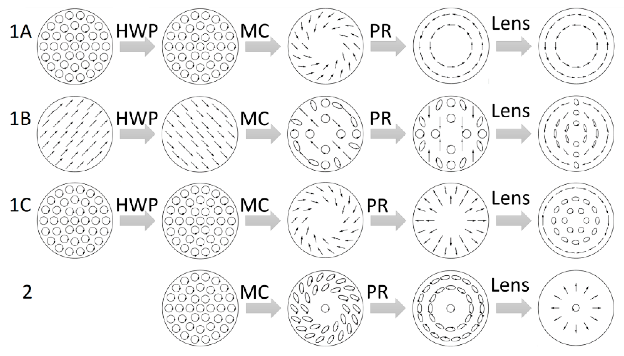
We summarize the polarization states of the beam after each optical component and for each variation of the system 1A, 1B, 1C, and 2 in Figure 6. Variation 2 is the configuration of the system for the generation of flat-top beams. Note that the first polarization state represented is the polarization state of the beam after QWP; note that MC for variation 2 is different from MC for variation 1A, 1B, and 1C, and also note that HWP produces a relevant effect only in the case of variation 1B for which it can be used to rotate the diffraction pattern. For variation 2, the polarization state along the optical axis is maintained through the system.
We also consider the case with QWP and HWP rotated simultaneously in the same direction, with the rotation angle of QWP twice the rotation angle of HWP (φ = 2γ). The Jones vector for the beam after the HWP is given in Equation (20) as a superposition between right and left circularly polarized modes, and we can see that the weight of each mode is controlled by the rotation angle φ of the QWP. As a consequence, the beam in the plane of the lens (expression given in Equation (21)) is described as the summation of one azimuthally polarized beam with zero angular momentum (expression given in Equation (5)) and a radially polarized beam with non-zero angular momentum (with expression given Equation (7)). As we did before, we add a minus sign to the component with topological charge −3 in order to take into account the change in polarization due to propagation to the focal plane; the polarization state in the focal plane is described by Equations (22) and (23).
[ V x V y ] a f t e r H W P = ( sin   φ [ 1 i ] + cos φ [ 1 i ] ) e i θ .
[ V + V ] l e n s = i sin   φ [ e i θ e i θ ] + cos   φ [ e 3 i θ e i θ ] [ e 2 i θ ( i e i θ sin φ + e i θ cos   φ ) i e i θ sin   φ + e i θ cos   φ ] .
[ V + V ] f o c u s = i sin   φ [ e i θ e i θ ] + cos   φ [ e 3 i θ e i θ ] ( i e i θ sin   φ e i θ cos   φ ) [ e 2 i θ 1 ] .
[ V x V y ] f o c u s = ( i e i θ sin   φ e i θ cos   φ ) [ sin θ cos θ ] .
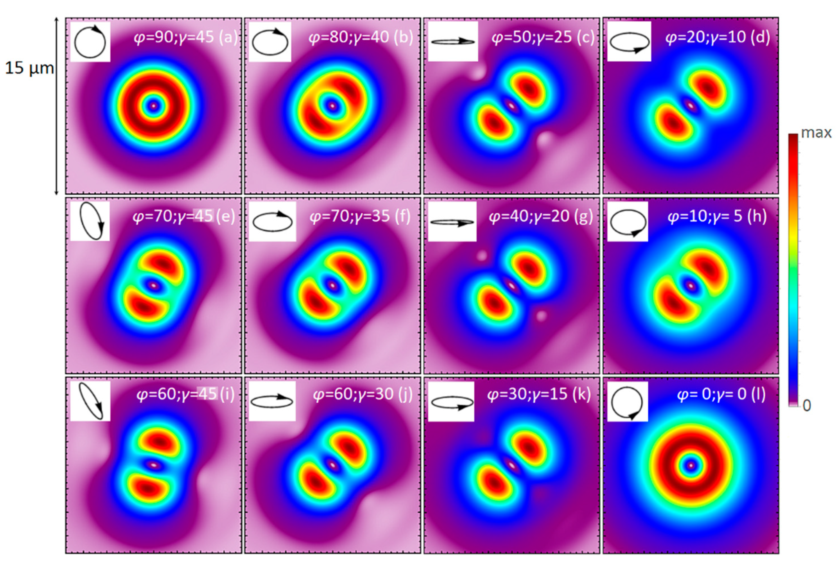
For the simulations presented in Figure 7, we consider the low-NA aspherical lens, with back focal length 46 mm and clear aperture 23 mm in diameter, as the focusing element. Figure 7 also indicates that the phenomenon that leads to the generation of the circularly non-symmetrical focal spot is not due to the strong focusing (presence of Ez component), since the results are in perfect accord with simulations using a focusing element with higher NA, shown in Figure 4 and Figure 5.
In Figure 7a–d,f–h,j–l, we represent the transition between variation 1A and 1C of the system resulting from the clockwise rotation of QWP by 10° and the clockwise rotation of HWP by 5°, which means φ = 2γ; cases φ = 70°, γ = 45° and φ = 60°, γ = 45° are represented in Figure 7e,i, respectively. Rotation of HWP is necessary in order to preserve the orientation of the focal spot and can be used to further control the orientation, which can be observed from the fact that Figure 7e does not have the same orientation as Figure 7f, while Figure 7i does not have the same orientation as Figure 7j. We can see how the polarization state of the beam before MC (represented by black ellipses) affects the focal spot. Results from Figure 7 are well explained by Equation (23).
Hao and Ledger [26] used a similar optical system, using a radial analyzer instead of MC and a polarization rotator that rotated the polarization by 90°. They produced two different types of radially polarized vector beams depending on the input polarization on the radial analyzer. One of the vector beams produced a focal spot similar to that presented in Figure 4a, and the other vector beam produced a focal spot similar to configuration 1C (Figure 5b). They experimentally proved that the radially polarized focal spot possesses non-zero intensity along the optical axis. We wanted to point out that the focal spot which is similar to the focal spot represented in Figure 5b is also radially polarized before the focusing element, and it is likely that the underlying phenomenon that generates this certain focal shape is the same. The configurations that can be produced using elliptical/linear input polarization are not evidenced in the paper, but they are likely to be different from our case since the linearly polarized beam cannot become circularly symmetric after the radial analyzer. Sánchez-López et al. [32] also showed that the Gouy phase plays an important role in the change of the intensity profile of a vector beam near the focal point.
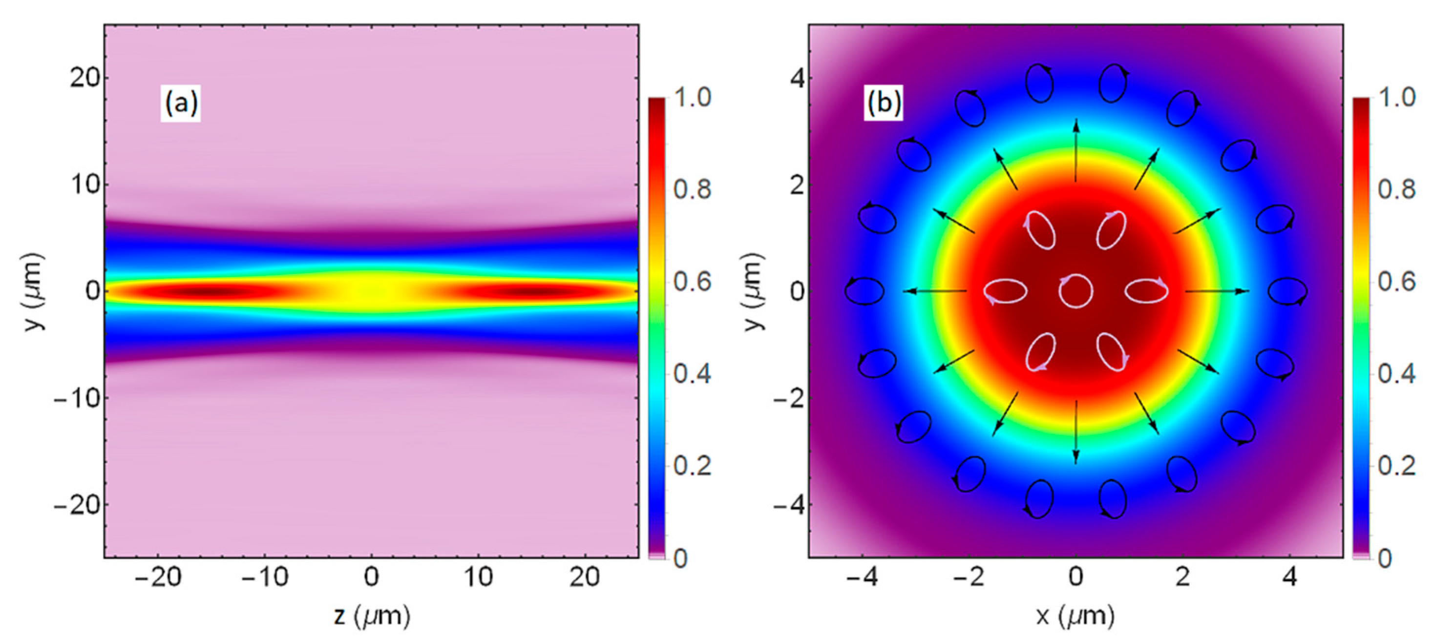
In Figure 8, we show the focal spot produced by variation 2 of the optical system proposed herein. The optical layout is similar to the layout for variation 1A, except that MC has slightly different characteristics and SPP is not present. Unlike variation 1A, the beam is composed of a helical mode −2 with left circular polarization and a non-helical mode with right circular polarization, while the mode conversion efficiency is set around 80%. The profile flatness is good and is maintained for 5–10 µm. The edges are not sharp, but this is not a design problem; it is caused by the fact that the spot is almost diffraction-limited and the length in the transversal plane on which the intensity drops from the maximum value to zero is approximatively given by the radius of the diffraction-limited spot. The polarization state is circular near the optical axis. One of the major advantages is the fact that the spot is radially polarized near the edges of the flat profile; radial polarization, as pointed in Reference [7], is ideal for Si/SiO2 processing, especially for drilling boreholes.

4. Discussion

Here, we explain how this system could be useful for STED. Resolution in STED microscopy is given by the quality of the beams used, their properties, and the ability to detect fewer and fewer photons. There is no fundamental limit for how small the point-spread function (PSF) could be, as in the case of a confocal microscope. Two issues are addressed here. Firstly, optical aberrations could generate pump beam defocusing or determine the two beams not to be perfectly collinear. In any of the cases mentioned above, it is possible that the pump beam partially illuminates a region that is not under the influence of the depletion beam, thus producing an unintended fluorescence light that will decrease the resolution. The spot shown in Figure 5b has a much greater spatial extent, and, in this way, it will decrease the possibility of unwanted fluorescence light. The second problem is the signal-to-noise ratio. Because the fluorescence light originates from a very small volume, very few photons are actually produced; therefore, the signal is weak. Furthermore, the presence of a longitudinal electric field along the optical axis for the depletion beam may decrease the signal [21]. Variation 1B of the system, as well as any configuration intermediate between 1A and 1C, may be useful to increase the signal-to-noise ratio for probe scanning along a line. While intermediate configurations also do not present a longitudinal electric field along the optical axis, the dark region becomes elliptical. This will decrease resolution in one direction, but, at the same time, will allow more photons to be produced.
To place our work in an even broader context, we would like to mention that the MC can be replaced with any component that has the function of a radially symmetrical waveplate with the same retardance. For example, liquid crystal radially symmetric HWPs are commercially available, and radially symmetric QWPs should be readily available if practical applications are found. Since the mode conversion efficiency to a helical beam of a radially symmetric QWP is 50%, probably these were not considered useful. We first conceptualized the idea to generate vector beams with variable polarization state when we studied the potential of uniaxial crystals to generate broadband scalar helical beams and, therefore, we designed this system thinking from this perspective. However, there should be multiple different methods to generate beams with variable polarization using different types of radially symmetric QWP. The advantages of using an MC realized from a uniaxial crystal may be the broadband character and high damage threshold. MC can be realized from various other materials like magnesium fluoride or KDP (potassium di-hydrogen phosphate) and, therefore, uniaxial crystals can be used to generate cylindrical vector beams for a broad range of wavelengths from ultraviolet (UV) to far infrared (IR).
An optical component MC similar to those designed herein could be useful for the generation of scalar helical beams with topological charge ±2 for various applications as long as the parameters are set to result in 100% conversion efficiency (radially symmetric HWP function).

5. Conclusions

In conclusion, we presented an optical component for generation of cylindrical vector beams. This optical component, here named a mode converter, is a c-cut uniaxial crystal with nearly conical-shaped surfaces. The mode converter is embedded in an optical system composed of a QWP, HWP, spiral phase-plate, polarization rotator, and focusing element. We describe the system in a meticulous way and simulate the system using physical optics specific methods.
Variation 1 of the optical system presented is useful to produce beams for STED microscopy characterized by the absence of a longitudinal electric field along the optical axis and good control on the spatial extension, the shape of the focal spot, and its orientation. In other words, a STED microscope based on our system should be capable of controlling the shape and orientation of the PSF. The resolution and signal-to-noise ratio may also be improved.
Variation 2 of the system is useful to produce beams with a nearly flat-top profile in the focal plane, which should be useful for material processing, since the focal spot also possesses partially radial polarization.
When the optical beams produced by this system are focused, an interesting phenomenon is observed. Simulations show that, in the case of a linear incoming polarization state on MC, the focal spot loses the circular symmetry and becomes elliptical. We explained this effect based on the Gouy phase difference acquired by the component of the laser field with topological charge −3 due to the propagation to the focal plane.

6. Patents

Craciun, A.; Dascalu, T. Sistem Optic pentru Producerea de Fascicule Optice Elicolidale Vectoriale. Patent Application submitted to Romanian State Office for Inventions and Trademarks, nr. A/00657, 17.10.2019.

Supplementary Materials

A simple Wolfram Mathematica code placed inside a Mathematica notebook is available online at https://www.mdpi.com/2076-3417/10/7/2313/s1, which also contains some examples, comments, and supplementary figures.

Author Contributions

Conceptualization, A.C. and T.D.; investigation, A.C.; software, A.C.; supervision, T.D.; writing—original draft, A.C.; writing—review and editing, T.D. All authors have read and agreed to the published version of the manuscript.

Funding

This work was supported by a grant of Ministry of Research and Innovation, CNRS-UEFISCDI, project PN-III-P4-ID-PCCF-2016-0164, within PNCDI III and partially financed by Program NUCLEU-LAPLAS VI under grant agreement 16N/2019.

Acknowledgments

The authors greatly appreciate the support and suggestions received from Nicolaie Pavel.

Conflicts of Interest

The authors declare no conflict of interest.

References

  1. Zhan, Q. Cylindrical vector beams: From mathematical concepts to applications. Adv. Opt. Photonics 2009, 1, 1–57. [Google Scholar] [CrossRef]
  2. Skelton, S.E.; Sergides, M.; Saija, R.; Iatì, M.A.; Maragó, O.M.; Jones, P.H. Trapping volume control in optical tweezers using cylindrical vector beams. Opt. Lett. 2013, 38, 28–30. [Google Scholar] [CrossRef] [PubMed]
  3. Jeffries, G.D.M.; Edgar, J.S.; Yiqiong, Z.; Shelby, J.P.; Christine, F.; Chiu, D.T. Using polarization-shaped optical vortex traps for single-cell nanosurgery. Nano Lett. 2007, 7, 415–420. [Google Scholar] [CrossRef] [PubMed] [Green Version]
  4. Zhang, H.; Lizana, A.; Van Eeckhout, A.; Turpin, A.; Ramirez, C.; Iemmi, C.; Campos, J. Microparticle manipulation and imaging through a self-calibrated liquid crystal on silicon display. Appl. Sci. 2018, 8, 2310. [Google Scholar] [CrossRef] [Green Version]
  5. Mller, T.; Schumann, C.; Kraegeloh, A. STED Microscopy and its applications: New insights into cellular processes on the nanoscale. Chemphyschem 2012, 13, 1986–2000. [Google Scholar] [CrossRef] [PubMed]
  6. Xue, Y.; Kuang, C.; Li, S.; Gu, Z.; Liu, X. Sharper fluorescent super-resolution spot generated by azimuthally polarized beam in STED microscopy. Opt. Express 2012, 20, 17653–17666. [Google Scholar] [CrossRef]
  7. Hnatovsky, C.; Shvedov, V.G.; Krolikowski, W. The role of light-induced nanostructures in femtosecond laser micromachining with vector and scalar pulses. Opt. Express 2013, 21, 12651–12656. [Google Scholar] [CrossRef]
  8. Luis Martins, J.; Vieira, J.; Ferri, J.; Fülöp, T. Radiation emission in laser-wakefields driven by structured laser pulses with orbital angular momentum. Sci. Rep. 2019, 9, 9840. [Google Scholar] [CrossRef] [Green Version]
  9. Kozawa, Y.; Sato, S. Generation of a radially polarized laser beam by use of a conical Brewster prism. Opt. Lett. 2005, 30, 3063–3065. [Google Scholar] [CrossRef] [PubMed]
  10. Beresna, M.; Kazansky, P. Space Variant Polarization Converter. US Patent 10156669B2, 3 May 2012. [Google Scholar]
  11. Chen, P.; Lu, Y.-Q.; Hu, W. Beam shaping via photo patterned liquid crystals. Liq. Cryst. 2016, 43, 2051–2061. [Google Scholar] [CrossRef]
  12. Liu, S.; Qi, S.; Zhang, Y.; Li, P.; Wu, D.; Han, L.; Zhao, J. Highly efficient generation of arbitrary vector beams with tunable polarization, phase, and amplitude. Photonics Res. 2018, 6, 228–233. [Google Scholar] [CrossRef]
  13. Ciattoni, A.; Cincotti, G.; Palma, C. Circularly polarized beams and vortex generation in uniaxial media. J. Opt. Soc. Am. A 2003, 20, 163–171. [Google Scholar] [CrossRef]
  14. Shvedov, V.G.; Hnatovsky, C.; Krolikowski, W.; Rode, A.V. Efficient beam converter for the generation of high-power femtosecond vortices. Opt. Lett. 2010, 35, 2660–2662. [Google Scholar] [CrossRef] [PubMed]
  15. Brasselet, E.; Izdebskaya, Y.V.; Shvedov, V.G.; Desyatnikov, A.S.; Krolikowski, W.; Kivshar, Y.S. Dynamics of optical spin-orbit coupling in uniaxial crystals. Opt. Lett. 2009, 34, 1021–1023. [Google Scholar] [CrossRef]
  16. Loussert, C.; Brasselet, E. Efficient scalar and vectorial singular beam shaping using homogeneous anisotropic media. Opt. Lett. 2010, 35, 7–9. [Google Scholar] [CrossRef]
  17. Khilo, N.A. Diffraction and order conversion of Bessel beams in uniaxial crystals. Opt. Commun. 2012, 5, 503–509. [Google Scholar] [CrossRef]
  18. McGloin, D.; Dholakia, K. Bessel beams: Diffraction in a new light. Contemp. Phys. 2005, 46, 15–28. [Google Scholar] [CrossRef]
  19. Rung, S.; Barth, J.; Hellmann, R. Characterization of laser beam shaping optics based on their ablation geometry of thin films. Micromachines 2014, 5, 943–953. [Google Scholar] [CrossRef]
  20. Hoffnagle, J.A.; Shealby, D.N. Optical and mechanical tolerances for two-lens plano-aspheric laser beam shapers. Proc. SPIE 2012, 8490, 849004. [Google Scholar]
  21. Galiani, S.; Harke, B.; Vicidomini, G.; Lignani, G.; Benfenati, F.; Diaspro, A.; Bianchini, P. Strategies to maximize the performance of a STED microscope. Opt. Express 2012, 20, 7362–7374. [Google Scholar] [CrossRef]
  22. Youngworth, K.; Brown, T.G. Focusing of high numerical aperture cylindrical-vector beams. Opt. Express 2000, 7, 77–87. [Google Scholar] [CrossRef] [PubMed]
  23. Gu, M.; Kang, H.; Li, X. Breaking the diffraction-limited resolution barrier in fiber-optical two-photon fluorescence endoscopy by an azimuthally-polarized beam. Sci. Rep. 2014, 4, 3627. [Google Scholar] [CrossRef] [PubMed]
  24. Feng, S.; Winful, H.G. Physical origin of the Gouy phase shift. Opt. Lett. 2001, 26, 485–487. [Google Scholar] [CrossRef] [PubMed] [Green Version]
  25. Han, W.; Cheng, W.; Zhan, Q. Flattop focusing with full Poincaré beams under low numerical aperture illumination. Opt. Lett. 2011, 36, 1605–1607. [Google Scholar] [CrossRef] [PubMed]
  26. Hao, B.; Leger, J. Experimental measurement of longitudinal component in the vicinity of focused radially polarized beam. Opt. Express 2007, 15, 3550–3556. [Google Scholar] [CrossRef]
  27. Sherman, G. Introduction to the angular-spectrum representation of optical fields. Proc. SPIE 1982, 358, 31–38. [Google Scholar]
  28. Wolf, E.; Gabor, D. Electromagnetic diffraction in optical systems—I. An integral representation of the image field. Proc. R. Soc. Lond. 1997, 253, 349–357. [Google Scholar]
  29. Aurenhammer, F. Voronoi diagrams—A survey of a fundamental geometric data structure. ACM Comput. Surv. 1991, 23, 345–405. [Google Scholar] [CrossRef]
  30. Foreman, M.R.; Sherif, S.S.; Munro, P.R.; Török, P. Inversion of the Debye-Wolf diffraction integral using an eigenfunction representation of the electric fields in the focal region. Opt. Express 2008, 16, 4901–4917. [Google Scholar] [CrossRef] [Green Version]
  31. Gonzalez-Acuña, R.G.; Guitiérrez-Vega, J.C. Generalization of the axicon shape: The gaxicon. J. Opt. Soc. Am. A 2018, 35, 1915–1918. [Google Scholar] [CrossRef]
  32. Sánchez-López, M.M.; Davis, J.A.; Moreno, I.; Cofré, A.; Cottrell, D.M. Gouy phase effects on propagation of pure and hybrid vector beams. Opt. Express 2019, 27, 2374–2386. [Google Scholar] [CrossRef] [PubMed]
Figure 1. Longitudinal section through the mode converter.
Applsci 10 02313 g001
Figure 2. Schematic representation of the optical system corresponding to variation 1 (a); schematic representation of the optical system corresponding to variation 2 (b).
Applsci 10 02313 g002
Figure 3. The intensity profile before mode converter (MC) is shown in red, the intensity profile after MC is shown in blue, and the conversion efficiency is shown in green (a); the ray-fan diagram is shown in red (b); the MC and aspherical lens, with ray-tracing, in longitudinal section view (c); ray intersection with the focal plane (d).
Applsci 10 02313 g003
Figure 4. Radially polarized focal spot (a); azimuthally polarized focal spot, generated by variation 1A (b).
Applsci 10 02313 g004
Figure 5. Focal spot generated by variation 1B (a); focal spot generated by variation 1C (b).
Applsci 10 02313 g005
Figure 6. Polarization state after each optical component, for each variation of the system.
Applsci 10 02313 g006
Figure 7. Intensity profile in the focal plane for variation 1 of the system, using the aspheric lens with lower numerical aperture. Variation 1A (a), variation 1C (l), and intermediate configurations (bk).
Applsci 10 02313 g007
Figure 8. Intensity profile near the focal plane for variation 2 of the system, using the aspheric lens with the lower numerical aperture (a); intensity profile and polarization state in the focal plane (b).
Applsci 10 02313 g008
Table 1. A detailed description of all surfaces employed in the simulation using the aspherical lens formula.
MC1-FrontMC1-RearMC2-FrontMC1-RearA1-0.21NAA2-0.47NA
R5 mm7.45 mm19.15 mm14.42 mm25.560 mm18.651 mm
κ−67.33−54.74−55.7−14.6−1.01−1.408
cen. thickness9 mm9 mm6 mm9 mm
α2 0.002076 0.01293
α4−0.00003008−0.000094893.270 × 10−61.4755 × 10⁻⁵
α64.857 × 10−79.713 × 10−77.720 × 10⁻¹⁰−5.557 × 10⁻⁹
α8−5.705 × 10⁻⁹−8.430 × 10−91.630 × 10−13−3.511 × 10⁻¹²
α104.446 × 10−115.312 × 10⁻¹¹
α12−2.158 × 10⁻¹³−2.207 × 10⁻¹³
α145.879 × 10−165.343 × 10⁻¹⁶
α16−6.843 × 10⁻¹⁹−5.668 × 10⁻¹⁹
n@800 nm1.76011.76011.51081.7761
MC1 – the mode converter for variation 1, MC2 – the mode converter for variation 2, A1 – the aspherical lens with low NA, A2 – the aspherical lens with high NA.

