Article

Development and Assessment of a Sensor-Based Orientation and Positioning Approach for Decreasing Variation in Camera Viewpoints and Image Transformations at Construction Sites

1
Department of Civil, Architectural & Environmental Engineering, Drexel University, Philadelphia, PA 19104, USA
2
Rinker School of Construction Management, University of Florida, Gainesville, FL 32611, USA
*
Author to whom correspondence should be addressed.
Appl. Sci. 2020, 10(7), 2305; https://doi.org/10.3390/app10072305
Submission received: 1 February 2020 / Revised: 9 March 2020 / Accepted: 18 March 2020 / Published: 27 March 2020
(This article belongs to the Special Issue Augmented Reality, Virtual Reality & Semantic 3D Reconstruction)

Abstract

:

Featured Application

In this paper, we propose a position and orientation approach that reduces the image transformation phenomena in advance (i.e., process modification). Thus, this approach which integrates with image matching techniques that have limitations dealing with image transformation (i.e., result modification) could be valuable. The advantage of this approach is that it is not dependent on scene features, and therefore it can be used in situations where the features in a scene change or when extremely image transformations occur. This approach can be used as a supplementary approach to assist the feature-based methods.

Abstract

Image matching techniques offer valuable opportunities for the construction industry. Image matching, a fundamental process in computer vision, is required for different purposes such as object and scene recognition, video data mining, reconstruction of three-dimensional (3D) objects, etc. During the image matching process, two images that are randomly (i.e., from different position and orientation) captured from a scene are compared using image matching algorithms in order to identify their similarity. However, this process is very complex and error prone, because pictures that are randomly captured from a scene vary in viewpoints. Therefore, some main features in images such as position, orientation, and scale of objects are transformed. Sometimes, these image matching algorithms cannot correctly identify the similarity between these images. Logically, if these features remain unchanged during the picture capturing process, then image transformations are reduced, similarity increases, and consequently, the chances of algorithms successfully conducting the image matching process increase. One way to improve these chances is to hold the camera at a fixed viewpoint. However, in messy, dusty, and temporary locations such as construction sites, holding the camera at a fixed viewpoint is not always feasible. Is there any way to repeat and retrieve the camera’s viewpoints during different captures at locations such as construction sites? This study developed and evaluated an orientation and positioning approach that decreased the variation in camera viewpoints and image transformation on construction sites. The results showed that images captured while using this approach had less image transformation in contrast to images not captured using this approach.

1. Introduction

Formally, the era of computer vision started in the early 1970s [1]. Computer vision is defined as a trick “to extract descriptions of the world from pictures or sequences of pictures” [2]. This technique assists humans in “making useful decisions about real physical objects and scenes based on images” [3]. According to Horn et al. [4], computer vision “analyzes images and produces descriptions that can be used to interact with the environment”. In summary, the goal of computer vision is “to describe the world that we see in one or more images and to reconstruct its properties, such as shape, illumination, and color distributions” [1]. One of the fundamental processes in computer vision is called image matching [5]. Image matching is “the process of bringing two images geometrically into agreement so that corresponding pixels in the two images correspond to the same physical region of the scene being imaged” [6]. In other words, during the image matching process, two images that are randomly captured from a scene are compared in order to identify their similarity. “Fast and robust image matching is a very important task with various applications in computer vision.” [7]. The process of image matching is required for tracking targets [8], image alignment and stitching [9,10], reconstruction of three-dimensional (3D) models from images [11], object recognition [12], face detection [13,14], data mining [15], robot navigation [8], motion tracking [16,17], and more. These applications are promising in real world problems, and it is possible to leverage them at construction sites to monitor various activities.

1.1. Image Matching Applications in the Construction Industry

In the construction industry, especially in recent years, image matching techniques have shown capabilities for addressing different issues regarding information management. There is abundant research regarding applications of image matching techniques through AEC/FM (architecture, engineering and construction and facilities management). For instance, to solve issues related to difficulties in updating as-built and as-is information on jobsites, some researchers have utilized image matching techniques to create a building information model of the scenes. They have taken images from different angles, stitched them, and attached the data to these models [12]. Others such as Kang et al. [18] reported that in a large-scale indoor environment full of self-repetitive visual patterns, recognizing the location of images captured from different scenes can be confusing. To address this issue, they applied image matching techniques, which analyzed unique features in captured images, to retrieve the location. Kim et al. [19] used image matching techniques to compare virtual images of a construction site with the real construction photographs for the purpose of detecting differences between the actual and planned conditions of the jobsite. Another application of using image matching techniques is to detect changes in a scene by comparing features of pictures captured at different times [20] to estimate the rough progress of a project.
Providing easier access to construction information on a jobsite is another reason to use image matching techniques. For this purpose, some researchers suggested using augmented reality technology to superimpose a layer of data (e.g., text, voice, 3D model, image, etc.) over the locations where access to information is required [21,22]. Marker-based augmented reality (AR) and markerless AR, which both use image matching techniques, can be used for this purpose. For both methods, the image matching algorithms need to detect distinct features between live video frames that are captured from the environment, and a reference image that is already available. In the marker-based approaches, since the algorithms need to detect the features of a label (e.g., Quick Response Code/QR code), the results are very robust [1] in contrast with markerless AR, which needs to use the natural features of the environment that can vary [23,24] (more information regarding AR is presented in Appendix A).

1.2. Problem Statement

In general, there are three main types of algorithms for image matching. The first type is shape matching algorithms, which look for similarities in the shapes of objects in the images [5]. The second type is pixel matching algorithms, which look for similarities in the pixel’s intensity [5]. The third type is called feature-based matching algorithms [5]. In this type, the algorithm detects the distinct local features of images, such as corresponding points, lines, and areas [5].
The challenge these algorithms need to deal with is the variation in the context of pictures that were captured from a scene from different viewpoints. When two pictures are not taken from the same viewpoint, the position, orientation, and scale of the features (e.g., objects and background) in the scene are transformed. Thus, these algorithms should detect the similarities between the features that have been displaced and deformed in the images, and then match them.
In previous decades, to deal with these issues of extracting features, researchers have proposed many different techniques. Some of these techniques detect image features regardless of transformations (e.g., translation and rotation) and illumination but not scaling. This group of techniques is known as single-scale detectors. Techniques such as Moravec detector [25], Harris detector [26], SUSAN detector [27], FAST detector [28,29], and Hessian detector [30,31] are examples of single-scale detectors. Other techniques known as multiscale detectors, including Laplacian of Gaussian [32], difference of Gaussian [33], Harris–Laplace [34], Hessian–Laplace [35], and Gabor–Wavelet detector [36] were later created. In addition to rotation, translation, and illumination, these techniques consider the impact of uniform scaling in detecting features, with the assumption that scale is not affected by an affine transformation of the image structures. Thus, to be able to detect the image features as accurately as possible, it was necessary to create techniques that could handle non-uniform scaling (change in scaling in different directions). Scale invariant feature transform (SIFT) is one of the most advanced versions of these algorithms [1]. SIFT can detect and describe image features [1]. In the first step, the SIFT algorithm detects the local distinct points on images. In the second step, these distinct points (keypoints) are converted into histogram vectors based on the image gradient of each point called keypoint descriptors. SIFT gives value to each of these vectors. In the third step, SIFT compares these values to match the keypoints. However, this is not the end of the process, as not all matches conducted by SIFT are correct. There could be some keypoints in two images with equal values but related to different parts of the scene. For instance, a keypoint on the top of a scene could have equal value with a point on the bottom of a scene. In this case, SIFT cannot distinguish between them. Therefore, incorrect matching occurs. These incorrect matches need to be filtered. For the purpose of filtering the incorrect matches, the fourth step is required. In this step, a technique called RANSAC or random sample consensus [37] is widely used. This approach divides the corresponding points into inlier and outlier sets and finds the best portion of points in inlier sets. To ensure this occurs, first, this algorithm randomly samples two keypoints. The width of the inlier boundary is already determined for this algorithm. RANSAC counts what fractions of points are located inside of this inlier boundary. This process is repeated several times for different keypoints. The largest number of points found as inlier is defined as the best matching pattern, and other matches are removed. Figure 1 illustrates the procedures that SIFT detects, describes, and matches the key points, while RANSAC filters incorrect matches.
However, image matching algorithms are not fully successful when image transformation occurs and image viewpoint changes [5,7,38,39,40]. In fact, increased changes in the image viewpoint can make the matching process unreliable, since the similarity between objects shown on images reduces [5]. For example, an image matching algorithm such as SIFT only works well when the difference between view angles is less than 30 degrees [41]. In addition, if the scaling is too high, the algorithm cannot detect the key points on the frame and the image matching process does not work correctly. For example, three images from a scene are illustrated in Figure 2. The first image (Figure 2a) is the reference image captured. The second image (Figure 2b) is the current frame from the same scene but impacted by the rotation of the camera (more than 30 degrees). The third image (Figure 2c) is also from the same scene but is impacted by high scaling. These scenarios can impact cases such as those using markerless AR that use SIFT and RANSAC during the image matching process. Thus, the algorithm cannot correctly match the features between two images. In addition, when image transformations take place, unrelated and unwanted areas around the scene are also detected. In this situation, change detection algorithms [42] report these areas as a change in the scene. This result is not accurate in construction scenarios where change detection algorithms are used to detect the construction progress based on changes in the image frames.
In addition to the difficulties posed by image transformation, there is another scenario whereby image matching techniques could fail. For example, when a scene is completely changed during a renovation project, the image matching algorithms cannot match the distinct feature points between two frames (e.g., before and after renovation), therefore, the image matching cannot occur. Figure 3 shows a scene that is completely changed before and after renovation. This scenario can impact markerless AR.
Another scenario in which image matching techniques fail to work accurately is when features in two scenes within a location (e.g., a room) are exchanged during renovation. For instance, before renovation, the reference images were captured from the west wall and north wall. During renovation, the features of the west wall and north wall were switched. Since a feature-based system can only detect environmental features and cannot interpret geographical directions, an image matching technique such as SIFT would fail to generate accurate results during the image matching process. To have a clear understanding of this scenario, two scenes have been sketched, as shown in Figure 4. Figure 4a shows a scene before renovation, a door is attached to the west wall, and a window is attached to the north wall. Figure 4b shows the same room, but this time the window has been moved to the west wall and the door has been moved to the north wall. In fact, feature-based tracking methods detect environmental features but not directions. This scenario can impact use cases like markerless AR and change detection.
These limitations of the image matching process motivated us to study supplementary ways (e.g., controlling the image capturing process) to support the image matching algorithms in order to prevent sole dependency on natural features in the scene.

1.3. Ways to Control the Image Capture Process (Process Management)

The algorithms explained in the previous section that deal with image transformation conduct a kind of result management, but not process management, on images captured from a scene. Thus, in addition to using image matching algorithms that aim to identify similarities between images captured arbitrarily from different viewpoints, a preprocess should be required to control the viewpoint of the images. With this strategy, changes in viewpoints of pictures are minimized, and the current image matching algorithms can perform more accurately. The key to capturing two pictures from a single viewpoint is to hold a camera in a single position and orientation.
One way to provide this condition is to use a fixed point camera approach [19]. In this approach, for each scene, a camera must be installed with a fixed viewpoint. Therefore, the resulting pictures are from the same point of view. However, this approach is not practical, especially for chaotic locations such as construction sites, which are exposed to the movements of workers, vehicles, and materials that can accidentally block or relocate cameras. Moreover, this method is very costly because a camera is needed for each scene (Figure 5a).
The second way is to embed a benchmark (point of reference) for each scene on the jobsite and use the total station approach (i.e., installing the camera on a tripod) when taking pictures. In this way, crews can retrieve the position and orientation of the camera in different trials. However, the feasibility of implementing such an idea in a location that is under construction and exposed to different disturbances, such as the movement of workers and equipment, dust, floor washing liquids, or demolishing and replacing floor covers, which could remove any marks and nails, makes this option unreliable (Figure 5b).
Another way is to use a system that can navigate crews to locate the camera in a reference location and viewpoint without using a physical reference point or installing a fixed-point camera for each scene. To locate a camera on a single location and viewpoint, the position and orientation parameter values of the camera need to be retrieved remotely. However, the question is, “Is there any way to repeat and retrieve the camera’s position and orientation parameter values remotely on messy, dusty, and temporary locations like construction sites for the purpose of decreasing image transformation?”

1.4. Research Objectives

This study aims to answer the research question using the following objectives: (1) Identify different scenarios in which image transformation can taking place due to changes in the viewpoint of the camera, (2) propose an approach based on localization systems to repeat and retrieve the camera’s position and orientation in different trials to decrease image transformation, (3) prototype this approach, and (4) evaluate how this new approach versus the traditional method could reduce image transformation in terms of accuracy and precision. Measuring precision is necessary because it shows whether or not the participants can produce and reproduce a constant pattern for taking pictures from a scene under different conditions. Measuring accuracy is essential because it shows whether the participants could produce and reproduce pictures close to a reference picture that was randomly (from different position and orientation) captured. The primary contribution of this paper to the body of knowledge is to identify a method that can reduce transformation errors in images captured from a scene at a construction site. This method should support image matching techniques and improve their chance of success.

1.5. Research Methodology

To achieve the first objective, an illustrative case study has been conducted to identify different scenarios in which image transformation can take place due to changes in the viewpoint of the camera. In addition, a literature review has been conducted to identify advanced types of image transformation and related features. To achieve the second objective, sensor-based tracking systems were reviewed, and the required position and orientation sensors were identified. A system architecture was proposed to show how these systems can be integrated and implemented for the purpose of this study. To achieve the third objective, a prototype based on the system architecture was developed. To achieve the fourth objective, an experiment was designed and conducted. The following two sections explain the required background information and investigative methods.

2. Background Information for Method Development

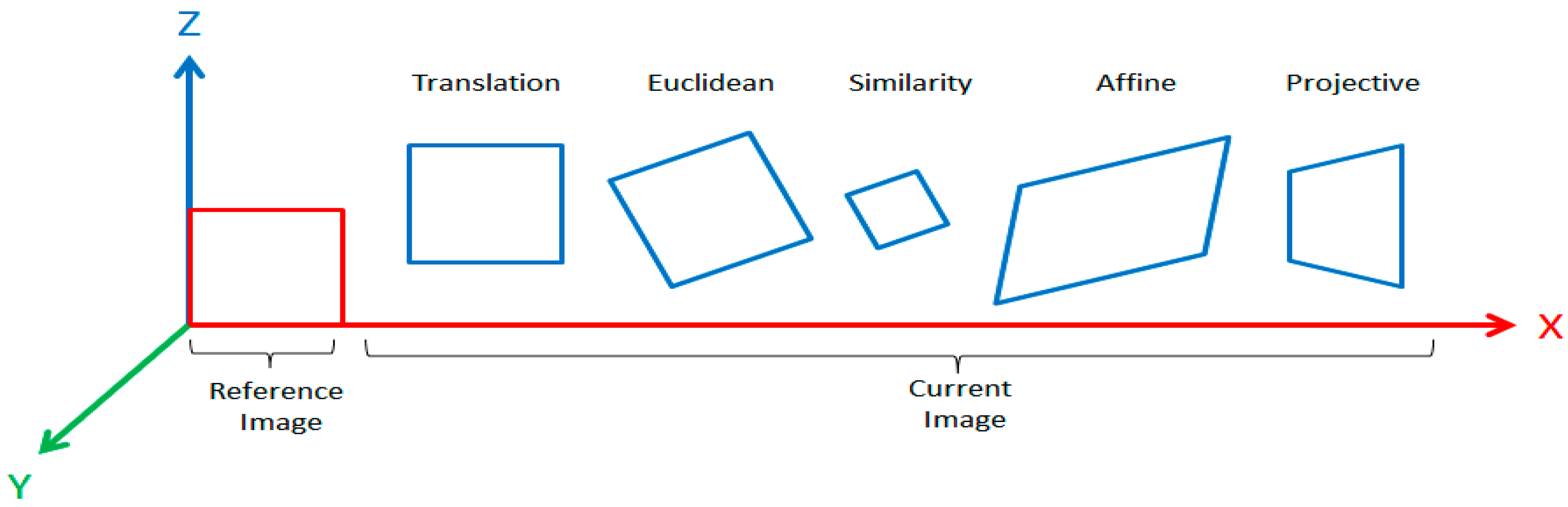
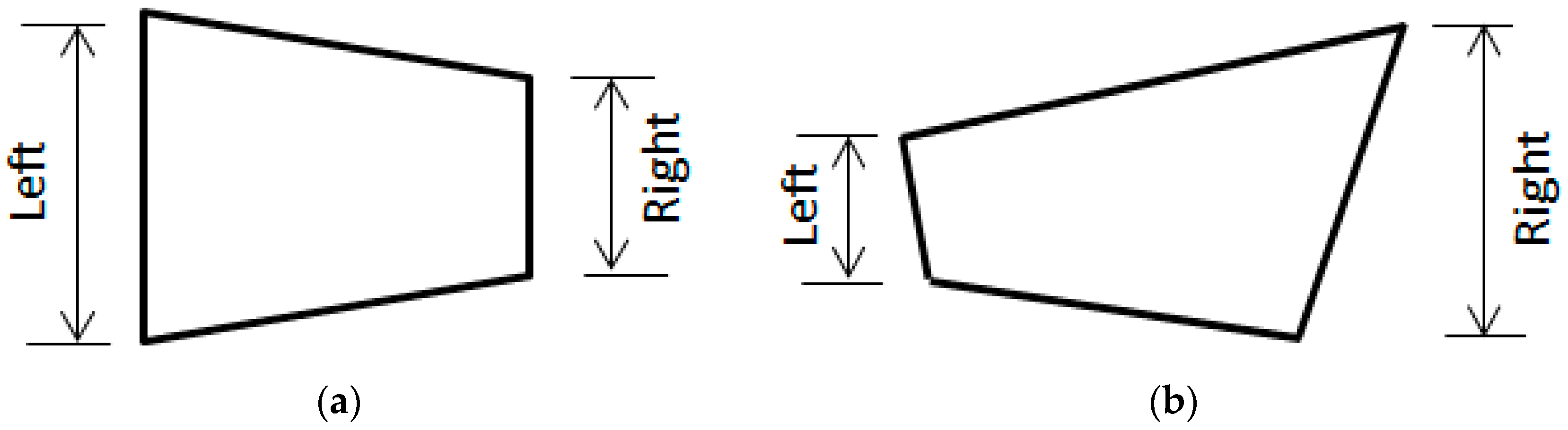
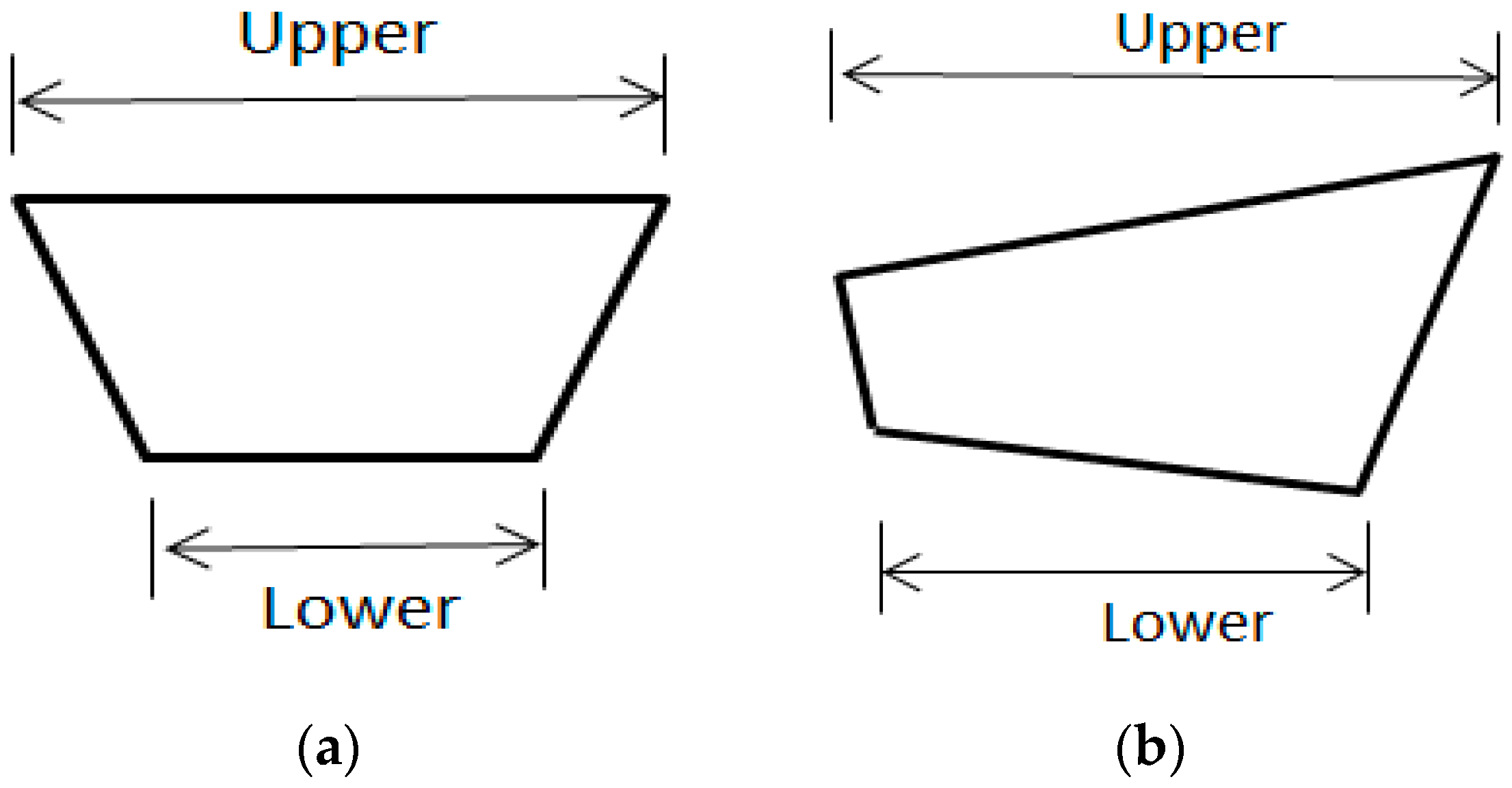
2.1. Image Transformation

According to Szeliski [1], the first step in matching two images is to detect or extract the distinct features of these images. However, this is not easy. Feature detection is challenging because when two images (e.g., the key reference frame and current frame) have been captured from a scene at different viewpoints, their features such as position, orientation, and scale are not exactly the same. This phenomenon is called image transformation. Thus, image transformation is impacted based on the position and orientation of the camera. The position and orientation of a camera depends on six spatial degrees of freedom, including three degrees of freedom for position (i.e., X, Y, and Z), and three degrees of freedom for orientation (i.e., pitch, roll, and yaw/head) [43]. Figure 6 illustrates the coordinate system that can be defined based on six degrees of freedom.

2.2. Image Transformation Scenarios: Illustrative Case Study (i.e., Examples of Image-Based Scene Transformations)

To have a better understanding of camera position and orientation and their impact on image transformation, an illustrative case study has been conducted. In this case study, a camera was installed on a tripod with six degrees of freedom. In this first step, a reference picture was captured from a scene with a fixed camera’s orientation and position. In the second step, the secondary pictures were captured from a different camera’s position and orientation. For each capture, only one degree of freedom was applied. In other words, three pictures were captured when the position of the camera changed in the X, Y, or Z directions with a fixed orientation, and three pictures were captured while the position was fixed and the orientation changed in the X, Y, or Z directions. The six images captured in these ways were aligned over the reference picture separately to identify the transformation impacts and based on the observations, six conceptual diagrams were created, as shown in Figure 7.
The first type is a linear transformation that occurs on the X-axis. This type occurs when the relative position of a camera changes in the X direction while producing two images. The second type is a linear transformation on the Z-axis. This transformation occurs when the camera is repositioned in the Z direction. The third type of linear transformation occurs on the Y-axis. In this type, which is correlated with scaling, the picture is captured when the position of the camera in the Y direction is changed. In this type, the size of objects in the image changes. The fourth type is an angular transformation that occurs around the X-axis. In this type, the orientation of the camera changes, and the camera is rotated around in the X direction. The fifth type is an angular transformation that occurs around the Y-axis. In this type, the camera rotates in the Y direction. The sixth type is an angular transformation that occurs on the Z-axis. In this type, the camera is rotated around in the Z direction.
In the first and second types of transformations, only the locations of objects in the images change. In the third type, in addition to the locations of objects, the sizes of the objects change. In the fourth type of transformation, the locations of objects change. In the fifth and sixth types of transformations, due to changes in the orientation of the camera, the shapes of objects in the image change. In addition to these changes, in all these transformations, due to changes in the position of the camera or changes in orientation, some objects that are captured on the first image disappear and some new objects are captured.

Advanced Transformations

In real situations, without using a tripod, these fundamental transformations combine and create new types of transformations. For instance, if transformations on the X- and Z-axis coincide, it is called translation. In this type, it is assumed that factors such as image orientation, lengths, angles, parallelism, and straight lines remain unchanged. In other words, this type of transformation only has two degrees of freedom. If relative translation and the rotation of the camera lens regarding the Y-axis occur together, it is called Euclidean (rigid). In this type, factors such as lengths of edges, angles, parallelism, and straight lines remain unchanged. In other words, this type of transformation has three degrees of freedom.
The third type, similarity, occurs when the relative rotation and scale of the second image changes in relation to the first image. This means that the second picture, in addition to the rotation of the camera around the Y-axis, was captured from a different position relative to the scene (on the Y-axis). In this type, angles, parallelism, and straight lines remain unchanged. In other words, this type of transformation has four degrees of freedom. The fourth type, called affine, occurs when a camera that takes the second picture rotates around two coordination axes such that parallelism and straight lines remain unchanged. In other words, this type of transformation has six degrees of freedom.
The fifth type, which is called projective (homography), occurs when a camera rotates around one or more coordination axes such that only the straight lines remain unchanged. In other words, this type of transformation has eight degrees of freedom.
The image matching algorithms need to deal with these image transformations and bring them into agreement with the reference picture. To have a better understanding, Szeliski [1] suggested a diagram to visualize these different types of transformations (Figure 8).

2.3. Propose an Approach Based on Localization Systems to Remotely Repeat and Retrieve the Camera’s Position and Orientation to Decrease Image Transformation (Sensor-Based Tracking Systems)

As was previously indicated, at temporary and messy places such as construction sites, one way to potentially decrease the impact of image transformation is a system that navigates the crews to hold the camera in a single position and orientation without using a tripod or a fixed-point camera. For this purpose, an accurate positioning and orientation system is required. Sensor-based techniques, independent from vision techniques, could be suitable candidates. In other words, sensor-based approaches use non-vision sensors to track a scene. Mechanical sensors, magnetic sensors, GPS (Global Positioning System), and ultrasonic and inertia sensors are some examples of non-vision tracking sensors. The following paragraph introduces the limitations of these types of sensors.
GPS has low user coverage in an indoor environment (4.5%) [45]. It requires direct lines of sight from a user’s receiver to at least three orbital satellites [46,47] and its signal accuracy is degraded by occlusion. Wi-Fi has high user coverage indoors (94.5%) [45], with 15 to 20 m accuracy in indoor environments [45]. Bluetooth has 75% accuracy for partial coverage and 98% accuracy for full coverage in a room, while target devices need to be stationary for long periods of time [48]. Ultrasonic sensors are sensitive to temperature, occlusion, and ambient noise, require significant infrastructure, and have a low update rate [47]. Infrared is short range and limited because of line-of-sight requirements, as seen in Active Badge [49]. Radio frequency (type of signals, IEEE 802.11, WLAN) has a median accuracy of 2 to 3 m [50]. Inertial sensors are prone to drift and require constant recalibration [51]. Radio frequency (type of signals, UWB) emits ultra-wideband signals that can pass through walls and have high accuracy [52,53].

Required Position and Orientation Sensors

From these different tracking sensors, the most accurate positioning system could be the system that works with ultra-wideband (UWB) [54]. The accuracy of this system claims to be (±)10 cm [54]. According to [54], “the accuracy achieved with this technology is several times better than traditional positioning systems based on WIFI, Bluetooth, RFID or GPS signals.” [54]. Some companies are developing UWB positioning sensors. One of them is called Pozyx. The sensors produced by this company include a tag and some anchors (at least four anchors are required). The tag sends and receives signals to anchor modules through a wireless radio technology called ultra-wideband (UWB) [54]. These signals can penetrate walls in an indoor environment. The anchor modules play the role of reference points for the tag. In this system, to calculate the position, the distance of one tag module to each anchor module is calculated based on time-of-flight (TOF) of the waves between the tag and anchors, where [54]:
  • Distance = time of flight × speed of light
  • Speed of light = 299,792,458 m/s
Then, through a method called multilateration [55], the position of the tag module with regard to anchor modules is calculated. For 3D orientation purposes, some sensors such as acceleration, magnetic field, and angular velocity are embedded in the tag module, which handles orientation responsibility. According to the sensor manual [54], each of these sensors has its own limitations, but through combining the outputs from different types of sensors, 3D orientation is computed accurately.

3. Methods

3.1. System Architecture: Positioning and Orientation

To better understand how these 3D positioning and orientation systems can be integrated and implemented for the purpose of this study, a system architecture was proposed. As shown in Figure 9, for the positioning estimations, the tag communicates with four anchors (i.e., reference points) through ultra-wideband RF signals. For orientation estimations, there are three sensors, acceleration, magnetic, and angular velocity, that can work together to estimate the tag orientation. The tag needs to be connected with a computing device such as a tablet to transfer the received data for analyzing and displaying to users. Using this information, the user can monitor the position and orientation of the tag. The first challenge is how can the tag be used for navigating the camera lens? The second challenge is how can data generated from the tag be displayed through a user interface for the purpose of monitoring the camera’s position and orientation? To meet these challenges, a prototype was developed.

3.2. Prototype Development

The prototype development included two phases. In the first phase, the positioning and orientation sensors were integrated with a tablet camera such that the sensors can detect any change in the position and orientation of the camera. In the second phase, a user interface was created to display information regarding the position and orientation of the camera so that users could monitor the position and orientation of the camera. The following paragraphs explain these phases in detail:
Phase 1 To use the tag module for navigating the camera’s lens, the simplest way could be attaching the tag module to the backside of the tablet in a fixed condition. To execute this idea, tape holders were used to attach the tag without any degrees of freedom. In this study, since the position and orientation of the tag relative to the tablet camera remained fixed, the position and orientation of the tag and camera lens were assumed to be the same. Figure 10 shows how the tag module was attached to the tablet.
Phase 2 To be able to display and monitor the positioning and orientation sensors outputs, a user interface was designed and prototyped (Figure 11). This user interface could collect the data regarding the position and orientation of the sensor tag and visualize that data in the form of dynamic diagrams simultaneously. The programming language Python was used to prototype this user interface, with Microsoft Windows selected as the operating system and Surface [56] selected as the handheld device to run this user interface. These systems were selected due to their compatibility with the sensors. Figure 11 illustrates the created user interface. The user interface included indicators that could display the position and orientation of the camera lens in the room. As shown in Figure 11, on the left side, two positioning indicators were designed. The first one could show the position of the tablet in the room on the X-Y axes. The second one could show the position of the tablet on the Z-axis.
On the right side, the orientation indicators are shown (Figure 11). The first one is related to the rotation of the tablet around the Z-axis, which is called the head. The second one is related to the rotation of the tablet around the Y-axis, which is called roll. The third one is related to the rotation of the tablet around the X-axis, which is called the pitch. The zero point on indicators occurred when the red point stopped at the center of the indicator. The fourth one is not an indicator. It was designed to illustrate the Cartesian coordinating system axes. This diagram was designed and displayed on the user interface next to indicators to make sure the participants were aware of the room’s coordination system during the experiment.
The user, by moving left and right, and forward and backward, could change the XY indicator; by moving up and down, the Z indicator; and by rotating the tablet, the pitch, roll, and head (i.e., yaw) indicators. After investigating the reference location and orientation, the user could look at the scene through the user interface screen and click the shutter button to capture a picture.

3.3. Experimental Testing of the Prototype System

To evaluate how the prototype approach (i.e., sensor-based approach) versus the traditional approach (i.e., non-sensor-based approach) could result in reducing image transformations in terms of accuracy and precision, an experiment was designed and conducted. The following sections explain the experiment design and the associated tasks.

3.3.1. Experimental Design

The experiment included two tasks. The first task was taking a picture from a scene without using positioning and orientation sensors, whereas the second task was taking a picture from the same scene but with the assistance of these sensors. The experiment was a within-subject experiment. In other words, each participant needed to conduct both tasks.
In this experiment, the pictures captured by participants were evaluated based on accuracy and precision parameters. Accuracy was defined as the capability of each approach to reproduce pictures that resemble a reference picture (i.e., error in accuracy = average transformations values − reference value). Our experimenter captured the reference picture from the scene before the experiment. The camera’s position and orientation to capture the reference picture were decided based on the common sense of the experimenter. In a real situation, this picture could be the first picture captured from a scene, and therefore other pictures need to be taken from the same viewpoint later. To measure errors regarding the accuracy of the captured images in contrast with the reference image, the average transformation values for each linear direction and angular orientation needed to be calculated separately. The results show how close the images are to the reference image.
In this experiment, precision was defined as the capability of each approach to reproduce pictures that resemble with each other (i.e., error in precision = standard deviation). To measure the error in precision, the standard deviation of transformation for each direction and angle needed to be calculated separately. The results show how close the transformation values are to one another.
For this experiment, a scene with unique features was selected (Figure 12). This scene was an image (172 × 120 cm) installed on a wall in a lab. This scene followed two criteria: (1) The design of the scene should not provide any measurement tool to the participants when they are conducting the experiment tasks. Measurements are only for data collection and analysis by the experimenter. For this purpose, instead of using a checkerboard that has straight lines and potentially could assist the participants in taking pictures and create bias in individual rating behavior, an image was used that looked like a broken window without any recognizable assists (e.g., straight lines) in its context. Although there was not any assist in the context of this image for participants, the design of this image was symmetrical. The experimenter could use this feature for data collection, measurements, and analysis purposes. (2) The image was installed inside a large room with an open zone. Therefore, the participants had enough space to conduct their tests without any physical barriers that could impact their behavior when capturing pictures.

3.3.2. Experiment Tasks

To conduct the experiment tasks, paper-based instructions were created and given to the participants before each task. These instructions included two separate parts. The first part explained the experiment process for the first task. To conduct the first task, each participant needed to read the first part of the instructions. Then, the participant received a tablet to take a picture from the scene. For the first task, the participants needed to use their common sense regarding the position and orientation of the tablet camera.
The second part of the instruction explained the process for the second task. To conduct the second task after completing the first task, the participants needed to read the second part of the instructions. Concurrently, the experimenter needed to equip the tablet with the sensor tag and run the associated python code to activate positioning so that orientation sensors could make the user interface indicators available to the participant. Thus, this time, the participant could monitor the position and orientation of the camera by viewing the indicators. Using these indicators, the participants needed to look for a reference viewpoint with the following features:
  • Position → XY = [0], Z = [0]
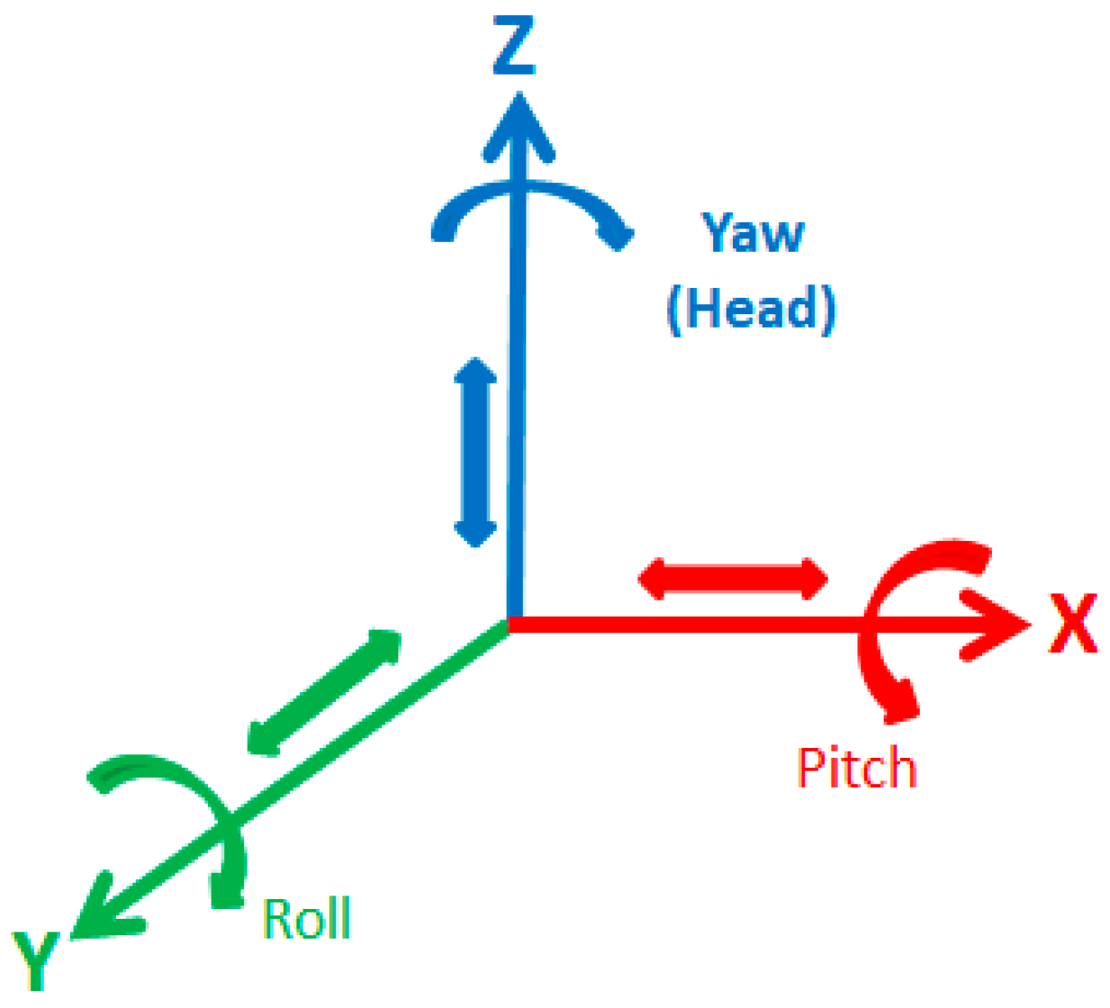
  • Orientation → Head = [0], Pitch = [0], Roll = [0].
To achieve the defined position, the participants could walk and change their position in different directions to find the reference position where XY = (0) and Z = (0). In addition, they could rotate the tablet around different directions to find the reference orientation where (pitch, roll, head) = (0, 0, 0). As was previously mentioned, this point of view (position and orientation) was defined based on the common sense of experimenter. For this reason, this point of view could not be predictable for participants. It was not located on a position at the center zone of the room or on an orientation angle perpendicular to the scene. It was the best image that the experimenter sensed could capture from the scene. During the second test, the experimenter monitored the participants to ensure they captured the pictures when the red points in all these indicators stopped on zero (0). For each task, the participants were allowed to generate only one picture. There were not any time limitations when participants read the guidelines and conducted the tasks for the experiment. Figure 13 illustrates the coordination system of the scene.

4. Results and Discussion

To conduct the experiment, 37 graduate and undergraduate students were randomly selected. For each task, 37 pictures were collected. The experiment was conducted at one location within similar indoor environment conditions and laboratory settings. The reference position and orientation value were similar for both tasks. To avoid learning effect, the first task was non-sensor-based for all the participants, because the second task, which involved the sensors, directed the participants to the defined reference position and orientation. The participants were tested individually to ensure they would not learn from each other. The pictures collected from the participants were divided into two groups (Appendix B). The first group included pictures related to the first task and the second group from the second task. The first group contained 37 pictures taken without using the sensor system, and the second group contained 37 pictures that were taken with assistance from the sensors.

4.1. Limitations

From 37 images in the second group, ten pictures were discarded due to systematic errors that the experimenter reported during the experiment. In addition, two pictures from the first group were discarded due to the extreme camera rotation (90 degrees) around the Z-axis. This skewed rotation changed the coordination system for two pictures, and therefore the results were not calculable. Furthermore, in this experiment, the indicator regarding the Z direction (positioning only) was decided to be off to increase the speed of the system. The initial tests showed that the average transformations in the Z direction were very similar to transformations in the X direction. Considering this point and due to technical limitations, the indicator related to Z was decided to be put in the “off” stetting during the experiment.
A tripod was used for the initial study to understand the relationship between the camera’s orientation and the ratios. The tripod was equipped with leveling and protractor tools. It was better if we used a digital one.
It could have been better if we used the original tablet sensors instead of the tag sensors to monitor the orientation. However, the main issue that we observed in both systems (tag and tablet sensors) needed recalibration. Any time that the orientation sensors were used, the yaw had a slight error. Therefore, we decided to use the tag that generated data for both position and orientation.
The UWB system is a promising method that can penetrate walls. However, this experiment was conducted inside an open area. Thus, the potential impact of barriers concrete walls, steel structures, and building infrastructure (e.g., stairs, furniture, machines, etc.) that could have block line-of-sight were not considered.
The intrinsic parameters of the camera for both tasks were the same. For both tasks, the same camera with the same zooming level was used. The participants could not change the zooming level. For extrinsic calibration, manual approaches were used, as are explained in the text. Minor errors could have be included, but since the same methods were implemented for both groups of pictures (i.e., sensor-based and non-sensor-based), the results were unbiased.
The scene included a flat image of 172 × 120 cm instead of a 3D object. The reason for this simplicity was reducing errors in calculations. This 2D scene could be enough to evaluate the precision and accuracy of the two approaches (sensor-based versus non-sensor-based) in retrieving the position and orientation of the camera.

4.2. Measuring Changes in Camera’s Position and Orientation

The features in two images can transfer (i.e., displace) if the position and orientation of the camera that captured those pictures change. In this research study, to understand what type of transformation results in a certain type of change in a camera’s position and orientation, some methods were determined. These methods could assist the authors in assessing the causes of image transformation in different pictures. These methods are described in the following paragraphs:
Change in the position of the camera in the Y direction To be able to measure any change in the position of the camera in the Y direction, the method illustrated in Figure 14 was used. In this method, the position of the scene is fixed, but the camera’s position changes. The distance between the current images in the scene can be estimated where (yy′= y × i/i′). In this equation, y is the distance between the scene to the camera that captured the reference picture, i is the distance between two points in the reference image, i′ is the distance between similar points in the current image, and y′ is the distance between the reference camera and the current one.
After estimating the distance of the camera to the scene for all pictures, to find the change in position of the camera, the average distances should be compared with the distance measured regarding the reference picture (i.e., accuracy) and also with each other (i.e., precision).
Change in the position of the camera in the X direction To measure the change in position of the camera in the X direction, a reference point was selected at the center of the board installed on the scene. The distance between this point and the center of the camera lens (i.e., the center of the picture) was measured for all pictures (Figure 15). Since the scales of the pictures were different, these distances were converted into a single scale to become comparable. To find the change in position of the camera, the average distances were compared with the distance measured in the reference picture (i.e., accuracy) and also with each other (i.e., precision).
Change in the orientation of the camera around the Y-axis (roll) To measure the orientation of the camera around the Y-axis, a horizontal line that crossed the center of image was drawn. Then, a protractor was used, and the angle that this line made with the image was measured as rotation around the Y-axis. To find the change in orientation of the camera around the Y-axis, the average rotations for each group were compared with the reference rotation (i.e., accuracy) and also with each other (i.e., precision).
Change in the orientation of the camera around the Z-axis (head) Since the images were two-dimensional, the rotation angle of the camera around the Z-axis was not easy to measure. Therefore, other variables were considered. These variables are the length of the left and right sides of an image that change when the rotation around the X-axis occurs. Turning the camera to the left expands the left side and reduces the right side, and vice versa (Figure 16). Knowing these principles, the left and right sides for all pictures from both groups were measured, and then the ratio for each one was measured (i.e., ratio = smaller vertical side/larger vertical side).
To understand the relationship between the camera’s orientation and these ratios, a separate test was conducted. In this test, a scene was provided, and a camera was installed on a tripod. The camera lens was leveled and located in a parallel position to the scene. The camera had only one degree of freedom around the Z-axis. In this condition, the first picture was captured. Next, the camera was rotated 10 degrees around the Z-axis, and the second picture was captured. This process was repeated, and the results were recorded. Using the results, a graph with a regression line was created (Figure 17). This graph was used to convert the image ratios related to the experimental data to meaningful rotation degrees.
To find the change in orientation of the camera around the Z-axis, the average rotation values of each group of pictures were compared with the reference rotation (i.e., accuracy) and also with each other (i.e., precision).
Change in the orientation of camera around the X-axis (pitch) To measure the orientation of the camera around the X-axis, the same principle and graph used for the Y-axis were applied for this axis. However, this time, turning the camera around the X-axis could impact the length of the upper and lower sides of the images. Therefore, the ratio for each image was measured (i.e., ratio = smaller horizontal side/larger horizontal side) (Figure 18).
To measure the degree of rotation around the X-axis, the graph illustrated in Figure 17 was used. To find the change in orientation of the camera around the X-axis, the average rotation values for each group of pictures were compared with the reference rotation (i.e., accuracy), and also with each other (i.e., precision).

4.3. Results of Camera’s Positioning Accuracy and Precision in the X and Y Directions

The results of the experiment to discuss the accuracy of the two approaches for producing pictures resembling the reference picture regarding the X and Y directions are presented in Table 1 and are explained as follows:
  • Accuracy in the X direction The results of the experiment regarding accuracy (i.e., producing pictures resembling the reference picture) showed that when the images were captured with the assistance of positioning sensors, they more accurately resembled the reference picture. In other words, when the participants did not use the sensors during the first task, the average error, in terms of accuracy in the X direction, was (30 cm), but when they used the sensors during the second task, the average error decreased to (0.3 cm).
  • Accuracy in the Y direction The same situation occurred in the Y direction. In the Y direction, which reflected scaling, the average accuracy error decreased from (33 cm) to (6.8 cm) when the participants used a positioning sensor during the second task.
So far, this sensor-based approach could produce more accurate results than the non-sensor-based approach by reducing image transformation in both X and Y directions. The results of the experiment to discuss the precision of two approaches in producing pictures resembling each other regarding the X and Y directions are explained as follows:
  • Precision in the X direction The results regarding precision (i.e., producing pictures resembling each other) in the X direction showed an exciting result. In this direction, precision decreased when the participants used the sensor-based approach. In other words, the pictures captured during the first task without sensors had less standard deviation (15.5 cm) as compared with those that were captured during the second task (21 cm). This result indicates that when the participants wanted to take pictures from the scene without sensors, based on their common sense, they selected locations in the X direction that better resembled the reference image (the X direction was parallel to the scene). Therefore, the degree of repeatability increased. In contrast, since the sensors inherently generated error, the participants were navigated to the locations in the X direction that were less close to each other. The results are shown in Table 1.
  • Precision in the Y direction The results of the experiment regarding precision determined when the images were captured with the assistance of positioning sensors showed that they were more precise in the Y direction. In other words, when participants used the sensors during the second task, the standard deviation in the Y direction decreased (from 112 cm to 13.3 cm). This result showed that in the Y direction, the positioning sensor during the second task could navigate the participants to distances that resembled the reference image more than the first task when they used their common sense.
Thus, in the Y direction, the standard deviation when participants used their common sense in selecting a location in the perpendicular direction to the scene (i.e., Y) was almost six times more than this value in the parallel direction with the scene (i.e., X). Furthermore, according to the sensor’s standard manual, the positioning sensor is expected to have errors between +10 and −10 cm. In this experiment, the average standard deviation of the positioning sensor was measured (21 cm) in the X direction and (13.3 cm) in the Y direction.
Another useful result that could be extracted from Table 1 is range (range = max − min). Subtracting the maximum from the minimum revealed that the maximum range occurred in the Y direction (582 − 154 = 505 cm) when the non-sensor-based approach was used. In contrast, the range value for the sensor-based approach was 366 − 312 = 54 cm. This result shows that in the worst-case scenario, the separation of data for the sensor-based approach is ten times better than that of the non-sensor-based approach. Regarding the X direction, when the sensor-based approach was used, the maximum range occurring in the X direction (101 − 11 = 90 cm) which was slightly more than when the non-sensor-based approach was used (77 − 0 = 77 cm).

4.4. Results of Camera’s Orientation, Accuracy, and Precision around the X, Y, and Z Directions

The results of the experiment to discuss the accuracy of two approaches in producing pictures resembling the reference image regarding the camera’s orientations around the X, Y, and Z axes are presented in Table 2 and are explained as follows:
  • Accuracy around the X-axis (pitch) The results of the experiment regarding accuracy (i.e., producing pictures resembling the reference picture) showed that the results in both approaches are very similar. While the orientation of the camera around the X-axis for the reference image was measured as 7 degrees, the average reference was 5 degrees for the first group of pictures and 2 degrees for the second group of pictures. Thus, the average accuracy error for pictures captured without using a sensor is slightly less (2 degrees vs. 5 degrees) than when the images were captured with the assistance of orientation sensors. This result shows that using the sensor did not improve the accuracy for rotation around the X-axis (pitch).
  • Accuracy around the Y-axis (roll) The results showed that the average accuracy around the Y-axis for both approaches is the same. While the orientation of the camera for the reference image around the Y-axis measured 0, the average orientation for Groups 1 and 2 (with and without sensors) measured the same (1 degree). This result showed that when participants wanted to take pictures from a scene using their common sense, they could hold the tablet camera almost in the same orientation as when they used the orientation sensors (Table 2). However, as was indicated in the limitation section, two of the pictures captured by participants had 90 degrees rotation around the Y-axis of the tablet. Although these two exceptional pictures were discarded because of the high statistical skews that could affect the calculations, this could occur in real situations if crews are not warned in advance.
  • Accuracy around the Z-axis (yaw) The results showed the average accuracy around the Z-axis for the sensor-based approach is slightly better than the non-sensor-based approach. While the orientation of the camera around the Z-axis for the reference image measured 10 degrees, the average for the non-sensor-based approach was 17 degrees and the sensor-based approach was 15 degrees. Therefore, the orientation accuracy error for the sensor-based approach (5 degrees) was slightly less than the non-sensor-based approach (7 degrees). This result indicates that the participants, using their common sense, can generate results closer to the reference than when they use sensors.
In general, the degree of resemblance of the pictures produced by both approaches is very close to the reference picture. The precision of the two approaches in producing pictures resembling each other regarding orientations around the X, Y, and Z axes is presented in Table 2 and explained as follows:
  • Precision around the X-axis (pitch) The result regarding the standard deviation for the sensor-based approach was less than the non-sensor-based approach (7 degrees vs. 2 degrees). Therefore, precision (i.e., producing pictures that resemble each other) around the X-axis improved when the participants used the sensor-based approach. While the precision error for the non-sensor-based approach was 7 degrees, this value decreased to 2 degrees when they used the sensor-based approach. Therefore, the degree of repeatability of the camera’s orientation and picture resemblance for pitch increased.
  • Precision around the Y-axis (roll) The standard deviation for both sensor-based and non-sensor-based approaches was almost the same (1.5 degrees vs. 1.2 degrees). Therefore, the results regarding the average precision error around the Y-axis (roll) were almost the same.
  • Precision around the Z-axis (yaw) The standard deviation around the Z-axis reduced from 20 degrees to 7 degrees when participants used the sensor-based approach. This means the precision error for the sensor-based approach is less, as the participants could repeat the orientation of the camera regarding (yaw) with less error when using the sensor-based approach.
The other interesting results presented in Table 2 could be the range values (range = max − min) of the changes in the camera’s position and orientation when the sample pictures were captured.
The maximum range in orientation occurred around Y (90 − 0 = 90 degrees) and Z (80 − 1 = 79 degrees) when the non-sensor-based approach was used. When the sensor-based approach was used, the maximum range in orientation occurred around Z (38 − 2 = 36 degrees). As was previously indicated, the SIFT algorithms cannot correctly identify the distinct points if the orientation is more than (30 degrees). Therefore, based on the results, the sensor-based approach can prevent this issue during the image capturing phase. Logically, the analysis of the captured images during the image matching phase by image matching algorithms is errorless.

5. Summary and Conclusions

Due to the wide use of image matching techniques in the construction industry, and the vulnerability of these techniques to correctly detect and match scene features when extreme transformations in images occur, this study aimed to investigate how to reduce image transformations. For this purpose, different scenarios in which image transformation can take place were visualized. It was shown how these transformations could occur when the position and orientation of a camera change in three linear directions and three angular orientations. As was illustrated, to reduce image transformations, changes in the viewpoint (i.e., position and orientation) of the camera needed to be reduced. For this purpose, different techniques were reviewed, and the most accurate one was selected. This technique included positioning sensors that worked based on UWB waves, and orientation sensors such as acceleration, magnetic, and angular velocity. To apply these sensors for the purpose of reducing image transformation, a system architecture was defined, and a prototype was developed. The development of the prototype included two phases. In the first phase, the positioning and orientation modules (i.e., tag and anchors) were integrated with a tablet camera such that these sensors could detect any change in the position and orientation of the camera. In the second phase, a user interface was created to display information regarding the position and orientation of the camera such that users could monitor the location and viewpoint of the camera.
To compare how using the sensor-based approach could be different than a non-sensor-based approach, in terms of decreasing changes in position and orientation of the camera, an experiment was designed and conducted. The experiment included two tasks. For the first task, the participants were asked to use their common sense to capture the best picture possible from a scene. For the second task, they were asked to capture a picture from the same scene but with the assistance of positioning and orientation sensors. The images participants generated for these two tasks were evaluated in terms of accuracy (i.e., producing pictures that resemble the reference picture), and precision (i.e., producing pictures that resemble each other). The results of the experiment demonstrated that when participants used the sensor-based approach, a significant reduction in accuracy errors in the X and Y directions, and also the precision error in the Y direction, was achieved. The precision error in the X direction was slightly higher when the participants used the sensor-based approach. Regarding the orientation, the average results for both approaches did not show a significant difference. While accuracy error was slightly better for the non-sensor-based approach for pitch, it was slightly worse for yaw, and the same for roll (however, if the two samples with 90 degree rotations were not discarded from data related to the non-sensor-based approach, the error for this approach increased significantly). For the sensor-based approach, precession errors were slightly lower for pitch and roll and moderately lower for yaw.
In conclusion, these results showed that applying the sensor-based approach can control the camera’s overall position and orientation and reduce image transformation. This can be important for feature detection algorithms used in applications such as augmented reality and change detections that use features of the environment in temporary and messy locations such as construction sites, where using a tripod or fixed-point camera is not possible. This research had technical limitations. The accuracy and precision of the sensor-based approach could improve. For instance, in this experiment, only four anchors were used. Using more anchors and even tags could improve the results. By using more powerful tablets, the time for data processing could be reduced, and the positioning system in the Z direction, which for this experiment was off, would be functioning. In future studies, the pictures produced by these two approaches could be tested by the image matching process to evaluate how the accuracy of the related algorithms could improve. If these limitations are eliminated by a sensor-based approach, failure scenarios such as extreme rotation and scaling, eliminated scene, and scene displacement can be improved.

Author Contributions

All authors contributed to the idea and concept of this study; Data curation, M.F.S. and J.L.; Formal analysis, M.F.S.; Funding acquisition, J.L.; Methodology, M.F.S. and J.L.; Project administration, J.L.; Software, M.F.S.; Supervision, M.G. and J.L.; Validation, M.G. and J.L.; Visualization, M.F.S.; Writing—original draft, M.F.S.; Writing—review & editing, M.G. and J.L. All authors have read and agreed to the published version of the manuscript.

Funding

This research was funded by the National Science Foundation (NSF), award number 1562515.

Conflicts of Interest

The authors declare no conflict of interest.

Appendix A

Augmented Reality: One technique that can link/combine paper-based and digital-based environments is augmented reality (AR). AR is “a technology that superimposes a computer-generated image (model) on a user’s view of the real world, thus providing a composite view” [58]. AR is a part of the reality–virtuality continuum [59] (Figure A1). According to Azuma [60], AR “allows the user to see the real world, with virtual objects superimposed upon or composited with the real world. Therefore, AR supplements reality, rather than completely replacing it.” In other words, AR is a combination of real-world and digital information through a single interface [21]. Thus, AR is an appropriate technology that can be used to access detailed information.
Figure A1. Concept of augmented reality [59].
Applsci 10 02305 g0a1
There are two types of AR techniques, i.e., marker-based and markerless. The following paragraphs explain the differences between these two techniques:
  • Marker-based AR (feature-based, artificial markers) In this approach, an artificial marker needs to be located in the scene or environment as a reference. Then, information about the marker is interpreted by a handheld computing device (smartphone/tablet) application. Artificial markers are printed and attached to the locations [1]. Some examples of artificial markers are dot-based markers [61], QR code markers [62,63], circular markers [64], square markers [65], and alphabetic combination markers [65]. Due to fiducial marker use in the environment, and the fact that these markers are distinguishable in the environment (physical world), the marker-based tracking approach is very robust with high accuracy [66,67,68].
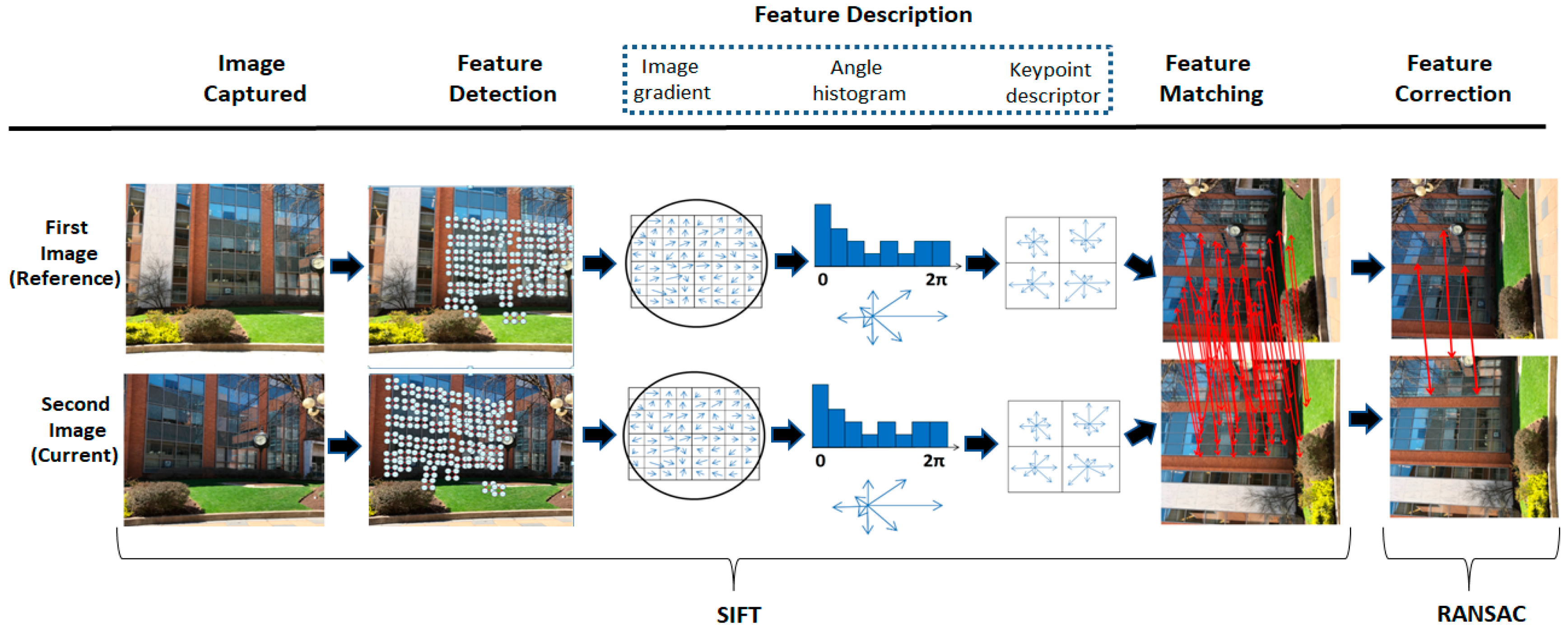
  • Markerless AR (feature-based, natural features) This type of AR system uses the natural features of the environment as references [24]. Depending on the algorithm used for this system, these features could be edges, corners, segments, or points [23]. In this online approach, features extracted from current video frames taken from the scene are compared with features extracted from an initial key frame. Then, correspondence between feature pairs is created. This loop continues until the best match between features has been computed [1]. If enough numbers of matches are identified, the virtual data stored in repository is queried and appears on the screen of the computing device, such as a smartphone or tablet.

Appendix B

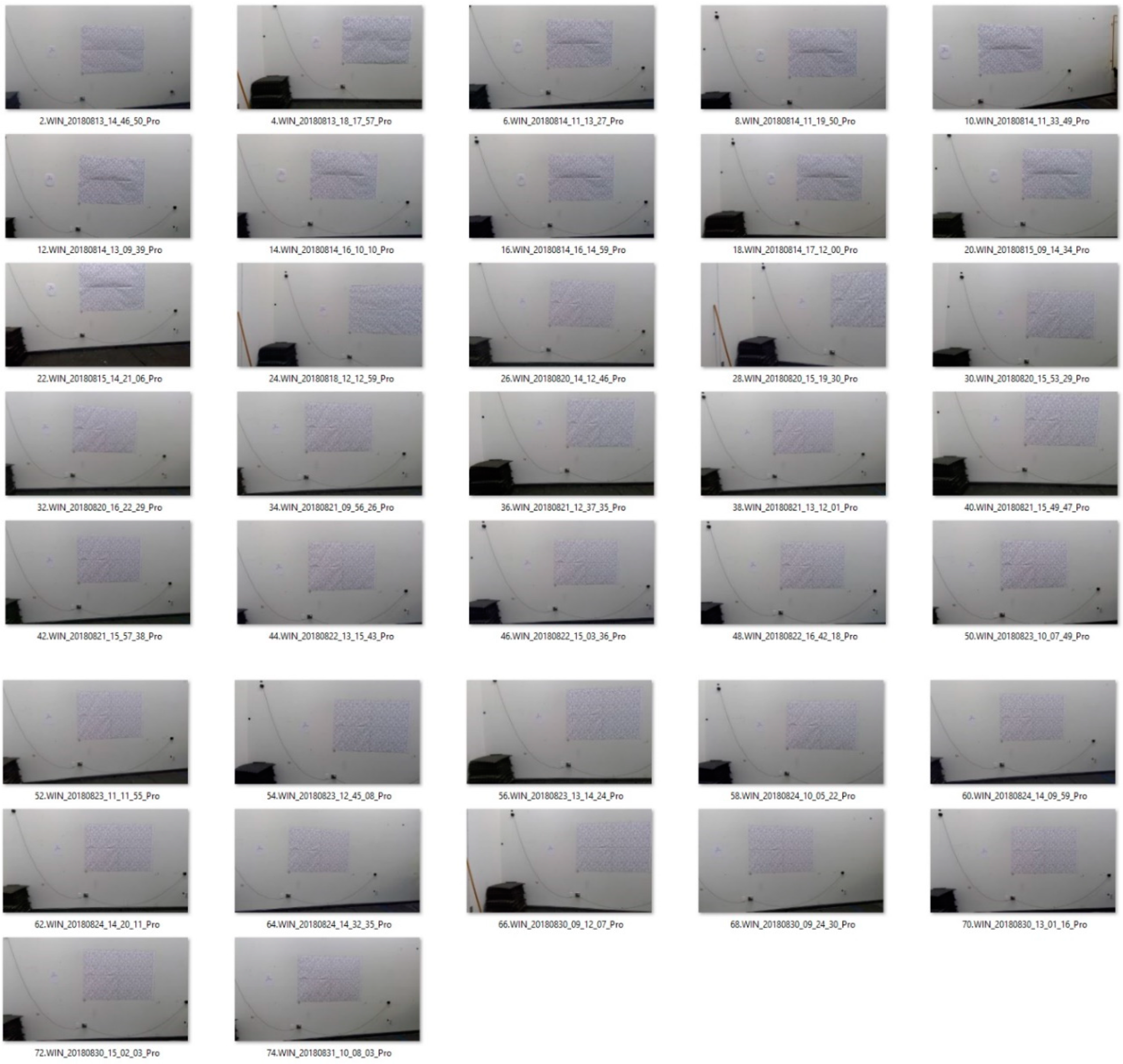
B.1. First Group of Samples

The first group of pictures was taken by 37 participants without using the positioning and orientation system during the first task. Figure A2 shows the collected data from the first task.
Figure A2. The first sample group of pictures.
Applsci 10 02305 g0a2

B.2. Second Group of Samples

The second group of pictures was taken by 37 participants using the positioning and orientation system during the second task. Figure A3 shows the collected data from the second task.
Figure A3. The second sample group of pictures.
Applsci 10 02305 g0a3

References

  1. Szeliski, R. Computer Vision: Algorithms and Applications. Computer (Long. Beach. Calif.) 2010, 5, 832. [Google Scholar]
  2. Forsyth, D.A.; Ponce, J. Computer Vision, A Modern Approach; Printice Hall: Upper Saddle River, NJ, USA, 2003. [Google Scholar]
  3. Shapiro, L.G.; Stockman, G.C. Computer Vision: Theory and Applications; Prentice Hall: Upper Saddle River, NJ, USA, 2001. [Google Scholar]
  4. Horn, B.; Klaus, B.; Horn, P. Robot Vision; MIT Press: Cambridge, NY, USA, 1986; ISBN 0262081598. [Google Scholar]
  5. Chen, M.; Shao, Z.; Li, D.; Liu, J. Invariant matching method for different viewpoint angle images. Appl. Opt. 2013, 52, 96–104. [Google Scholar] [CrossRef]
  6. Dai, X.L.; Lu, J. An object-based approach to automated image matching. In Proceedings of the IEEE 1999 International Geoscience and Remote Sensing Symposium. IGARSS’99 (Cat. No. 99CH36293), Hamburg, Germany, 28 June–2 July 1999; Volume 2, pp. 1189–1191. [Google Scholar]
  7. Karami, E.; Prasad, S.; Shehata, M. Image Matching Using SIFT, SURF, BRIEF and ORB: Performance Comparison for Distorted Images. In Proceedings of the 2015 Newfoundland Electrical and Computer Engineering Conference, St. John’s, NL, Canada, 14–15 April 2015; p. 4. [Google Scholar]
  8. Sinha, S.N.; Frahm, J.M.; Pollefeys, M.; Genc, Y. Feature tracking and matching in video using programmable graphics hardware. Mach. Vis. Appl. 2011, 22, 207–217. [Google Scholar] [CrossRef]
  9. Brown, M.; Lowe, D.G. Automatic panoramic image stitching using invariant features. Int. J. Comput. Vis. 2007, 74, 59–73. [Google Scholar] [CrossRef] [Green Version]
  10. Szeliski, R.; Shum, H.-Y. Creating full view panoramic image mosaics and environment maps. In Proceedings of the 24th Annual Conference on Computer Graphics and Interactive Techniques, Los Angeles, CA, USA, 3–8 August 1997; pp. 251–258. [Google Scholar]
  11. Kratochvil, B.E.; Dong, L.X.; Zhang, L.; Nelson, B.J. Image-based 3D reconstruction using helical nanobelts for localized rotations. J. Microsc. 2010, 237, 122–135. [Google Scholar] [CrossRef]
  12. Lu, Q.; Lee, S. Image-based technologies for constructing as-is building information models for existing buildings. J. Comput. Civ. Eng. 2017, 31, 4017005. [Google Scholar] [CrossRef]
  13. Moghaddam, B.; Pentland, A. Probabilistic visual learning for object representation. IEEE Trans. Pattern Anal. Mach. Intell. 1997, 19, 696–710. [Google Scholar] [CrossRef] [Green Version]
  14. Rowley, H.A.; Baluja, S.; Kanade, T. Neural network-based face detection. IEEE Trans. Pattern Anal. Mach. Intell. 1998, 20, 23–38. [Google Scholar] [CrossRef]
  15. Pérez-Lorenzo, J.; Vázquez-Martín, R.; Marfil, R.; Bandera, A.; Sandoval, F. Image Matching Based on Curvilinear Regions; IntechOpen: London, UK, 2007. [Google Scholar]
  16. Takacs, G.; Chandrasekhar, V.; Tsai, S.; Chen, D.; Grzeszczuk, R.; Girod, B. Rotation-invariant fast features for large-scale recognition and real-time tracking. Signal Process. Image Commun. 2013, 28, 334–344. [Google Scholar] [CrossRef]
  17. Tang, S.; Andriluka, M.; Schiele, B. Detection and tracking of occluded people. Int. J. Comput. Vis. 2014, 110, 58–69. [Google Scholar] [CrossRef]
  18. Kang, H.; Efros, A.A.; Hebert, M.; Kanade, T. Image matching in large scale indoor environment. In Proceedings of the 2009 IEEE Computer Society Conference on Computer Vision and Pattern Recognition Workshops, CVPR 2009, Miami, FL, USA, 20–25 June 2009; pp. 33–40. [Google Scholar]
  19. Kim, H.; Kano, N. Comparison of construction photograph and VR image in construction progress. Autom. Constr. 2008, 17, 137–143. [Google Scholar] [CrossRef]
  20. Jabari, S.; Zhang, Y. Building Change Detection Using Multi-Sensor and Multi-View- Angle Imagery; IOP Conference Series: Earth and Environmental Science; IOP Publishing: Halifax, NS, Canada, 2016; Volume 34. [Google Scholar]
  21. Gheisari, M.; Foroughi Sabzevar, M.; Chen, P.; Irizzary, J. Integrating BIM and Panorama to Create a Semi-Augmented-Reality Experience of a Construction Site. Int. J. Constr. Educ. Res. 2016, 12, 303–316. [Google Scholar] [CrossRef]
  22. Foroughi Sabzevar, M.; Gheisari, M.; Lo, L.J. Improving Access to Design Information of Paper-Based Floor Plans Using Augmented Reality. Int. J. Constr. Educ. Res. 2020, 1–21. [Google Scholar] [CrossRef]
  23. Belghit, H.; Zenati-Henda, N.; Bellabi, A.; Benbelkacem, S.; Belhocine, M. Tracking color marker using projective transformation for augmented reality application. In Proceedings of the 2012 International Conference on Multimedia Computing and Systems, Tangier, Morocco, 10–12 May 2012; pp. 372–377. [Google Scholar]
  24. Yuan, M.L.; Ong, S.-K.; Nee, A.Y.C. Registration using natural features for augmented reality systems. IEEE Trans. Vis. Comput. Graph. 2006, 12, 569–580. [Google Scholar] [CrossRef]
  25. Moravec, H.P. Techniques towards Automatic Visual Obstacle Avoidance. In Proceedings of the International Joint Conference on Artificial Intelligence, Cambridge, MA, USA, 22–25 August 1977; p. 584. [Google Scholar]
  26. Harris, C.G.; Stephens, M. A combined corner and edge detector. In Proceedings of the Alvey Vision Conference, Manchester, UK, 31 August–2 September 1988; pp. 147–151. [Google Scholar]
  27. Smith, S.M.; Brady, J.M. SUSAN—A new approach to low level image processing. Int. J. Comput. Vis. 1997, 23, 45–78. [Google Scholar] [CrossRef]
  28. Rosten, E.; Drummond, T. Fusing points and lines for high performance tracking. In Proceedings of the Tenth IEEE International Conference on Computer Vision (ICCV’05) Volume 1, Washington, DC, USA, 17–21 October 2005; Volume 2, pp. 1508–1515. [Google Scholar]
  29. Rosten, E.; Drummond, T. Machine learning for high-speed corner detection. In Proceedings of the European Conference on Computer Vision, Graz, Austria, 7–13 May 2006; pp. 430–443. [Google Scholar]
  30. Beaudet, P.R. Rotationally invariant image operators. In Proceedings of the 4th International Joint Conference on Pattern Recognition, Tokyo, Japan, 7–10 November 1978. [Google Scholar]
  31. Lakemond, R.; Sridharan, S.; Fookes, C. Hessian-based affine adaptation of salient local image features. J. Math. Imaging Vis. 2012, 44, 150–167. [Google Scholar] [CrossRef] [Green Version]
  32. Lindeberg, T. Scale selection properties of generalized scale-space interest point detectors. J. Math. Imaging Vis. 2013, 46, 177–210. [Google Scholar] [CrossRef] [Green Version]
  33. Lowe, D.G. Distinctive image features from scale-invariant keypoints. Int. J. Comput. Vis. 2004, 60, 91–110. [Google Scholar] [CrossRef]
  34. Mikolajczyk, K.; Schmid, C. Scale & affine invariant interest point detectors. Int. J. Comput. Vis. 2004, 60, 63–86. [Google Scholar]
  35. Bay, H.; Ess, A.; Tuytelaars, T.; Van Gool, L. Speeded-up robust features (SURF). Comput. Vis. Image Underst. 2008, 110, 346–359. [Google Scholar] [CrossRef]
  36. Yussof, W.N.J.H.W.; Hitam, M.S. Invariant Gabor-based interest points detector under geometric transformation. Digit. Signal Process. 2014, 25, 190–197. [Google Scholar] [CrossRef]
  37. Fischler, M.A.; Bolles, R.C. Random sample consensus: A paradigm for model fitting with applications to image analysis and automated cartography. Commun. ACM 1981, 24, 381–395. [Google Scholar] [CrossRef]
  38. Morel, J.-M.; Yu, G. ASIFT: A new framework for fully affine invariant image comparison. SIAM J. Imaging Sci. 2009, 2, 438–469. [Google Scholar] [CrossRef]
  39. Yu, G.; Morel, J.-M. A fully affine invariant image comparison method. In Proceedings of the 2009 IEEE International Conference on Acoustics, Speech and Signal Processing, Taipei, Taiwan, 19–24 April 2009; pp. 1597–1600. [Google Scholar]
  40. Yu, Y.; Huang, K.; Chen, W.; Tan, T. A novel algorithm for view and illumination invariant image matching. IEEE Trans. Image Process. 2011, 21, 229–240. [Google Scholar]
  41. Wu, J.; Cui, Z.; Sheng, V.S.; Zhao, P.; Su, D.; Gong, S. A comparative study of SIFT and its variants. Meas. Sci. Rev. 2013, 13, 122–131. [Google Scholar] [CrossRef] [Green Version]
  42. Dellinger, F.; Delon, J.; Gousseau, Y.; Michel, J.; Tupin, F. Change detection for high resolution satellite images, based on SIFT descriptors and an a contrario approach. In Proceedings of the 2014 IEEE Geoscience and Remote Sensing Symposium, Quebec City, QC, Canada, 13–18 July 2014; pp. 1281–1284. [Google Scholar]
  43. Höllerer, T.; Feiner, S. Mobile augmented reality. In Telegeoinformatics: Location-Based Computing and Services; Karimi, H.A., Hammad, A., Eds.; CRC Press: Boca Raton, FL, USA, 2004; ISBN 0-4153-6976-2. [Google Scholar]
  44. Sebastian Richard Hitting the Spot. Available online: http://spie.org/x26572.xml (accessed on 8 August 2019).
  45. LaMarca, A.; Chawathe, Y.; Consolvo, S.; Hightower, J.; Smith, I.; Scott, J.; Sohn, T.; Howard, J.; Hughes, J.; Potter, F. Place lab: Device positioning using radio beacons in the wild. In Proceedings of the International Conference on Pervasive Computing, Munich, Germany, 8–13 May 2005; pp. 116–133. [Google Scholar]
  46. Khoury, H.M.; Kamat, V.R. Evaluation of position tracking technologies for user localization in indoor construction environments. Autom. Constr. 2009, 18, 444–457. [Google Scholar] [CrossRef]
  47. Rolland, J.P.; Davis, L.D.; Baillot, Y. A survey of tracking technologies for virtual environments. In Fundamentals of Wearable Computers and Augmented Reality; CRC Press: Boca Raton, FL, USA, 2001; pp. 67–112. [Google Scholar]
  48. Bargh, M.S.; de Groote, R. Indoor localization based on response rate of bluetooth inquiries. In Proceedings of the First ACM International Workshop on Mobile Entity Localization and Tracking in GPS-Less Environments, San Francisco, CA, USA, 19 September 2008; pp. 49–54. [Google Scholar]
  49. Want, R.; Hopper, A.; Falcao, V.; Gibbons, J. The active badge location system. ACM Trans. Inf. Syst. 1997, 4, 42–47. [Google Scholar] [CrossRef]
  50. Bahl, P.; Padmanabhan, V.N. RADAR: An in-building RF-based user location and tracking system. In Proceedings of the Proceedings IEEE INFOCOM 2000. Conference on Computer Communications. Nineteenth Annual Joint Conference of the IEEE Computer and Communications Societies (Cat. No. 00CH37064), Tel Aviv, Israel, 26–30 March 2000; Volume 2, pp. 775–784. [Google Scholar]
  51. Karlekar, J.; Zhou, S.Z.Y.; Nakayama, Y.; Lu, W.; Chang Loh, Z.; Hii, D. Model-based localization and drift-free user tracking for outdoor augmented reality. In Proceedings of the 2010 IEEE International Conference on Multimedia and Expo, ICME 2010, Singapore, 19–23 July 2010; pp. 1178–1183. [Google Scholar]
  52. Deak, G.; Curran, K.; Condell, J. A survey of active and passive indoor localisation systems. Comput. Commun. 2012, 35, 1939–1954. [Google Scholar] [CrossRef]
  53. Gezici, S.; Tian, Z.; Giannakis, G.B.; Kobayashi, H.; Molisch, A.F.; Poor, H.V.; Sahinoglu, Z. Localization via ultra-wideband radios: A look at positioning aspects for future sensor networks. IEEE Signal Process. Mag. 2005, 22, 70–84. [Google Scholar] [CrossRef]
  54. Pozyx. Available online: https://www.pozyx.io/ (accessed on 8 August 2017).
  55. Popa, M.; Ansari, J.; Riihijarvi, J.; Mahonen, P. Combining cricket system and inertial navigation for indoor human tracking. In Proceedings of the 2008 IEEE Wireless Communications and Networking Conference, Las Vegas, NV, USA, 31 March–3 April 2008; pp. 3063–3068. [Google Scholar]
  56. Microsoft. Available online: https://www.microsoft.com/en-us/surface (accessed on 10 December 2017).
  57. Distance to Objects Using Single Vision Camera. Available online: https://www.youtube.com/watch?v=Z3KX0N56ZoA (accessed on 1 March 2020).
  58. Soanes, C. Oxford Dictionary of English; Oxford University Press: New York, NY, USA, 2003; ISBN 0198613474. [Google Scholar]
  59. Milgram, P.; Kishino, F. A taxonomy of mixed reality visual displays. IEICE Trans. Inf. Syst. 1994, 77, 1321–1329. [Google Scholar]
  60. Azuma, R.T. A survey of augmented reality. Presence Teleoperators Virtual Environ. 1997, 6, 355–385. [Google Scholar] [CrossRef]
  61. Bergamasco, F.; Albarelli, A.; Rodola, E.; Torsello, A. Rune-tag: A high accuracy fiducial marker with strong occlusion resilience. In Proceedings of the CVPR 2011, Providence, RI, USA, 20–25 June 2011; pp. 113–120. [Google Scholar]
  62. Kan, T.-W.; Teng, C.-H.; Chou, W.-S. Applying QR code in augmented reality applications. In Proceedings of the 8th International Conference on Virtual Reality Continuum and its Applications in Industry, Yokohama, Japan, 14–15 December 2009; pp. 253–257. [Google Scholar]
  63. Ruan, K.; Jeong, H. An augmented reality system using Qr code as marker in android smartphone. In Proceedings of the 2012 Spring Congress on Engineering and Technology, Xi’an, China, 27–30 May 2012; pp. 1–3. [Google Scholar]
  64. Naimark, L.; Foxlin, E. Circular data matrix fiducial system and robust image processing for a wearable vision-inertial self-tracker. In Proceedings of the Proceedings. International Symposium on Mixed and Augmented Reality, Darmstadt, Germany, 1 October 2002; pp. 27–36. [Google Scholar]
  65. Han, S.; Rhee, E.J.; Choi, J.; Park, J.-I. User-created marker based on character recognition for intuitive augmented reality interacion. In Proceedings of the 10th International Conference on Virtual Reality Continuum and Its Applications in Industry, Hong Kong, China, 11–12 December 2011; pp. 439–440. [Google Scholar]
  66. Pucihar, K.Č.; Coulton, P. Exploring the Evolution of Mobile Augmented Reality for Future Entertainment Systems. Comput. Entertain. 2015, 11, 1–16. [Google Scholar] [CrossRef] [Green Version]
  67. Tateno, K.; Kitahara, I.; Ohta, Y. A nested marker for augmented reality. In Proceedings of the 2007 IEEE Virtual Reality Conference, Charlotte, NC, USA, 10–14 March 2007; pp. 259–262. [Google Scholar]
  68. Yan, Y. Registration Issues in Augmented Reality; University of Birmingham: Edgbaston, Birmingham, UK, 2015. Available online: https://pdfs.semanticscholar.org/ded9/2aa404e29e9cc43a08958ca7363053972224.pdf (accessed on 1 February 2020).
Figure 1. While SIFT detects, describes, and matches the key points, RANSAC filters incorrect matches (Adapted from [1,33]).
Applsci 10 02305 g001
Figure 2. Differences between the reference and current images when the camera’s orientation and position change, which results in transformation of the features of the current images. (a) Reference frame; (b) Current frame impacted by rotation; (c) Current frame impacted by scaling.
Applsci 10 02305 g002
Figure 3. An example of a scene in which its features have completely changed during renovation. (a) Image captured before renovation (reference image); (b) Image captured after renovation (current image).
Applsci 10 02305 g003
Figure 4. An example of two scenes in one room during renovation. (a) West wall captured (before renovation); (b) North wall captured (after renovation).
Applsci 10 02305 g004
Figure 5. Holding a camera in a single position and orientation on a jobsite. (a) Using a fixed-point camera for each scene on a jobsite; (b) Embedding a benchmark (point of reference) for each scene on a jobsite.
Applsci 10 02305 g005
Figure 6. Coordinate system including six degrees of freedom, three linear and three angular (adapted from [44]).
Applsci 10 02305 g006
Figure 7. Changes in the camera’s position and orientation can cause image transformation.
Applsci 10 02305 g007
Figure 8. Two-dimensional (2D) geometric image transformations (adapted from Szeliski [1]).
Applsci 10 02305 g008
Figure 9. Positioning and orientation system architecture.
Applsci 10 02305 g009
Figure 10. Physical integration of tag and tablet to be used on jobsite.
Applsci 10 02305 g010
Figure 11. User interface prototype.
Applsci 10 02305 g011
Figure 12. The scene in which participants were asked to capture pictures.
Applsci 10 02305 g012
Figure 13. Cartesian coordination system of scene.
Applsci 10 02305 g013
Figure 14. The method used to calculate the camera distance to the scene (adapted from [57]).
Applsci 10 02305 g014
Figure 15. Distance between center of lens and center of the board installed on the wall.
Applsci 10 02305 g015
Figure 16. How to measure the length of vertical sides. (a) If the vertical sides are parallel; (b) If the vertical sides are not parallel.
Applsci 10 02305 g016
Figure 17. Relationship between the image sides’ ratios and the camera’s degree of rotation.
Applsci 10 02305 g017
Figure 18. How to measure the length of horizontal sides. (a) If horizontal sides are parallel; (b) If horizontal sides are not parallel.
Applsci 10 02305 g018
Table 1. Comparison between accuracy and precision of the two approaches regarding linear transformation.
Type of ImageThe Distance between the Center of Lens and Center of the Fixed Point on SceneIn the X Direction (cm)In the Y Direction (cm)In the Z Direction (cm)
Reference image 44.71330.5N/A
Group 1 (without sensor)Avg.14.7297N/A
Min.0154N/A
Max.77582N/A
Precision Error (SD)15.5112N/A
Accuracy Error3033N/A
Range77428N/A
Group 2 (with sensor)Avg.45337N/A
Min.11312N/A
Max.101366N/A
Precision Error (SD)2113.3N/A
Accuracy Error0.36.8N/A
Range9054N/A
Table 2. Comparison between accuracy and precision of sensor-based and non-sensor-based approaches regarding the camera’s orientation factors (i.e., pitch, roll, and yaw/head).
Type of ImageRotationPitch (Ratio), DegreeRoll DegreeYaw or Head (Ratio), Degree
Reference image (0.97), 70(0.96), 10
Group 1 (without sensor)Avg.(0.98), 51(0.93), 17
Min.(1), 00(1), 0
Max.(0.85), 386.5 [90 *](0.69), 80
Precision Error (SD)(0.03), 71.5(0.08), 20
Accuracy Error(0.01), 21(0.03), 7
Range386.5 [90 *]80
Group 2 (with sensor)Avg.(0.99), 21(0.94), 15
Min.(1), 00(0.99), 2
Max.(0.96), 104.5(0.85), 38
Precision Error (SD)(0.01), 21.2(0.03), 7
Accuracy Error(0.02), 51(0.02), 5
Range104.536
* Two of the pictures captured by participants had a 90 degrees rotation around the Y-axis of the tablet. Although these two exceptional pictures were discarded because of the high statistical skews that could impose on the affect calculations, this can occur again in real situations if the crews are not warned in advance.

