An Unsupervised Deep Learning System for Acoustic Scene Analysis

Abstract

Acoustic scene analysis has attracted a lot of attention recently. Existing methods are mostly supervised, which requires well-predefined acoustic scene categories and accurate labels. In practice, there exists a large amount of unlabeled audio data, but labeling large-scale data is not only costly but also time-consuming. Unsupervised acoustic scene analysis on the other hand does not require manual labeling but is known to have significantly lower performance and therefore has not been well explored. In this paper, a new unsupervised method based on deep auto-encoder networks and spectral clustering is proposed. It first extracts a bottleneck feature from the original acoustic feature of audio clips by an auto-encoder network, and then employs spectral clustering to further reduce the noise and unrelated information in the bottleneck feature. Finally, it conducts hierarchical clustering on the low-dimensional output of the spectral clustering. To fully utilize the spatial information of stereo audio, we further apply the binaural representation and conduct joint clustering on that. To the best of our knowledge, this is the first time that a binaural representation is being used in unsupervised learning. Experimental results show that the proposed method outperforms the state-of-the-art competing methods.

1. Introduction

Acoustic scene analysis, has received a lot of research attention recently [1,2], which aims to recognize acoustic environments [3,4]. It finds applications in many audio devices, such as cars, robots, context-aware mobile devices, and intelligent monitoring systems. Conventional acoustic scene analysis was mainly supervised, and was named acoustic scene classification. A challenge named detection and classification of acoustic scenes and events, which focuses on the acoustic scene classification, has been launched for several years as well. The supervised methods classify audio segments or frame-level features into predefined acoustic environments using a classifier, such as the support vector machine [5], Gaussian mixture model [6], or deep convolutional neural network [7,8].

With the rapid development of multimedia technologies, a large number of unlabeled, real-world audio data points are being collected everyday. Analyzing the unlabeled data effectively is an important and challenging problem. However, the effectiveness of supervised acoustic scene classification relies heavily on the quality of manually-labeled data. It is known that labeling large-scale unlabeled acoustic data manually for the classifier training is time-consuming and expensive. Moreover, manual labels cannot be always accurate, which brings new challenges into the model training procedure [9]. In addition, the semantic labeling of acoustic scenes is also challenging, since the predefined categories may contain a hierarchical structure, and a real-world acoustic scene may contain multiple labels or unclearly-defined scenarios [1]. Unsupervised learning provides a solution to the aforementioned problems, as it does not require predefined label set and manually-labeled training data. In unsupervised learning, clustering is the method to group a set of data so that data in the same cluster are more similar than to those in other groups. It is usually used to analyze the statistic characteristics of the data.

In recent years, few clustering methods have been developed [10,11]. However, unsupervised acoustic scene analysis has not been well studied yet. Traditional methods partition audio clips into a set of acoustic scenes by a clustering algorithm, such as spectral clustering [12], co-clustering [13], or hierarchical clustering [14]. Because the acoustic features of the audio are usually high dimensional, it is difficult to apply a clustering algorithm directly to large-scale audio data. To deal with this problem, it is necessary to first reduce the dimensions of the features by a dimensionality reduction method. For example, Li et al. first used sparse subspace clustering (SSC) with a random sketching method to reduce the dimensions of some features for a low computational cost, and then adopted an online low-rank subspace clustering (OLRSC)-based algorithm for the acoustic scene clustering [15]. They further improved the performance using a joint clustering algorithm, named joint OLRSC (JOLRSC) [9], which takes both the original feature and the feature in the low-rank subspace as the input of the clustering.

In this paper, we propose an unsupervised acoustic scene analysis algorithm based on auto-encoder networks, named joint auto-encoder network with spectral clustering (JAESC), for stereo audio clips. Specifically, JAESC first extracts a high-dimensional binaural representation containing spatial information from the stereo audio clips. Then, the auto-encoder network is used to extract a low dimensional bottleneck feature from a high-dimensional acoustic feature and large-scale data via a so-called bottleneck architecture. Finally, we conduct joint clustering for the final partition. The main contributions of our paper are summarized as follows:

• The auto-encoder network extracts bottleneck features in an unsupervised way for a compact audio representation;
• The binaural representation is applied to utilize the spatial information of stereo audio for the unsupervised acoustic scene analysis;
• A joint clustering algorithm with the binaural representation is proposed for multi-channel audio data.

The proposed method has been compared with the state-of-the-art methods [9,15]. Experimental results on the TUT Acoustic Scenes 2017 data show that the proposed method outperforms the other methods significantly.

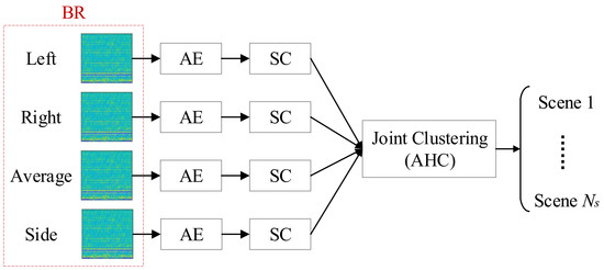
2. The Proposed Method

As shown in Figure 1, the proposed method includes three successive modules: a binaural representation (BR), an ensemble of auto-encoder networks (AEs), and a backend containing spectral clustering (SC) with agglomerative hierarchical clustering (AHC). Specifically, the binaural representation first expands each stereo audio clip into four channels named left, right, average, and side channels, and then extracts Mel-frequency cepstral coefficients (MFCC) from the four channels. Subsequently, four AEs are trained, each for a single channel. Four bottleneck features are extracted from the ensemble of AEs individually. These features are further transformed into four low-dimensional vectors by the Laplacian eigen-decomposition of SC. Finally, an AHC-based joint clustering with the four low-dimensional vectors is conducted. We present the method in detail as follows.

2.1. Binaural Representation

A stereo audio recording $\mathbf{s}$ consists of a left-channel recording ${\mathbf{s}}_l$ and a right-channel recording ${\mathbf{s}}_r$. It is believed that the two channels of a stereo audio recording have complementary information. Traditional approaches transform the stereo audio into monaural audio by simply averaging the signals of the two channels; i.e., ${\mathbf{s}}_a=({\mathbf{s}}_l+{\mathbf{s}}_r)/2$. This preprocessing decreases the signal-to-noise ratio, particularly in a situation in which the sound source or the microphone array is moving. To utilize the complementary information of the two channels of stereo audio, a binaural representation has been used in supervised acoustic scene classification [16]. Here, we apply it into unsupervised acoustic scene clustering.

The binaural representation contains four channels, which are the left channel ${\mathbf{s}}_l$, right channel ${\mathbf{s}}_r$, average channel ${\mathbf{s}}_a$, and side channel ${\mathbf{s}}_s$ respectively, where ${\mathbf{s}}_s={\mathbf{s}}_l-{\mathbf{s}}_r$ records the arrival time difference between the sound waves recorded by the two microphones. We denote the binaural representation as ${\mathbf{s}}_b=\{{\mathbf{s}}_l,{\mathbf{s}}_r,{\mathbf{s}}_a,{\mathbf{s}}_s\}$. Then, MFCCs are extracted from the four channels respectively, and we denote them as $\Omega$.

2.2. Auto-Encoder Network

An auto-encoder network is a powerful unsupervised dimensionality-reduction technique. Different from handcraft features, an auto-encoder network can learn an internal representation automatically by the optimization method. As illustrated in Figure 2, a deep auto-encoder network consists of two modules, an encoder and a decoder. The encoder $f_E$ produces a low-dimensional representation x from the high-dimensional input $\omega$; i.e., $x=f_E(\omega )$. Then the encoded vector x is fed to the decoder $f_D$ to reconstruct the original input $\omega$ as faithfully as possible; i.e., $\widehat{\omega }=f_D\left(x\right)$, where $\widehat{\omega }$ is an estimate of $\omega$ [17]. The network is trained by minimizing the loss $L(\omega ,\widehat{\omega })$ between $\omega$ and $\widehat{\omega }$. Thus, it does not need manual labels of training data during the network training. There is an overlap between the encoder and decoder, named the bottleneck, which is the narrowest hidden layer of the entire network. The output of the bottleneck is called the bottleneck feature, i.e., x, which used as a compact representation of $\omega$ [18].

Our auto-encoder network consists of five fully connected layers.

Table 1. Architecture of the deep auto-encoder network. Dense refers to fully connected layers. The numbers 576, 500, and 40 are the numbers of neurons. BN refers to batch normalization layer. Mish and sigmoid are activation functions.

Input: Original Features-576
Encoder	Dense-500-BN-Mish
	Dense-500-BN-Mish
	Dense-40-Sigmoid
Decoder	Dense-500-BN-Mish
	Dense-500-BN-Mish
	Dense-576
Output: Reconstructed features

shows the detailed architecture of the network. Specifically, we expand each input frame with adjacent frames by a contextual window and reduce the dimensionality of the input with a discrete cosine transform so as to avoid overfitting. Batch-normalization layers are added for the rapid and stable convergence of the network training. Mish [19] is used as the activation function which is represented as:

$$f\left(z\right)=ztanh(ln(1+e^z)).$$

(1)

This state-of-the-art activation function leads to a faster convergence rate and better performance than conventional activation functions. Note that the activation function at the bottleneck layer is still the sigmoid function, which is designed to produce a reasonable probability distribution.

We set the dimensions of both the input layer and output layer of the auto-encoder $N_I$ to 576. The neuron number of the bottleneck $N_B$ is set to 40, and the neuron numbers $N_H$ of all other hidden layers are set to 500 respectively. Finally, we average the 40-dimensional frame-level bottleneck features of each audio clip in dimensions for a segment-level feature x.

2.3. Spectral Clustering

Spectral clustering first learns a new representation of the input data points by conducting Laplacian eigen-decomposition to the affinity matrix of the data, and then conducts clustering on the new representation [20]. Differently from common clustering algorithms that operate in the original data space, spectral clustering focuses on the correlation between the data points in a kernel-induced feature space. Therefore, it leads to good clustering accuracy and robustness to noise. We present its usage in our system as follows.

Suppose that $x_n$ denotes the feature of the nth audio recording, and X denotes the set of the feature vectors for spectral clustering; i.e., $X=\{x_1,\dots ,x_N\}$, where N is the number of the audio recordings. In our system, we first use Gaussian kernel to construct an affinity matrix A:

$$A_{kl}=exp\left(-\frac{d{(x_k,x_l)}^2}{2\epsilon {\sigma }_k{\sigma }_l}\right),1\le k,l\le N,$$

(2)

where $d(x_k,x_l)$ is the Euclidean distance between $x_k$ and $x_l$; ${\sigma }_k$ and ${\sigma }_l$ are two scaling factors for the feature vectors $x_k$ and $x_l$ respectively; and $A_{kl}$ denotes an element of A at the kth row and lth column. The scaling factor ${\sigma }_k$ is defined in a nonparametric way:

$${\sigma }_k={\Sigma }_{x_l\in X_{l\ne k}}d(x_k,x_l)/(N-1),$$

(3)

which is the average distance between $x_k$ and all remaining points. $\epsilon$ is a tunable global scaling factor to control radial ranges. We searched $\epsilon$ through a set of values and found the system has the best performance when it is set to 20 in this work.

Subsequently, a standard procedure of spectral clustering is carried out. Specifically, we first create a normalized Laplacian matrix L, as follows:

$$L=D^{-1/2}A{D}^{1/2},$$

(4)

where D is a diagonal matrix in which $D_{ii}$ equals to the sum of all elements of the ith column of A. Decomposing the normalized Laplacian matrix L with eigenvalue decomposition produces the eigenvalues ${\left\{{\lambda }_n\right\}}_{n=1}^N$ and their corresponding eigenvectors ${\left\{{\nu }_n\right\}}_{n=1}^N$ of L. We choose the eigenvectors that correspond to the largest $N_c$ eigenvalues to form a matrix $V=[{\nu }_1,{\nu }_2,\dots ,{\nu }_{N_c}]\in R^{N\times N_c}$, where $N_c$ is the number of clusters. Then, we generate a matrix Y by renormalizing each row of V:

$$Y_{ij}=\frac{V_{ij}}{{\left({\Sigma }_j{V}_{ij}^2\right)}^{1/2}},1\le i\le N,1\le j\le N_c.$$

(5)

Finally, the jth row of Y is a new representation of the ith audio clip produced by spectral clustering, which is used as the input of the joint clustering.

2.4. Joint Clustering

Differently from the joint clustering proposed by Li et al. [9], which concatenates original acoustic features and their low-rank representations as the input of AHC for unsupervised acoustic scene clustering, here we adopt joint clustering with the binaural representation, which simply concatenates the four low-dimensional representations produced by the four spectral clustering as the input of AHC.

3. Experiments

3.1. Datasets

We conducted experiments on the TUT Acoustic Scenes 2017 dataset [21]. The dataset contains 4680 real-world stereo audio clips recorded from 15 different acoustic scenes, such as train, cafe/restaurant, office, home, forest path, lakeside beach, library, grocery store and so on. Each scene consists of 312 stereo audio recordings. Each recording is 10 seconds long and the sampling frequency of audio is $44.1$ kHz.

3.2. Comparison Methods and Parameter Setting

The proposed method was compared with the state-of-the-art JOLRSC method [9]. In the JOLRSC method, the MFCC feature was extracted and flattened, and then fed into the online low-rank subspace clustering (OLRSC). Specifically, both the original feature and the feature in the low-rank subspace are used for joint clustering.

To investigate the effects of the binaural representation and the auto-encoder-based monaural system on performance separately, we further studied the average-channel component of JASEC, named monaural auto-encoder network with spectral clustering (MAESC). MAESC first extracts MFCC from only average channel; then uses an auto-encoder network to extract a bottleneck feature; and finally adopts spectral clustering and AHC for clustering. We compared MAESC with SSC [15] and OLRSC [9], since all of them operate on the average channel of the stereo audio clips.

For a fair comparison, we adopted the same data preprocessing and feature extraction procedure as that in [9,15]. Specifically, the audio clips were resampled to 16 kHz. The frame length was set to 256 and the hop size was set to 160. We extracted 12-dimensional MFCCs and their one order and first and second difference coefficients, which formed 36-dimensional features.

3.3. Evaluation Criteria

We adopted clustering accuracy (ACC) and normalized mutual information (NMI) [22] as the evaluation criteria, which are two standard metrics for unsupervised clustering. ACC is the highest classification accuracy among all candidate classification accuracies produced from any possible permutation mappings, where the optimal permutation mapping is found by the Hungarian algorithm. NMI was proposed to overcome the permutation mapping problem between the ground-truth labels and the predicted labels. Note that NMI has a strong one-to-one association with classification accuracy. The detailed formula is shown in [22]. The higher the ACC and NMI scores are, the better the clustering quality is.

3.4. Main Results

Because the comparison of SSC, OLRSC, and JOLRSC methods in [9,15] used the TUT Acoustic Scenes 2017 dataset as well, we simply copied their results from them. The comparison results are presented in

Table 2. Performances of the other methods on the TUT Acoustic Scenes 2017 dataset.

Methods	SSC [15]	OLRSC [9]	MAESC (Ours)	JOLRSC [9]	JAESC (Ours)
ACC (%)	25.31	43.64	45.60	45.84	49.47

. Since only the performance on ACC were reported in [9,15], we report the ACC comparison results accordingly. From the Table 2, we observe that the proposed MAESC has a better performance than SSC and OLRSC, which manifests that the deep auto-encoder network is a more powerful dimensionality reduction method than the low-rank subspace method in OLRSC.

With joint clustering, we also observe that the proposed JAESC also outperforms the JOLRSC method, which proves that the proposed joint clustering scheme is also more efficient than that adopted by JOLRSC. Specifically, JOLRSC conducts joint clustering on the original feature and its low-rank subspace feature in subspace. Once the original feature of high dimensionality is used for clustering, computational cost will rapidly increase. On the contrary, the proposed JAESC conducts joint clustering on four low-dimensional features, which leads to a lower computational cost than JOLRSC.

As aforementioned, two channels of stereo audio have complementary information to some extent. It can be utilized by binaural representation and joint clustering. To further study the complementary information between the four channels of the binaural representation, we present the results of each channel in

Table 3. Performances of the different channels of stereo audio with the proposed methods. “Left”, “Right”, “Average”, and “Side” refer to four channels of binaural representation. “JAESC” refers to joint clustering with four channels.

	Left	Right	Average	Side	JAESC
ACC (%)	42.95	41.09	45.60	43.59	49.47
NMI (%)	45.13	46.00	48.01	45.40	53.20

. We can find that four channels of binaural representation yield different performances because they contain different information. The average channel (i.e., MAESC) leads to the best performance among the four channels. The results also show that jointly using all four channels leads to significantly better performance than using any of the four channels separately in terms of both ACC and NMI, which demonstrates that the four channels contain much complementary information. Moreover, the result also proves that a binaural representation can boost the performance of unsupervised tasks.

3.5. Effect of the Dimension of Bottleneck Feature

An auto-encoder network can compress the input feature into a low-dimensional vector, but also loses the information to some degree, which varies with the dimensions of the bottleneck feature. Therefore, we also study the dimensions of the bottleneck feature in Figure 3. From the figure, we see that the proposed system shows a stable performance on both evaluation metrics, when the dimensions of the bottleneck feature vary from 30 to 70. That shows promising practical usage.

4. Conclusions

In this paper, a joint auto-encoder network with a spectral clustering algorithm for unsupervised acoustic scene analysis is proposed. Specifically, the binaural representation is extracted from each audio clip first. Then, four low-dimensional vectors are extracted from the binaural representation using the deep auto-encoder network and spectral clustering. Subsequently, agglomerative hierarchical clustering is used for joint clustering on the low-dimensional vectors to boost the performance. From this study, we show that deep auto-encoder network is a good dimensionality reduction approach for unsupervised acoustic scene analysis, and it is more powerful and effective than the low-rank subspace methods. In addition, the complementary information between different channels of stereo audio is also very useful for unsupervised tasks. In future, we will further improve our system via two aspects: network architecture and clustering method. Since the audio are sequential data, recurrent neural networks will be introduced due to their capability of processing sequential data. Then, other clustering methods will be studied, such as Gaussian mixture variational autoencoders [10,11].

References

1. Barchiesi, D.; Giannoulis, D.; Stowell, D.; Plumbley, M.D. Acoustic scene classification: Classifying environments from the sounds they produce. IEEE Signal Process. Mag. 2015, 32, 16–34. [Google Scholar] [CrossRef]
2. Green, M.C.; Murphy, D. EigenScape: A Database of Spatial Acoustic Scene Recordings. Appl. Sci. 2017, 7, 1204. [Google Scholar] [CrossRef] [Green Version]
3. Ye, J.; Kobayashi, T.; Toyama, N.; Tsuda, H.; Murakawa, M. Acoustic Scene Classification Using Efficient Summary Statistics and Multiple Spectro-Temporal Descriptor Fusion. Appl. Sci. 2018, 8, 1263. [Google Scholar] [CrossRef] [Green Version]
4. Battaglino, D.; Lepauloux, L.; Pilati, L.; Evans, N. Acoustic context recognition using local binary pattern codebooks. In Proceedings of the 2015 IEEE Workshop on Applications of Signal Processing to Audio and Acoustics (WASPAA), New Paltz, NY, USA, 18–21 October 2015. [Google Scholar]
5. Rakotomamonjy, A.; Gasso, G. Histogram of gradients of time-frequency representations for audio scene classification. IEEE/ACM Trans. Audio Speech Lang. Process. 2015, 23, 142–153. [Google Scholar]
6. Park, S.; Mun, S.; Lee, Y.; Ko, H. Score Fusion of Classification Systems for Acoustic Scene Classification; Tech. Rep.; DCASE2016 Challenge: Budapest, Hungary, 2016. [Google Scholar]
7. Han, Y.; Park, J. Convolutional Neural Networks with Binaural Representations and Background Subtraction for Acoustic Scene Classification; Tech. Rep.; DCASE2017 Challenge: Munich, Germany, 2017. [Google Scholar]
8. Chen, H.; Liu, Z.; Liu, Z.; Zhang, P.; Yan, Y. Integrating the Data Augmentation Scheme with Various Classifiers for Acoustic Scene Modeling; Tech. Rep.; DCASE2019 Challenge: Tokyo, Japan, 2019. [Google Scholar]
9. Li, S.; Gu, Y.; Luo, Y.; Chambers, J.; Wang, W. Enhanced streaming based subspace clustering applied to acoustic scene data clustering. In Proceedings of the 2019 IEEE International Conference on Acoustics, Speech and Signal Processing (ICASSP), Brighton, UK, 12–17 May 2019. [Google Scholar]
10. Misra, D.; Dilokthanakul, N.; Mediano, P.; Garnelo, M.; Lee, M.; Salimbeni, H.; Arulkumaran, K.; Shanahan, M. Deep unsupervised clustering with Gaussian mixture variational autoencoders. arXiv 2016, arXiv:1611.02648. [Google Scholar]
11. Smieja, M.; Wolczyk, M.; Tabor, J.; Geiger, B. SeGMA: Semi-Supervised Gaussian Mixture Auto-Encoder. arXiv 2019, arXiv:1906.09333v1. [Google Scholar]
12. Xue, J.; Wichern, G.; Thornburg, H.; Spanias, A. Fast query by example of environmental sounds via robust and efficient cluster-based indexing. In Proceedings of the 2008 IEEE International Conference on Acoustics, Speech and Signal Processing (ICASSP), Las Vegas, NV, USA, 31 March–4 April 2008. [Google Scholar]
13. Cai, R.; Lu, L.; Hanjalic, A. Co-clustering for auditory scene categorization. IEEE Trans. Multimed. 2008, 10, 596–606. [Google Scholar] [CrossRef] [Green Version]
14. Rychtrikov, M.; Vermeir, G. Acoustical categorization of urban public places by clustering method. In Proceedings of the International Conference on Acoustics NAG/DAGA, Rotterdam, The Netherlands, 23–26 March 2009. [Google Scholar]
15. Li, S.; Wang, W. Randomly sketched sparse subspace clustering for acoustic scene clustering. In Proceedings of the 2018 26th European Signal Processing Conference (EUSIPCO), Rome, Italy, 3–7 September 2018. [Google Scholar]
16. Eghbal, H.; Lehner, B.; Widmer, G. A hybrid approach with multi-channel i-vectors and convolutional neural networks for acoustic scene classification. In Proceedings of the 2017 25th European Signal Processing Conference (EUSIPCO), Kos, Greece, 28 August–2 September 2017. [Google Scholar]
17. Hinton, G.E.; Salakhutdinov, R.R. Reducing the dimensionality of data with neural networks. Science 2006, 313, 504–507. [Google Scholar] [CrossRef] [PubMed] [Green Version]
18. Yu, D.; Seltzer, M.L. Improved bottleneck features using pretrained deep neural networks. In Proceedings of the INTERSPEECH-2011, Florence, Italy, 27–31 August 2011. [Google Scholar]
19. Misra, D. Mish: A self regularized non-monotonic neural activation function. arXiv 2019, arXiv:1908.08681. [Google Scholar]
20. Ng, A.; Jordan, I.M.; Weiss, Y. On spectral clustering: Analysis and an algorithm. In Advances in Neural Information Processing Systems; Dietterich, T.G., Becker, S., Ghahramani, Z., Eds.; MIT Press: Cambridge, MA, USA, 2002; pp. 849–856. [Google Scholar]
21. Mesaros, A.; Heittola, T.; Virtanen, T. TUT database for acoustic scene classification and sound event detection. In Proceedings of the 24th European Signal Processing Conference (EUSIPCO), Budapest, Hungary, 29 August–2 September 2016. [Google Scholar]
22. Strehl, A.; Ghosh, J. Cluster ensembles—A knowledge reuse framework for combining multiple partitions. J. Mach. Learn. Res. 2003, 3, 583–617. [Google Scholar]
Figure 1. Block diagram of the proposed system, where the term “BR” refers to binaural representation, “AE” refers to an auto-encoder, “SC” refers to spectral clustering, “AHC” is short for agglomerative hierarchical clustering, and N s is the number of acoustic scenes for clustering.
Applsci 10 02076 g001
Figure 2. Block diagram of the auto-encoder network.
Applsci 10 02076 g002
Figure 3. The effect of the dimensions N B of the bottleneck features produced by MAESC on the average channel on performance in terms of ACC and NMI.
Applsci 10 02076 g003