Article

Coupling Elephant Herding with Ordinal Optimization for Solving the Stochastic Inequality Constrained Optimization Problems

by
Shih-Cheng Horng
1,* and
Shieh-Shing Lin
2
1
Department of Computer Science and Information Engineering, Chaoyang University of Technology, Taichung 413310, Taiwan
2
Department of Electrical Engineering, St. John’s University, New Taipei City 251303, Taiwan
*
Author to whom correspondence should be addressed.
Appl. Sci. 2020, 10(6), 2075; https://doi.org/10.3390/app10062075
Submission received: 17 January 2020 / Revised: 11 March 2020 / Accepted: 13 March 2020 / Published: 19 March 2020
(This article belongs to the Collection Bio-inspired Computation and Applications)

Abstract

:
The stochastic inequality constrained optimization problems (SICOPs) consider the problems of optimizing an objective function involving stochastic inequality constraints. The SICOPs belong to a category of NP-hard problems in terms of computational complexity. The ordinal optimization (OO) method offers an efficient framework for solving NP-hard problems. Even though the OO method is helpful to solve NP-hard problems, the stochastic inequality constraints will drastically reduce the efficiency and competitiveness. In this paper, a heuristic method coupling elephant herding optimization (EHO) with ordinal optimization (OO), abbreviated as EHOO, is presented to solve the SICOPs with large solution space. The EHOO approach has three parts, which are metamodel construction, diversification and intensification. First, the regularized minimal-energy tensor-product splines is adopted as a metamodel to approximately evaluate fitness of a solution. Next, an improved elephant herding optimization is developed to find N significant solutions from the entire solution space. Finally, an accelerated optimal computing budget allocation is utilized to select a superb solution from the N significant solutions. The EHOO approach is tested on a one-period multi-skill call center for minimizing the staffing cost, which is formulated as a SICOP. Simulation results obtained by the EHOO are compared with three optimization methods. Experimental results demonstrate that the EHOO approach obtains a superb solution of higher quality as well as a higher computational efficiency than three optimization methods.

Graphical Abstract

1. Introduction

The stochastic inequality constrained optimization problems (SICOPs) consider the problems of optimizing an objective function with respect to some variables in the presence of stochastic inequality constraints on those variables. The object value of SICOPs is evaluated using simulations, which is a way of modeling of a complex system in the real-world [1]. The target of SICOPs is to search for the optimal settings of a complex system whose objective function that needs to be optimized subject to the stochastic inequality constraints. The SICOPs belong to a category of NP-hard problems [2], which are a type of optimization problem for which most likely no polynomial algorithm can be devised. Furthermore, the large solution space causes the SICOPs to be more difficult to determine the optimal settings by traditional optimization methods within a reasonable time.
Various approaches are utilized to resolve the SICOPs, such as the stochastic gradient descent (stochastic approximation) methods [3], metaheuristic methods [4] and bio-inspired artificial intelligence [5]. However, the convergence of the stochastic gradient descent methods generally requires complicated assumptions on the cost function and the constraint set [3]. The metaheuristic approaches [4], such as the simulated annealing, tabu search and evolutionary algorithms (EA) [6], are adopted to search for the global optimum. Nevertheless, the metaheuristic approaches are highly dependent on the control parameters involved and require massively parallel implementations to yield results within an acceptable time. Bio-inspired artificial intelligence [5] discusses the collective behavior emerging within self-organizing societies of agents. Some instances of novel swarm intelligence (SI) approaches are: Brain storm optimization, whale optimization algorithm, sooty tern optimization, fireworks algorithm and elephant herding optimization (EHO) [7,8]. Despite the success of applying these SI techniques [9], several limitations and barriers have been identified [10].
To reduce the computing time of SICOPs, a heuristic method coupling elephant herding optimization (EHO) with ordinal optimization (OO) [11], abbreviated as EHOO, is presented to find a superb solution in an acceptable time frame. The EHOO method consists essentially of three parts, which are metamodel construction, diversification and intensification. First, a metamodel based on the regularized minimal-energy tensor-product splines (RMTS) [12] is adopted to approximately evaluate fitness of a solution. Next, we proceed with an improved elephant herding optimization (IEHO) to determine N significant solutions from entire solution space. Finally, an accelerated optimal computing budget allocation (AOCBA) is utilized to choose a superb solution from the N significant solutions. These three parts significantly reduce the computational effort required to solve SICOPs. Subsequently, the problem of staffing optimization in a one-period multi-skill call center is formulated as a SICOP that contains a large solution space. Finally, the EHOO method is employed to solve the problem of staffing optimization in a one-period multi-skill call center. The goal of staffing optimization in a one-period multi-skill call center is to decide an optimal number of agents for minimizing the operating cost while satisfying the service level constraints.
There are three contributions of this work. The first one is to develop an EHOO method to find a superb solution in an acceptable time for a SICOP which is lack of structural information. Both of IEHO and AOCBA are novel approaches to improve the performance of the original EHO and OCBA, respectively. The proposed IEHO has a faster convergence rate than the original EHO. The AOCBA saves more computing effort than the typical OCBA. The second one is to formulate the problem of the staffing optimization in a one-period multi-skill call center as a SICOP. The third one is to apply the EHOO method for solving the SICOPs in the staffing optimization of a one-period multi-skill call center.
The rest of the paper is organized as follows. Section 2 describes the mathematical formulation of SICOPs. Section 3 contains the solution method to find a superb solution of SICOPs. Section 4 introduces the staffing optimization in a one-period multi-skill call center, which is formulated as a SICOP. Then, the proposed solution method is employed to solve this SICOP. Section 5 discusses the simulation results and compares with three optimization approaches. Finally, Section 6 makes a conclusion.

2. Stochastic Inequality Constrained Optimization Problems

2.1. Mathematical Formulation

A typical SICOP can be stated formally as shown below [1].
min f ( x )
subject to
E [ g j ( x ) ] b j ,   j = 1 , , J
V x U
where x = [ x 1 , , x K ] is a K-dimensional solution vector, f ( x ) denotes the objective function, b j is a service level, E [ g j ( x ) ] is the expected value of the jth constrained function, J is the number of constraints, V = [ V 1 , , V K ] is the lower bound of a solution vector, and U = [ U 1 , , U K ] denotes the upper bound of a solution vector. Sufficient simulation replications should be carried out to assure a precise estimate of E [ g j ( x ) ] . Let L denote the number of simulation replications and g j ( x ) represent the measure of the th simulation replication. A straightforward approach to estimate E [ g j ( x ) ] is the sample mean that is computed as follows.
g ¯ j ( x ) = 1 L = 1 L g j ( x )
When the value of L increases, g ¯ j ( x ) obtains a better estimate of E [ g j ( x ) ] . There are two important issues that have been concerned in efficiency of stochastic simulation optimization. (i) L must be large if a sound estimate of E [ g j ( x ) ] is required, which has a decisive influence on the optimum that an optimization technique can find. (ii) g ¯ j ( x ) must be evaluated for various solutions to determine the best solution.
Since the stochastic inequality constraints are soft, the constrained problem (1)–(2) can be converted to an unconstrained one by addition of a quadratic penalty function [13].
min   F ( x ) = η × f ( x ) + ( 1 η ) × j = 1 J P F j ( x )
where η ( 0 , 1 ) denotes an integrated factor, F ( x ) represents an integrated objective function, and P F j ( x ) is a steep penalty function. The integrated objective function of (5) comprises two terms, the objective function (1) and the violated constraint functions in (2).
P F j ( x ) = { 0 , i f   g ¯ j ( x ) b j ( g ¯ j ( x ) b j ) 2 × 10 4 , e l s e
The penalty function is developed with a steep jump to ensure that the sample mean satisfies the service level. Since the objective function is penalized by addition of a penalty function, a large value of amplification 10 4 for violated service level constraints is to guarantee an obvious discontinuity of the quadratic penalty function. Let L a indicate the large value of L , and the accurate evaluation of (4) is referred to as L = L a . An accurate evaluation is defined as an evaluation that is tolerant of a small noise and modeling error. For simplicity, let F a ( x ) represent the integrated objective value of a x using accurate evaluation.
As pointed out by the OO method [11], order of a solution is likely kept even it is evaluated using a metamodel. To choose N significant solutions from solution space within an acceptable computation time, we should construct a metamodel to approximate the integrated objective function of a solution more rapidly and adopt an efficient search method assisted by this metamodel. The metamodel is based on the RMTSs [12], and the search method is the IEHO.

2.2. Difficulty of the Problem

Solving the SICOPs is more difficult because of (i) time-consuming fitness evaluation, (ii) a large solution space, and (iii) satisfaction of all stochastic inequality constraints. To resolve issues (i) to (iii) simultaneously, the OO method [11] is an attempt to circumvent these difficulties at least for the initial parts of optimization search. OO is adopted to supplement existing search approaches, but is not itself a search method. OO method can greatly reduce the computational complexity by emphasizing order rather than value while acquiring a good enough solution at a very high probability. The OO method has three basic steps. Firstly, a sampling subset is created by using a crude estimate to assess all solutions. A crude estimate provides a computationally fast evaluation of the performance for each solution. OO method specifies that order of solutions can be preserved even when evaluating by a crude estimate [11]. Secondly, a promising subset is selected from the sampling subset. Finally, candidate solutions in the promising subset are assessed using a precise estimate. A precise estimate can provide an accurate evaluation of a solution’s performance. The candidate solution with the optimal performance in the promising subset is the required good enough solution. There are already several successful applications of OO method to solve the expensive computing optimization problems, such as flow line production system [14], pull-type production system [15], and assemble-to-order systems [16].
OO method has emerged as an effective approach to simulation and optimization, but the stochastic inequality constraints dramatically reduce the computational efficiency in the SICOPs. Due to the tight computing budget, optimality in the SICOPs is usually traded off by a superb solution that can be obtained in real-time. In fact, using limited computing time to solve for a superb solution of SICOPs is the goal of this work. The key idea is to narrow the solution space stage by stage or gradually restrict the search range through iterative use of the OO method. The goal softening in the OO method is to relax the optimization goal from searching the best solution to seeking for a superb solution with high probability, which can ease the computational burden of finding the optimum. However, when the solution space is huge, the brute force evaluation using a crude estimate in the conventional OO method is not acceptable. To overcome this drawback, we need to use metamodels to ease the computational burden in the search process. Additionally, to explore more of the large solution space, a moderate population size should be kept in the optimization approach. According to the OO method, a metamodel is effective in separating good solutions from the bad. Therefore, we can use a metamodel-assisted optimization approach to find a small set of significant solutions from a large ranged solution space. In addition, if a precise estimate is applied to evaluate all the candidate solutions, it will be computational time-consuming. Therefore, to enhance efficiency, we can use a refined selection technique to replace the use of precise estimate for evaluating each candidate solution in the promising subset.

3. Solution Method

The solution method comprises of three parts, which are metamodel construction, diversification and intensification. The metamodel construction builds an RMTS metamodel to identify a set of likely solutions, the size of which can be a fraction of the size of the population. In the diversification part, the IEHO assisted by an off-line trained RMTS is utilized to search for N significant solutions within the large solution space. It has been shown in [12] that RMTS is competent in modeling complicated, nonlinear input–output relationships of discrete event simulated systems. In the intensification part, the AOCBA technique is used to identify the best solution among the N significant solutions found in diversification part. The AOCBA is aimed at obtaining an effective allocation rule such that the probability of correctly selecting the best alternative from a finite number of solutions can be maximized under a limited computing budget constraint.

3.1. Metamodel Construction

Various techniques are available to approximate the relationships between the inputs and outputs of a system. The purpose of metamodels is to approximate the predictions of the underlying model as accurately as possible and to be interpretable at the same time. There have been a various number of studies concerning distinct metamodels for particular applications, such as support vector regression [17], multivariate adaptive regression splines [18], kriging [19], artificial neural network [20], and RMTS [15]. Among them, RMTS adopts minimal energy and regularization to improve accuracy for low-dimensional problems with large unstructured datasets. Energy minimization has been used for specific applications such as extending a curve or surface with additional points. In RMTS, an energy function is treated as a cost minimization to determine the coefficients of the multivariate spline. RMTS has been successfully applied to curve fitting, function approximation, prediction, forecasting and classification [15]. The advantages of RMTS include fast prediction time, unsusceptible to training failure and scalability to the variability in parameters. Thus, a metamodel based on the RMTS is utilized to quickly estimate the fitness of a solution. The output variable of RMTS may be represented by a linear combination of a set of basis functions, where the coefficients are precomputed during training.
The training data patterns are ( x i , F a ( x i ) ), i = 1 , , M , where x i and F a ( x i ) denote the solution vector and objective value assessed using accurate evaluation, respectively. M represents the number of training data patterns, which can be determined from the sample size formula with a finite population correction factor. The framework of RMTS is displayed in Figure 1 [21] and the general model of RMTS can be stated formally as below.
f ( x | ω ) = i = 1 P ω i ψ i ( x )
where P denotes the number of basis functions, x denotes an input vector, ω = [ ω 1 , , ω P ] T is the vector of spline coefficients, ω i represents the coefficient of the multivariate spline, which provides a connection between the predicted f ( x | ω ) and basis functions ψ i ( ) . Two types of splines are commonly used as the basis functions: B-splines and cubic Hermite splines. The B-splines function is expressed as
ψ ( x ) = Q T B d ( x )
where Q is a vector of n coefficients and B d ( x ) is a vector of n B-spline piecewise functions. The piecewise functions in B d ( x ) are dth degree polynomial pieces in the variable x . Typically, third- or fourth-order degrees are used. The purpose of RMTS is to make each of its outputs f ( x | ω ) much closer to the actual expected values F a ( x ) .
RMTS solves an energy minimization function where the splines pass through the training points to obtain the coefficients ω i of the splines. The energy minimization function (9) comprises three terms, the second derivatives of the splines, regularization and approximation error related to the training points [21].
min ω 1 2 ( ω T H ω + δ ω T ω + 1 ξ i = 1 P ( ψ ( x i ) ω F a ( x i ) ) 2 )
where x i denotes the solution vector for the ith training data pattern, F a ( x i ) represents the output value of x i , H is the matrix containing the second derivatives, ψ ( x i ) = [ ψ 1 ( x i ) , , ψ P ( x i ) ] is the vector mapping the spline coefficients to the ith training output, ω is the vector of spline coefficients, δ is the weight of the term penalizing the norm of the spline coefficients, and ξ is the weight on gradient training data.
To reduce the on-line computation, the RMTS is trained off-line. After off-line training the RMTS, the output of f ( x | ω ) is computed by simple arithmetic operations for any x .

3.2. Diversification

With the aid of the RMTS metamodel, the conventional EHO can be used to select N significant solutions from the solution space. Since the EHO recursively improves the individuals in the elephant population, it is more suited to meet the needs. EHO is a biological algorithm inspired by the herding behavior of an elephant herd [7]. EHO is designed for solving and optimizing the optimizations problems by considering two herding behaviors, clan updating and separating. Clan updating operator is used to update the current positions of elephants and matriarch in each clan. Separating operator is used to upgrade the population diversity in the search process. There are many advantages of EHO, such as ease of implementation, simple control parameters and easy combination with other algorithms. EHO has been successfully employed to solve the human emotion recognition problems [22], energy-based localization problems [23] and multi-objective energy resource accommodation problem for distribution systems [24].
However, there are some issues of the original EHO, such as the low ability to retain the diversity during the search process and the cause of prematurity. Accordingly, the IEHO have been developed to improve the convergence efficiency of the original EHO. The IEHO has two control parameters that determine the influence of the matriarch and clans, which are scale factor for matriarch and scale factor for clans. The global exploration and exploitation of the IEHO are primarily dominated by the scale factor for matriarch. The IEHO adopts a large scale factor for the matriarch to increase diversification. When the scale factor for the matriarch is increased, the IEHO trends to perform global search while the probability of local search is decreased. In contrast, the IEHO utilizes a small scale factor for matriarch to increase intensification. When the scale factor for matriarch is decreased, the IEHO trends to perform local search around the optimum in a local region. The scale factor for clans defines the influence of the position for the elite elephant in a clan. Low value will generate new positions far from the center of a clan which induces a high level of exploration. Thus, a low value of scale factor for clans trends to global search, while a large value guides to local search.
The following notations are used in the IEHO. I is the number of clans, c i is the number of elephants in the ith clan, Φ = i = 1 I c i denotes the total number of elephants, t max is the number of required iterations. The position of the jth elephant in the ith clan at iteration t is denoted by x j i ( t ) = [ x j , 1 i ( t ) , , x j , K i ( t ) ] . The position of matriarch in the ith clan at iteration t is denoted by x b i i ( t ) = [ x b i , 1 i ( t ) , , x b i , K i ( t ) ] . α t is a scale factor that determines the influence of matriarch at iteration t, α t [ α min , α max ] , where α min and α max express the minimum and maximum values, respectively. β t is a scale factor that determines the influence of clans at iteration t, β t [ β min , β max ] , where β min and β max denote the minimum and maximum values, respectively.
IEHO (Algorithm 1) can be briefly summarized below.
Algorithm 1: The IEHO
Step 1: Configure parameters
Configure the values of I, K, c i , α min , α max , β min , β max , t max , and set t = 0 , where t expresses the iteration counter.
Step 2: Initialize clan
(a) A population of I clans is initialized with positions x j i ( 0 ) .
  For i = 1 , , I ,   do
  For j = 1 , , c i ,   do
   For k = 1 , , K ,   do
x j , k i ( 0 ) = V k + r a n d [ 0 , 1 ] × ( U k V k + 1 )

 where r a n d [ 0 , 1 ] denotes a random value generated in the range between 0 and 1, U k and V k
 denote the upper bound and lower bound of the solution variable, respectively.
(b) Calculate the fitness F ( x j i ( 0 ) ) of each elephant assisted by RMTS, i = 1 , , I , ,   j = 1 , , c i .
Step 3: Ranking
  Rank the c i individuals in the ith clan based on their fitness from low to high, then determine
  the elite elephant b i and the worst elephant w i in the ith clan.
Step 4: Clan updating
  Generate positions of the elite elephant b i by (12), and the others by (11).
  For i = 1 , , I , do
   For j = 1 , , c i , do
   For k = 1 , , K , do
    If j b i
x j , k i ( t + 1 ) = x j , k i ( t ) + α t × ( x b i , k i ( t ) x j , k i ( t ) ) × r a n d [ 0 , 1 ]

    Else
x b i , k i ( t + 1 ) = β t × 1 c i × j = 1 c i x j , k i ( t )

   r a n d [ 0 , 1 ] is a random value generated in the range between 0 and 1. If x j , k i ( t + 1 ) < V k , set
   x j , k i ( t + 1 ) = V k , and if x j , k i ( t + 1 ) > U k , set x j , k i ( t + 1 ) = U k .
Step 5: Separating
    Generate positions of the worst elephant w i .
    For i = 1 , , I , do
     For k = 1 , , K , do
x w i , k i ( t + 1 ) = V k + r a n d [ 0 , 1 ] × ( U k V k + 1 )

Step 6: Update scale factors
α t + 1 = α min + ( α max α min ) × exp ( ln ( α min α max ) 2 × t + 1 t max )
β t + 1 = β min + ( β max β min ) × ( 1 exp ( β max β min × t + 1 t max ) )

Step 7: Elitism
(a)
Calculate the fitness F ( x j i ( t + 1 ) ) assisted by RMTS. Rank the c i individuals in the ith clan based on their fitness from low to high, then determine the worst elephant x w i i ( t + 1 ) .
(b)
Replace the worst elephant x w i i ( t + 1 ) with the elite elephant x b i i ( t ) .

Step 8: Termination
  If t = t max , stop; else, set t = t + 1 and go to Step 3.
The IEHO stops when the maximum number of iterations, t max , has been reached. When the IEHO has terminated, the final Φ individuals are sorted based on their fitness. Then, the top N individuals are chosen as a candidate subset containing significant solutions.

3.3. Intensification

To enhance efficiency, an AOCBA method is developed as a more refined selection technique to identify the best solution among the significant solutions found in diversification part. In the original OCBA, it is necessary to perform all simulation replications repeatedly to calculate the statistics of overall simulation replications. The AOCBA requires only a part of extra simulation replications to determine the statistics of overall simulation replications. We proceed to determine a superb solution by the AOCBA approach from the N significant solutions. The AOCBA approach is designed to adjust the computational efforts dynamically for significant solutions. The key feature of the AOCBA is spending more computing resource on few remarkable solutions and less on most mediocre solutions. Focusing on few promising solutions does not only save computational time, but also reduces these promising estimators’ variances.
Through the statistics concerning objective value provided by the N significant solutions, the number of extra simulation replications is computed to provide more computational resource for promising solutions. Let C b denote the permissible computing budget, and L i indicate the number of simulation replications assigned to the i th solution. The initial number of simulation replications assigned to the N significant solutions is L 0 . The extra computing budget is raised by a pre-defined Δ at each iteration. The goal of the AOCBA is to properly allocate C b to L 1 , L 2 , …, L N such that L 1 + L 2 + + L N = C b and maximize the probability of obtaining the optimum. The permissible computing budget C b is obtained from C b = N × L a s , where L a = 104 indicates the simulation replications adopted in accurate evaluation and s is a time saving factor with respect to N that can be found in the optimal computing budget allocation (OCBA) procedure [25].
The step-wise process of the AOCBA (Algorithm 2) method is given below.
Algorithm 2: The AOCBA
Step 0. Set the quantity of L 0 , l = 0 , L 1 l = L 0 ,…, L N l = L 0 , where l expresses the iteration counter. Determine the value of C b = N × L a s .
Step 1: If i = 1 N L i l C b , stop and choose the optimum x * with the smallest objective value; else, go to Step 2.
Step 2: Raise an extra computing budget ( Δ ) to i = 1 N L i l , and update the simulation replications by
L j l + 1 = ( i = 1 N L i l + Δ ) × θ j l / ( θ b l + i = 1 , i b N θ i l )
L b l + 1 = θ b l θ j l × L j l + 1
L i l + 1 = θ i l θ j l × L j l + 1
for all i j b , where θ i l θ j l = ( δ i l × ( F ¯ b l F ¯ j l ) δ j l × ( F ¯ b l F ¯ i l ) ) 2 , θ b l = δ b l i = 1 , i b N ( θ i l δ i l ) 2 , F ¯ i l = 1 L i l h = 1 L i l F h ( x i ) , δ i l = 1 L i l h = 1 L i l ( F h ( x i ) F ¯ i l ) 2 , x i denotes the i th promising solution, F h ( x i ) is the objective value of x i for the h th simulation replication, and b = arg   min i F ¯ i l .
Step 3: Execute extra simulation replications (i.e., max [ 0 , L i l + 1 L i l ] ) for the i th promising solution, then calculate the mean ( F ^ i l + 1 ) and standard deviation ( δ ^ i l + 1 ) of these extra simulation replications using
F ^ i l + 1 = 1 ( L i l + 1 L i l ) h = L i l + 1 L i l + 1 F h ( x i )
δ ^ i l + 1 = 1 ( L i l + 1 L i l ) h = L i l + 1 L i l + 1 ( F h ( x i ) F ^ i l + 1 ) 2

Step 4: Update the mean ( F ¯ i l + 1 ) and standard deviation ( δ i l + 1 ) of overall simulation replications for the i th promising solution using
F ¯ i l + 1 = 1 L i l + 1 ( L i l × F ¯ i l + ( L i l + 1 L i l ) × F ^ i l + 1 )
δ i l + 1 = 1 ( L i l + 1 1 ) × ( L i l ( F ¯ i l ) 2 + ( L i l 1 ) ( δ i l ) 2 + ( L i l + 1 L i l ) ( F ^ i l + 1 ) 2 + ( L i l + 1 L i l 1 ) ( δ ^ i l + 1 ) 2 L i l + 1 ( F ^ i l + 1 ) 2 )
Let l = l + 1 and go to Step 1.

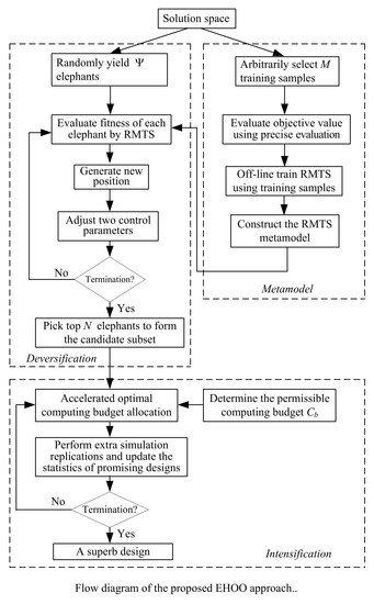
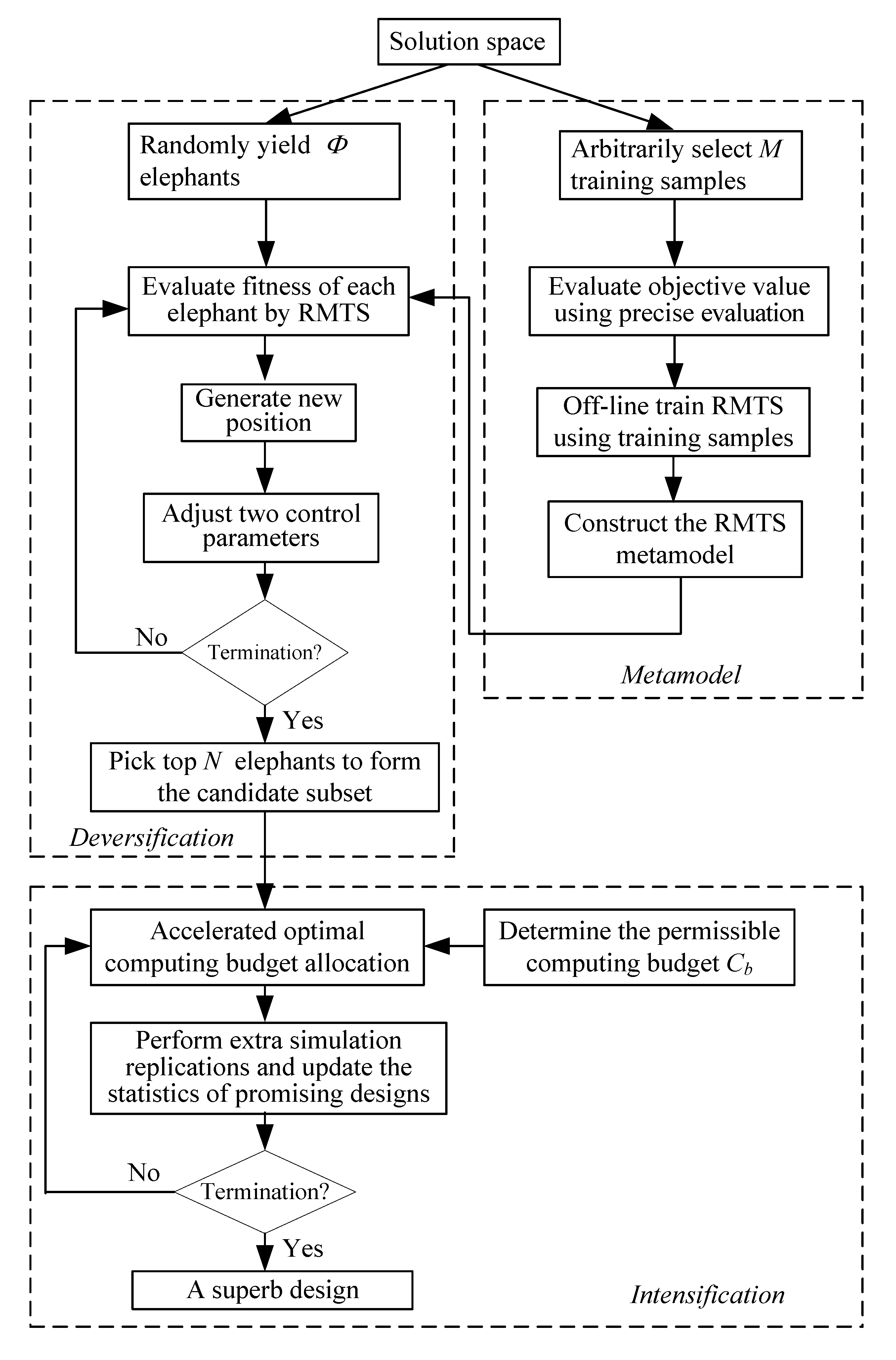
3.4. The EHOO Approach

Figure 2 presents the flow diagram of the EHOO approach (Algorithm 3). The step-wise procedure of the proposed EHOO is explained below.
Algorithm 3: The EHOO
Step 0: Configure the parameters of M , I, K, c i , α min , α max , β min , β max , t max , N , L a , L 0
  and Δ .
Step 1: Arbitrarily select M x’s from the solution space and evaluate F a ( x ) , then off-line train
  the RMTS using these M training samples.
Step 2: Arbitrarily choose Φ x ’s as the initial population and apply Algorithm 1 to these
  individuals assisted by RMTS. After Algorithm 1 terminates, rank all the final Φ x ’s based
  on their approximate fitness from low to high and choose the prior N x ’s to be the N
  significant solutions.
Step 3: Employ Algorithm 2 to the N significant solutions and find the optimum x * , and this
   one is the superb solution that we seek.

4. Application to Staffing Optimization of a Multi-Skill Call Center

4.1. A One-Period Multi-Skill Call Center

Call centers experience a growing proportion of the world economy. A call center is a centralized office used for delivering a large volume of enquiries by telephone, e-mail, chat and text [26,27]. Call centers offer very labor-intensive tasks, employing over millions of people around the world. Call centers play an important role in managing communications in several fields such as the banks, care hotlines, insurance companies, telemarketing, information centers, help-desks and emergency centers. Call centers usually handle various types of calls discriminated by the necessary skills to deliver a service. However, it is impossible or cost effective to train all agents to handle every type of call. Each agent group has a specified number of skills. In a multi-skill call center, agents can handle different call-types multiple types of calls. The types of calls are classified based on the type of service requested, such as the spoken language and the perceived value of customers. Agents in a multi-skill call center may not be able to handle all the different types of calls that are served by the call center. A feasible alternative is to employ agents that can handle a subset of the call-types that are offered to the call center.
There are three challenges faced by call center managers according to forecasts of call volumes: (i) Decide the number of agents for each type at different time periods of a day, (ii) arrange working schedules of available agents, and (iii) determine the call routing rules. Decisions are made in the face of some degree of uncertainty. For example, calls arrive randomly according to a stochastic process, waiting call possibly renegades after a random time, call durations are stochastic, and few agents may fail to work. The target of decision is usually to supply the required quality of service under least staffing cost. The common metrics for measuring quality of service is the service level. A service level is the fraction of calls answered within a certain time limit, in the long run, exceeds a given threshold. The recent literature on call center operations management has focused on the following concerns: quality of service, demand forecasting, call routing, capacity planning, staffing optimization and agents scheduling.
Multi-skill call centers are complex systems which need to optimize the trade-off between the cost for the personnel and the service level provided to the calls. The goal of multi-skill call centers is to determine an optimal number of agents for minimizing the operating costs while satisfying the service level constraints. The staffing optimization problem belongs to a computationally expensive simulation optimization problem [28]. The discontinuity of the solution space is due to variables that must take an integer value. The large solution space causes the staffing optimization problem very hard to yield an optimal solution using the existing optimization approaches in a reasonable time. In addition, the inequality constraint extremely decreases the efficiency in the search processes. Accordingly, we focus specifically on two issues: (i) Transform the staffing optimization in a one-period multi-skill call center to a SICOP, and (ii) adopt the proposed EHOO approach to find an optimal number of agents such that the staffing cost is minimal and provide services at pre-specified levels.

4.2. Problem Statement

Consider a one-period multi-skill call center, where various types of calls reach randomly and distinct groups of agents handle these calls. The calls arrive randomly following a stochastic process which can be doubly stochastic or non-stationary. If an agent with the required skill is available, this arriving call will be handled promptly; otherwise, it will wait in a queue. When the waiting time of a call surpasses the given time limit, an abandonment occurs and this call is lost.
Agents in a same group can only serve the assigning call type. Every agent group has a specified subset of skills. Any type of call requires a particular skill. For a given type of call, preferences may happen to some agent groups due to either managers prefer to reserve some agent groups for other call types, or certain agent groups are better than others to handle calls. Agents with more skills are also more expensive, hence a compromise is made when choosing the skill groups.
The goal of considered problem is to minimize the staffing cost subject to the service level constraints. The staffing cost is the total cost for all agents, where the cost of an agent relies on its skills. The service level is expressed as the fraction of calls served within a predefined time limit over a longer period. The decision variable is the number agents for every skill group.
Figure 3 shows an example of a one-period multi-skill call center consisting of J call types and K agent groups. The λ j indicates the arrival rate of the jth call types. The x k represents the number of agents in the kth angent groups. The mean service rate of the jth call types in the kth agent groups is μ k , j , which depends jointly on the skill group and call type. At the beginning of the period, the call center is assumed to operate in a steady state relative to the staffing levels. The scheme to assign a newly-free agent for any queued call is that agent groups select call types according to increasing sequence of call-type number. The policy for assigning calls to agent groups is that calls select agent groups in order of increasing sequence of group number. Every agent group has its own prioritized list of call types. For the static routing, it is assumed that each call type has an ordered list of agent groups, used to select an available agent upon arrival. This ordered list is generally a strict subset of the agent groups, because not all agent groups can deal with a specific call type. If every agent group in this list is busy, then the call enters a queue with the same type calls. When an agent is available, this agent serves the longest-waiting call from the first non-empty queue in the ordered list.

4.3. Mathematical Formulation

Consider an inbound call center receiving calls of J types over a single period, say 10 am–11 am of a typical Tuesday. Calls of type j arrive following a Poisson process with rate λ j , j = 1 , , J . There are K agent groups in the call center. Agents are grouped based on the set of skills they possess. Working cost of agents in group k is c k per unit time, k = 1 , , K . Service times of agents from group k for calls of type j are lognormal distributed with mean μ k , j and standard deviation σ k , j . Customers of type j have limited patience, and are willing to wait for a period of time that is exponentially distributed with mean ρ j . If this time expires before they reach an agent, then they hang up without receiving service. Customer service is measured in terms of the fraction of calls received in the period that reach an agent within τ time units, and this fraction is computed for each call type.
Based on the terminologies presented in Section 2.1, the staffing optimization in a one-period multi-skill call center is formulated as a SICOP.
min C   x T
subject   to   g j ( x ) b j , j = 0 , , J ,
V x U .
where x = [ x 1 , , x K ] is a K-dimensional solution vector, x k denotes the number of agents in group k, C = [ c 1 , , c K ] is a cost vector, c k denotes the working cost in group k, V = [ V 1 , , V K ] is the lower bound vector, U = [ U 1 , , U K ] is the upper bound vector, b j denotes the threshold value of type j, and g j ( x ) denotes the service level for calls of type j, which is defined as the ratio of expectations as below.
g j ( x ) = E [ number   of   type -   j   calls   served   within   τ   time   units ] E [ number   of   type -   j   calls   arrived ]
The denominator in (26) does not include calls that discard before time τ. g 0 ( x ) denotes the service level when calls of all types are included, which is defined as below.
g 0 ( x ) = E [ number   of   all   calls   served   within   τ   time   units ] E [ number   of   all   calls   received ]
The goal of this SICOP is to minimize the staffing cost (23) under the service-level constraints (24) in the call center over a single period.
The constrained optimization problem (23)–(25) is a SICOP which is computationally expensive. The purpose is to look for the optimal number of agents, x , for minimizing the staffing costs as well as satisfying the specified service level. Since the service level constraints are soft constraints, the objective function is penalized by adding a penalty function. Therefore, the constrained problem (23)–(25) can simply be reformulated as an unconstrained one as below.
min F ( x ) = η k = 1 K c k x k + ( 1 η ) j = 0 J P F j ( x )
where η ( 0 , 1 ) represents an integrated factor, F ( x ) denotes an integrated objective value and P F j ( x ) denotes a quadratic penalty function.
P F j ( x ) = { 0 ,   i f   g j ( x ) b j , 10 4 × ( g j ( x ) b j ) 2 ,   e l s e , j = 0 , , J .
Figure 4 displays the input output relationship in a one-period multi-skill call center, where x represents the solution vector, λ expresses the vector of arrival rates, L represents the number of calls, and F ( x ) indicates the integrated objective value.

4.4. Employ the EHOO Approach

This section presents the three parts of the EHOO approach for solving the SICOPs in the staffing optimization of a one-period multi-skill call center.

4.4.1. Construct the Metamodel

Because splines are piecewise polynomials, every coefficient can influence only part of the domain. In this work, the cubic Hermite splines are utilized as the splines. The cubic Hermite spline separates the domain into cubic tensor product finite elements. In the cubit Hermite spline, each cubic element is an n-dimensional hypercube. The 4 n multivariate polynomial coefficients are uniquely determined by the   2 n interpolant values and derivatives at the   2 n nodes. At each node, the same values and derivatives are shared between all elements that share this node. The number of elements can be arbitrarily chosen in each dimension, since the values and derivatives are continuous for adjacent elements.
There are four steps to establish the RMTS metamodel. (i) Randomly chose M x ’s from solution space and evaluate F a ( x ) using accurate evaluation, and denote these M solution vectors and their corresponding evaluations as x ( i ) and F a ( x ( i ) ) , respectively. (ii) Select suitable parameters of cubic Hermite splines and regularization coefficients. (iii) Configure the discretized matrix to a sparse matrix regarding the continuous energy function. (iv) Calculate the spline coefficients of the multivariate spline.

4.4.2. Apply the IEHO Associated with the Metamodel

With the RMTS metamodel, N significant solutions are chosen from solution space using the IEHO. Φ individuals were randomly generated as the initial population. The fitness of each elephant was evaluated by the RMTS metamodel. When the IEHO executed t max iterations, the Φ individuals were ranked based their fitness. Although the IEHO is designed for real values, it is possible to round a real value to the nearest integer when an integer value is desired. Once a real value of the optimal solution variable was determined, it could be rounded to a nearest integer by the bracket function z j , k i = x j , k i , where x j , k i and z j , k i Z . Then, we selected the top N individuals to serve as the significant solutions.

4.4.3. Obtain the Superb Solution

Finally, the AOCBA approach was used to look for a superb solution from the N significant solutions. The value of N may not be very large for saving computing time; however, some essential solutions may be missed if the value of N is very small. To discuss the influence of N between the computing time and solution quality, the EHOO approach was tested for various values of N. Chen et al. [25] suggest that an appropriate selection of L 0 is between 5 and 20. A suitable selection for Δ is between 5 and N.

5. Simulation Results

5.1. Simulation Examples and Test Results

Two examples presented in [29] are used to illustrate the application of the EHOO method. The first one is a small problem with 12 agent groups and five call types, and the size of the search space is 20 12 . The second example is a large problem with 15 agent groups and 20 call types, and the size of the search space is 30 15 . Table 1 shows the arrival rates in calls per hour and the agent skill groups of the small problem. The overall service level requirements are b 0 = 0.8 , and b j = 0.5 for j = 1, …, 5. Table 2 shows the arrival rates in calls per hour and the agent skill groups of the large problem. The overall service level requirements are b 0 = 0.8 , and b j = 0.5 for j = 1, …, 20. The cost in group k is c k = 1 + 0.1 × s k , where s k is the number of skills in group k. The service times are lognormal-distributed with mean μ k , j = 5 minutes and standard deviation σ k , j = 3 minutes for all j and k. The waiting times are exponentially distributed with mean ρ j = 6 minutes. Calls will abandon before τ = 20 seconds. Every simulation replication has a length with T + T / 20 . Each simulation replication is divided into 21 batches, and the first batch is discarded. The choice for T is T = 50 h.
In both problems, the RMTS was trained by arbitrarily choosing M = 9604 samples. The quantity M = 9604 was provided by the sample size calculation in a confidence interval for 1% and a confidence level for 95% [30]. In the choice of parameters for modeling RMTS, δ = 0.5 and ξ = 10 14 were obtained by the analytic approach. The objective value of each sample was obtained by accurate evaluation.
The integrated factor λ was 0.9 in the small problem. After running numerous hand-tuning experiments, the values of parameters used in IEHO were α max = 0.9 , α min = 0.3 , β max = 0.3 , β min = 0.1 , I = 5 , c i = 10 , i = 1 , , 5 , Φ = i = 1 I c i = 50 and t max = 500 . Tentative experiments have shown that IEHO with the above values has performed better over 30 runs. The IEHO beneficially explored the solution space at the beginning and tended to exploit excellent solutions closer to the end. When the iterative processes proceeded, the parameters α and β were dynamically modified to emphasize diversity in early searches and intensity in later searches. Figure 5 presents the curves of α and β along with iterations. The value of α decreases exponentially. A large α is in favor of promoting diversity at the beginning, then a small α enhances fine-tuning of local search toward the end. The value of β is exponentially increased to keep a balance between explorative and exploitative processes. At first, β has a small value which can achieve the exploration goal more effectively. When the iterative process proceeds, β is exponentially increased and the search process progressively concentrates around the optimum to accomplish local exploitation. The number of significant solutions was N = 5. The following parameters were used in the AOCBA, L 0 = 20, Δ = 10 and L a = 10 4 . The time saving factor s corresponding to N = 5 is 2.08 [25]. Accordingly, the permissible computing budget C b is 24,038. Table 3 demonstrates the superb solution x * , cost, service-levels and the CPU times in the small problem.
For the large problem, the integrated factor λ was 0.9. To investigate the influence of N on the computing time and solution quality, the EHOO approach was tested using four cases of N, which were N = 10, 20, 30 and 40. The values of parameters used in the IEHO were α max = 0.9 , α min = 0.3 , β max = 0.3 , β min = 0.1 , I = 5 , c i = 20 , i = 1 , , 5 , Φ = i = 1 I c i = 100 and t max = 2000 . The parameters used in the AOCBA were L 0 = 20, Δ = 10 and L a = 10 4 . The time saving factors corresponding to N = 10, 20, 30 and 40 are s = 3.4, 6.07, 8.32 and 10.65 [25], respectively. Thus, the permissible computing budgets are C b = 29,411, 32,948, 36,058 and 37,559 for N = 10, 20, 30 and 40, respectively. Table 4 shows the superb solution x * , cost, service-levels and the CPU times. Experimental results show that when the value of N increases, the CPU time increases but the total cost decreases. In practice, the value of N is related to the permissible computing budget for the application. From Table 4, N = 40 is a recommended choice for the large problem. In addition, all the CPU times are less than two minutes which are fast enough for real-time application.

5.2. Comparisons

To reveal the efficiency and quality of the EHOO approach, three optimization methods, particle swarm optimization (PSO), genetic algorithm (GA) and evolutionary strategies (ES), were utilized to resolve the large problem. In the employed PSO [31], the maximum allowable velocity was 0.5; the inertia factor was 1; both cognitive factor and social factor were 2.05; and the population size was 100. In the applied GA [32], a real-value coding was adopted to represent an integer-valued solution. A roulette wheel selection, a single point crossover with probability 0.8, and a mutation with probability 0.03 were adopted. The population size was 100. In the employed ES [33], the population size was 100, the offspring size was 200, and the mutated time constant was 1 / 15 . The rate of self-adaptation in ES depends on the choice of the mutated time constant. Empirical as well as theoretical investigations suggest to choose it as 1 / K , where K is the dimension of a solution vector. The accurate evaluation was utilized to evaluate the objective value of a solution vector for three optimization methods.
We simulated 30 individual runs for the large problem. Because three competing methods should execute a very long period of time to obtain the optimum, the search processes were stopped after they spent 100 min of consumed CPU time. Figure 6 displays the computing efficiencies and solution qualities using four approaches over 30 individual runs. The “ ” point with coordinates (1.93, 538.6) shown in Figure 6 represents the pair of consumed CPU time and average obtained objective value obtained using the EHOO for the case N = 40. The progressions of the average best-so-far objective value of (28) and the corresponding consumed CPU times at the end of every iteration of three heuristic methods are also shown in Figure 6. The progressions of these values associated with PSO, GA and ES are plotted as solid line with triangles Applsci 10 02075 i001
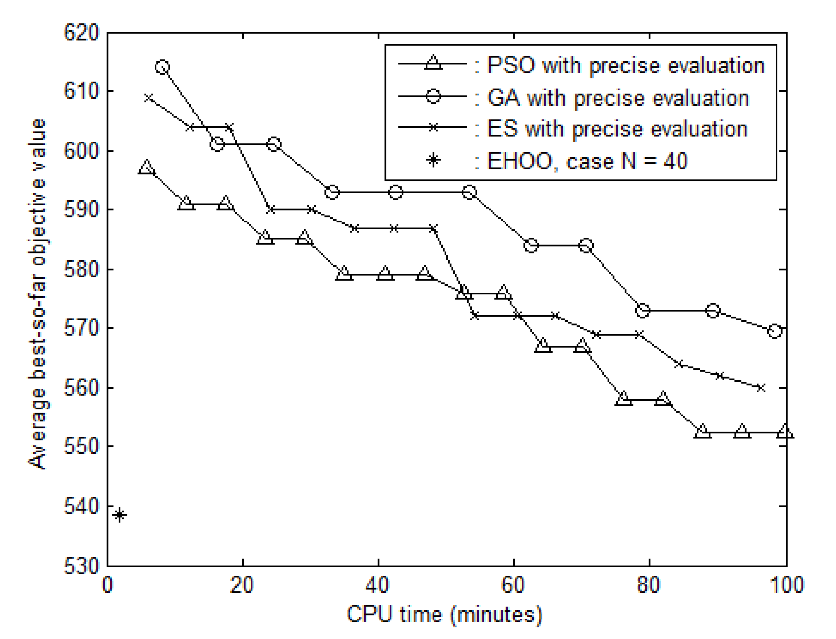
, solid line with circles Applsci 10 02075 i002, and solid line with crosses Applsci 10 02075 i003, respectively. Table 5 reveals that the average best-so-far objective values computed by PSO, GA and ES were 2.54%, 5.71% and 3.96% larger than that obtained by EHOO, respectively. The average best-so-far objective values determined by three competing approaches were worse not only than that obtained by EHOO with case N = 40, but also than those obtained by other three cases of N . Simulation results show that the EHOO approach can determine superb solutions in an acceptable time and outperforms the three competing approaches. As long as the three competing approaches continue to proceed for a very long time, it is reasonable to obtain better results than the proposed approach.

6. Conclusions

To resolve the SICOPs in an acceptable computation time, a heuristic method coupling EHO with OO was presented. The EHOO method has three parts including metamodel construction, diversification and intensification. The RMTS metamodel evaluated a solution vector in a short computing time. The EHOO method utilized the IEHO for diversification with the AOCBA for intensification. The EHOO method was applied to minimize the staffing cost in a one-period multi-skill call center, which was formulated as a SICOP. The EHOO method was compared to three optimization methods—PSO, GA and ES—with accurate evaluation. The superb solution that was resulted by the EHOO method had a high quality with favorable computing efficiency. Experimental results demonstrate that most of the objective values obtained by the EHOO method are close to the optimum in 30 individual runs. The EHOO method usually obtains a near optimum even though it does not provide a globally optimal solution. Future research will continue to focus on the improvement of OO method to resolve more complex stochastic optimization problems, such as portfolio optimization with stochastic dominance constraints and optimal reinsurance-investment problems.

Author Contributions

S.-C.H. conceived and designed the experiments; S.-C.H. performed the experiments; S.-S.L. analyzed the data; S.-S.L. contributed reagents/materials/analysis tools; S.-C.H. wrote the paper. All authors have read and agreed to the published version of the manuscript.

Funding

This research work is supported in part by the Ministry of Science and Technology in Taiwan, R.O.C., under Grant MOST108-2221-E-324-018.

Conflicts of Interest

The authors declare no conflicts of interest.

References

  1. Lejeune, M.A.; Margot, F. Solving chance-constrained optimization problems with stochastic quadratic inequalities. Oper. Res. 2016, 64, 939–957. [Google Scholar] [CrossRef]
  2. Lan, H.Y. Regularization smoothing approximation of fuzzy parametric variational inequality constrained stochastic optimization. J. Comput. Anal. Appl. 2017, 22, 841–857. [Google Scholar]
  3. Bhatnagar, S.; Hemachandra, N.; Mishra, V.K. Stochastic approximation algorithms for constrained optimization via simulation. ACM Trans. Model. Comput. Simul. 2011, 21, 15. [Google Scholar] [CrossRef]
  4. Hussain, K.; Salleh, M.N.M.; Cheng, S.; Shi, Y.H. On the exploration and exploitation in popular swarm-based metaheuristic algorithms. Neural Comput. Appl. 2019, 31, 7665–7683. [Google Scholar] [CrossRef]
  5. Yang, X.S.; Deb, S.; Zhao, Y.X.; Fong, S.M.; He, X.S. Swarm intelligence: Past, present and future. Soft Comput. 2018, 22, 5923–5933. [Google Scholar] [CrossRef] [Green Version]
  6. Ryerkerk, M.; Averill, R.; Deb, K.; Goodman, E. A survey of evolutionary algorithms using metameric representations. Genetic Program. Evolvable Mach. 2019, 20, 441–478. [Google Scholar] [CrossRef]
  7. Wang, G.G.; Deb, S.; Gao, X.Z.; Coelho, L.D. A new metaheuristic optimisation algorithm motivated by elephant herding behavior. Int. J. Bio-Inspired Comput. 2016, 8, 394–409. [Google Scholar] [CrossRef]
  8. Elhosseini, M.A.; el Sehiemy, R.A.; Rashwan, Y.I.; Gao, X.Z. On the performance improvement of elephant herding optimization algorithm. Knowl.-Based Syst. 2019, 166, 58–70. [Google Scholar] [CrossRef]
  9. Peska, L.; Tashu, T.M.; Horvath, T. Swarm intelligence techniques in recommender systems—A review of recent research. Swarm Evol. Comput. 2019, 48, 201–219. [Google Scholar] [CrossRef]
  10. Piotrowski, A.P.; Napiorkowski, M.J.; Napiorkowski, J.J.; Rowinski, P.M. Swarm intelligence and evolutionary algorithms: Performance versus speed. Inf. Sci. 2017, 384, 34–85. [Google Scholar] [CrossRef]
  11. Ho, Y.C.; Zhao, Q.C.; Jia, Q.S. Ordinal Optimization: Soft Optimization for Hard Problems; Springer: New York, NY, USA, 2007. [Google Scholar]
  12. Hwang, J.T.; Martins, J.R.R.A. A fast-prediction surrogate model for large datasets. Aerosp. Sci. Technol. 2018, 75, 74–87. [Google Scholar] [CrossRef]
  13. Tang, J.H.; Wang, W.; Xu, Y.F. Two classes of smooth objective penalty functions for constrained problems. Numer. Funct. Anal. Optim. 2019, 40, 341–364. [Google Scholar] [CrossRef]
  14. Horng, S.C.; Lin, S.S. Embedding advanced harmony search in ordinal optimization to maximize throughput rate of flow line. Arab. J. Sci. Eng. 2018, 43, 1015–1031. [Google Scholar] [CrossRef]
  15. Horng, S.C.; Lin, S.S. Embedding ordinal optimization into tree-seed algorithm for solving the probabilistic constrained simulation optimization problems. Appl. Sci. 2018, 8, 2153. [Google Scholar] [CrossRef] [Green Version]
  16. Horng, S.C.; Lin, S.S. Bat algorithm assisted by ordinal optimization for solving discrete probabilistic bicriteria optimization problems. Math. Comput. Simul. 2019, 166, 346–364. [Google Scholar] [CrossRef]
  17. Yu, K.G. Robust fixture design of compliant assembly process based on a support vector regression model. Int. J. Adv. Manuf. Technol. 2019, 103, 111–126. [Google Scholar] [CrossRef]
  18. Erdik, T.; Pektas, A.O. Rock slope damage level prediction by using multivariate adaptive regression splines (MARS). Neural Comput. Appl. 2019, 31, 2269–2278. [Google Scholar] [CrossRef]
  19. Sambakhe, D.; Rouan, L.; Bacro, J.N.; Goze, E. Conditional optimization of a noisy function using a kriging metamodel. J. Glob. Optim. 2019, 73, 615–636. [Google Scholar] [CrossRef]
  20. Han, X.; Xiang, H.Y.; Li, Y.L.; Wang, Y.C. Predictions of vertical train-bridge response using artificial neural network-based surrogate model. Adv. Struct. Eng. 2019, 22, 2712–2723. [Google Scholar] [CrossRef]
  21. Bouhlel, M.A.; Hwang, J.T.; Bartoli, N.; Lafage, R.; Morlier, J.; Martins, J.R.R.A. A Python surrogate modeling framework with derivatives. Adv. Eng. Softw. 2019, 135, 102662. [Google Scholar] [CrossRef] [Green Version]
  22. Hassanien, A.E.; Kilany, M.; Houssein, E.H.; AlQaher, H. Intelligent human emotion recognition based on elephant herding optimization tuned support vector regression. Biomed. Signal Process. Control 2018, 459, 182–191. [Google Scholar] [CrossRef]
  23. Kowsalya, S.; Periasamy, P.S. Recognition of Tamil handwritten character using modified neural network with aid of elephant herding optimization. Multimed. Tools Appl. 2019, 78, 25043–25061. [Google Scholar] [CrossRef]
  24. Meena, N.K.; Parashar, S.; Swarnkar, A.; Gupta, N.; Niazi, K.R. Improved elephant herding optimization for multiobjective DER accommodation in distribution systems. IEEE Trans. Ind. Inform. 2018, 14, 1029–1039. [Google Scholar] [CrossRef]
  25. Chen, C.H.; Lee, L.H. Stochastic Simulation Optimization: An Optimal Computing Budget Allocation; World Scientific: Hackensack, NJ, USA, 2010. [Google Scholar]
  26. Yu, M.; Chang, C.G.; Zhao, Y.; Liu, Y. Announcing delay information to improve service in a call center with repeat customers. IEEE Access 2019, 7, 66281–66291. [Google Scholar] [CrossRef]
  27. Ibrahim, S.N.H.; Suan, C.L.; Karatepe, O.M. The effects of supervisor support and self-efficacy on call center employees’ work engagement and quitting intentions. Int. J. Manpow. 2019, 40, 688–703. [Google Scholar] [CrossRef]
  28. Avramidis, A.N.; Chan, W.; L’Ecuyer, P. Staffing multi-skill call centers via search methods and a performance approximation. IIE Trans. 2009, 41, 483–497. [Google Scholar] [CrossRef]
  29. SimOpt.org, One Period, Multi-Skill Call Center. [Online]. 2016. Available online: http://simopt.org/wiki/index.php?title=Call_Center (accessed on 19 March 2020).
  30. Ryan, T.P. Sample Size Determination and Power; John Wiley and Sons: Hoboken, NJ, USA, 2013. [Google Scholar]
  31. Wang, Q.X.; Chen, S.L.; Luo, X. An adaptive latent factor model via particle swarm optimization. Neurocomputing 2019, 369, 176–184. [Google Scholar] [CrossRef]
  32. Delice, Y. A genetic algorithm approach for balancing two-sided assembly lines with setups. Assemb. Autom. 2019, 39, 827–839. [Google Scholar] [CrossRef]
  33. Spettel, P.; Beyer, H.G. A multi-recombinative active matrix adaptation evolution strategy for constrained optimization. Soft Comput. 2019, 23, 6847–6869. [Google Scholar] [CrossRef]
Figure 1. Framework of an regularized minimal-energy tensor-product spline.
Applsci 10 02075 g001
Figure 2. Flow diagram of the coupling elephant herding optimization with ordinal optimization approach.
Applsci 10 02075 g002
Figure 3. A one-period multi-skill call center consisting of J call types and K agent groups.
Applsci 10 02075 g003
Figure 4. Input output relationship in a one-period multi-skill call center.
Applsci 10 02075 g004
Figure 5. Variations of α and β over iterations.
Applsci 10 02075 g005
Figure 6. Progressions of four approaches over 30 individual runs.
Applsci 10 02075 g006
Table 1. Skill groups of the small problem.
Call Type λ j Agent Groups
14401 345 789 1112
2540 3 678 1112
3440 2 4 67 9101112
4540 5 10 12
5440 89101112
Table 2. Skill groups of the large problem.
Call Type λ j Agent Groups
12401 3 5 7 9
22401 11 13 15
3160 2 4 6 8 10
4260 4 12 14
513012 5 11
6230 3 78 10
7260 5 9 1213
8130 56 10 12 1415
9260 2 456 10
10125 56 9 1314
112351 5 8 10 12
12155 4 9 11 1415
13230 2 5 7 10 15
14260 3 89 13 15
15225 2 67 14
161301 5 10 12
17160 2 6 11
18130 34 1314
19260 2 8 12 15
20260 3 6 8 121314
Table 3. The superb solution x * , cost, service-levels and the CPU times in the small problem.
x * [17,18,17,16,18,17,16,17,16,16,17,17]T
g 0 ( x ) ~ g 5 ( x ) 0.80, 0.93, 0.86, 0.93, 0.51, 0.78
COST253.9
CPU time (sec.)24.67
Table 4. The superb solution x * , cost, service-levels and the CPU times in the large problem.
N x * Cost g 0 ( x ) CPU Times (sec.)
40[22,22,22,22,23,23,22,23,22,22,23,23,22,23,22]T5380.80115.65
30[23,22,23,22,23,22,22,23,23,22,23,23,22,22,22]T539.10.81112.34
20[22,22,23,23,23,22,23,23,22,22,22,23,22,23,22]T539.30.82109.51
10[22,23,22,22,23,22,22,23,22,23,23,23,22,23,22]T539.70.82107.47
Table 5. Comparison of the average best-so-far objective values of four methods over 30 individual runs.
ApproachesABO ABO § * × 100 %
EHOO, CASE N = 40538.60
PSO with accurate evaluation552.32.54%
GA with accurate evaluation569.45.71%
ES with accurate evaluation559.93.96%
ABO: Average best-so-far objective value; §: ABO obtained by EHOO.

