Article

Optimizing Inverse Distance Weighting with Particle Swarm Optimization

1
Department of Mathematics and Computer Science, Ovidius University of Constanta, 900527 Constanta, Romania
2
Department of Navigation and Naval Transport, Mircea cel Batran Naval Academy, 900218 Constanta, Romania
*
Author to whom correspondence should be addressed.
Appl. Sci. 2020, 10(6), 2054; https://doi.org/10.3390/app10062054
Submission received: 21 January 2020 / Revised: 9 March 2020 / Accepted: 11 March 2020 / Published: 18 March 2020
(This article belongs to the Special Issue Climate Change and Water Resources)

Abstract

:
Spatial analysis of hydrological data often requires the interpolation of a variable from point samples. Commonly used methods for solving this problem include Inverse Distance Weighting (IDW) and Kriging (KG). IDW is easily extensible, has a competitive computational cost with respect to KG, hence it is usually preferred for this task. This paper proposes the optimization of finding the IDW parameter using a nature-inspired metaheuristic, namely Particle Swarm Optimization (PSO). The performance of the improved algorithm is evaluated in a complex scenario and benchmarked against the KG algorithm for 51 precipitation series from the Dobrogea region (Romania). Apart from facilitating the process of applying IDW, the PSO implementation for Optimizing IDW (OIDW) is computationally lighter than the traditional IDW approach. Compared to Kriging, OIDW is straightforward to be implemented and does not require the difficult process of identification of the most appropriate variogram for the given data.

1. Introduction

Precipitation data analysis plays a major role in the process of making informed decisions for water resources management. Such data are gathered at monitoring stations scattered throughout a region. They are either not readily available for other locations or may be missing at certain time periods. These issues have negative influences on hydrological studies that rely on precipitation data as input. Therefore, spatial interpolation methods prove to be useful for estimating precipitation data at unsampled locations [1].
Spatial interpolation methods are commonly used for the prediction of the values of environmental variables. Their specificity comes from incorporating information related to the geographic position of the sample data points. The most used methods are usually classified in the categories [2,3]: (1) deterministic methods (Nearest Neighbor, Inverse Distance Weighting (IDW), Splines, Classification and Regression methods), (2) geostatistical methods (Kriging (KG)) or (3) combined methods (regression combined with other interpolation methods and classification combined with other interpolation methods).
The importance of a successful spatial interpolation of precipitation before the hydrological modeling and a thorough review of different spatial interpolation methods for its modeling are presented in [1]. Among them, IDW stands out as a real competitor. It builds estimates for environmental variables at a location, based on the values of those variables at some nearby sites and on the distances between that location and those where the variable is known.
The interpolation method often chosen by geoscientists is IDW, implemented in many Geographic Information Systems (GIS) packages [4]. Its popularity is mainly due to its straightforward interpretability, easy computability and good prediction results. Still, the No Free Lunch theorem for optimization [5] stands also in the case of spatial interpolation: no method stands out as being the best in all situations [6]. In a study about the rainfall data in the Indian Himalayas, Kumari et al. [7] performed a comparison of several interpolation methods, among which there were several variants of multivariate Kriging and IDW. It was shown that none of the methods performs best in all the studied cases. Principal Component Regression with the Residual correction (PCRR) method, IDW and the Multiple Linear Regression (MLR) methods were used to compare interpolated annual, daily and hourly precipitation and the spatial distribution of precipitation in the Xinxie catchment [8], while the spatial distribution of precipitation deficit over Seyhan River basin using IDW is reported in [9].
The basic IDW method is successfully employed in [10] to estimate the rainfall distribution in a region of Iraq. The scenario uses incremental values for the power parameter, in the range from 1 to 5. A modified IDW method is investigated in [11], where the elevation is also considered for estimating the values at unknown locations. A new method for estimating the regional precipitation (MPPM) has been introduced in [12] and its performance has been tested against that of IDW and kriging. It was reported that MPPM avoids the problems that could appear in the application of kriging methods, as (i) the invertibility of the distance matrix, (ii) the high computational cost related to building the inverse of the distance matrix in the case of a high number of stations, (iii) the choice of the model for the estimation of theoretical variogram and (iv) the selection of the optimal parameters of the variogram model. It was shown that deterministic methods could be good competitors for spatial interpolation techniques, such as KG, performing better than the last ones in the study cases presented in [12]. In an engineering setting, Gholipour et al. [13] investigate a hybridization of IDW with a harmony search. The obtained metamodel significantly reduces the computational effort and improves the convergence rate. A genetic algorithm is used in [6] to find the optimal order of distances in IDW.
An adaptive version of the IDW method is introduced in [4], where the authors suggest that the spatial pattern of the sampled stations in the neighborhood could influence the weighting parameter. The algorithm selects the weights in IDW based on the stations’ density around the unsampled location. It gave better estimations than KG on the study cases. However, the choices of the membership functions and the number of relevant neighbors are heuristics, and there is no guarantee that they will perform well in other scenarios.
Some machine learning models were also investigated in [3], with application to spatial interpolation of environmental variables. They are compared with several traditional spatial interpolation methods, among which is inverse distance squared. The study found that the combination of random forest and IDW, respectively random forest with OK were the best methods, with similar accuracies. At the same time, OK was found to perform similarly to IDW in the tested scenarios. A hybrid method that combines IDW with support vector machines is reported in [14], applied to multiyear annual precipitation. In [15], temporal predictions obtained with an ensemble approach are used as inputs to spatial interpolation by IDW, with improved overall results.
The main difficulty faced when applying IDW is setting the value of the power parameter. This is usually done before the algorithm is applied. The usual approach for searching for the optimal value of the power parameter is by exhaustive search, by sampling all possible values in a given interval, at a user chosen step size [2]. The results of this method depend on the search window. The method is only guaranteed to find a local optimum [2].
In this paper, we target the optimization of the process of setting the power parameter in IDW, using a nature-inspired metaheuristic—Particle Swarm Optimization. We automate the process of identifying the suitable parameter, while maintaining, if not optimizing, the prediction accuracy of the standard IDW method. Experiments are performed on maximum annual precipitation data gathered in the Dobrogea region (Romania). An evaluation of the proposed hybrid method is performed, against standard IDW and Kriging.
The paper structure is the following. 
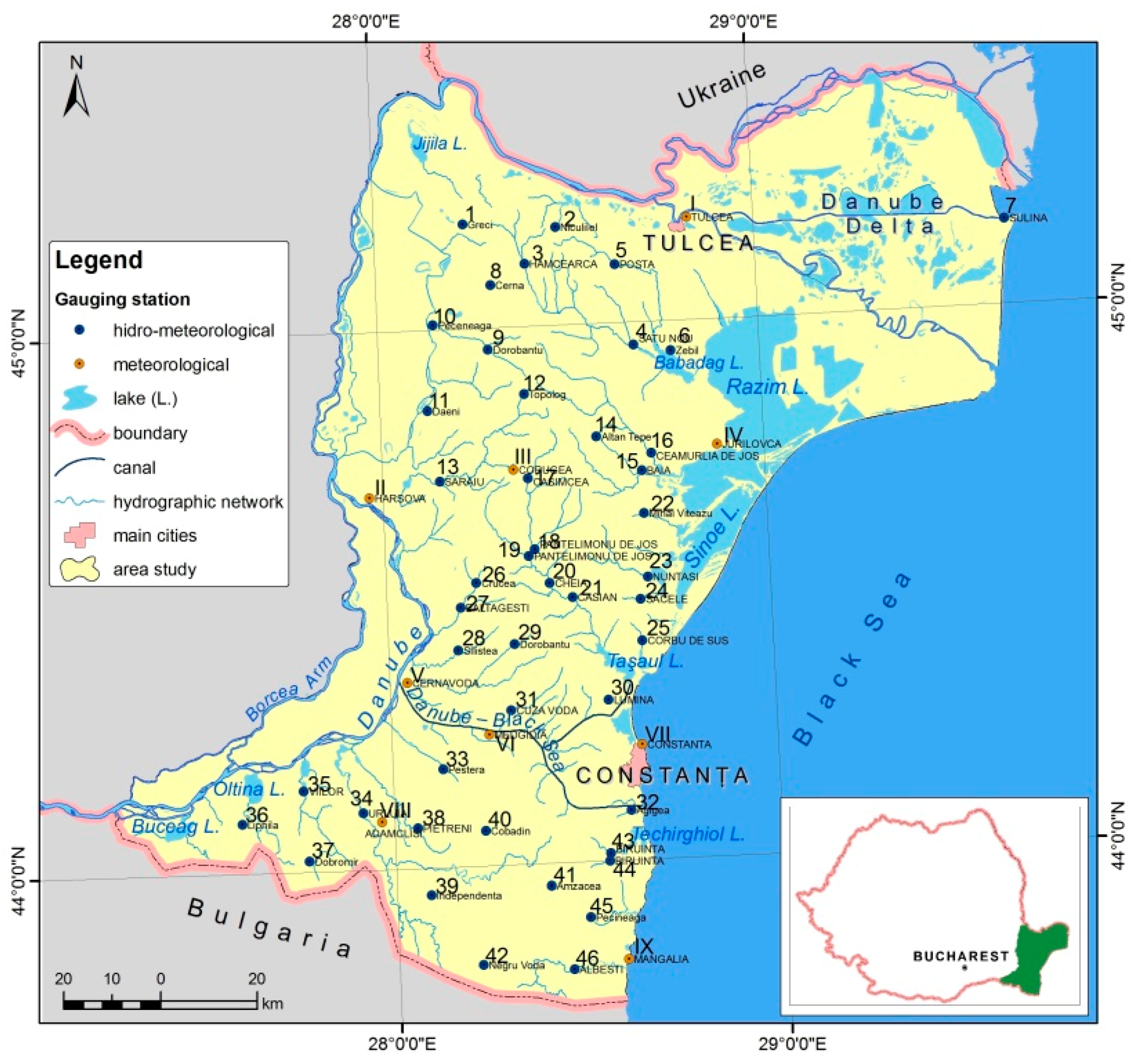
Section 2 begins with a brief presentation of the meteorological stations locations in the study area. Section 2.2 and Section 2.3 present the spatial interpolation methods IDW and KG. The Particle Swarm Optimization (PSO) metaheuristic is presented in Section 2.4. The section ends with the presentation of the hybrid algorithm Optimizing IDW (OIDW), obtained by optimizing the β parameter of IDW with PSO. The experimental settings are described in Section 3, while the results are discussed in Section 4. The paper ends with the conclusion section.

2. Materials and Methods

2.1. Study Area

The studied area is Dobrogea, a region of 15,500 km2 located in the South-East of Romania, between the Danube River and the Black Sea, between 27°15′15″–29°30′10″ eastern longitude and 43°40′4″–45°25′3″ northern latitude [16]. Its geographic structure is that of a plateau with a hilly aspect, the altitude decreasing from north to south. The climate is temperate–continental, but the region is subject to drought and desertification [16,17].
The study data consists of 51 series of 1-day maximum annual precipitation registered during the period January 1965–December 2005 at 10 main meteorological stations and 41 hydro-meteorological points in the region of Dobrogea, Romania (Figure 1). When working only with the data recorded at the main stations, the input data will be a table with 41 rows and 10 columns (in the A1 and B1 scenarios presented in Section 3), while when working with all data, the input will consist of a table with 41 rows and 51 columns (in the A2 and B2 scenarios presented in Section 3). The data were collected at the stations under the National Authority Romanian Waters; they are without gaps and they are reliable. The maximum annual series collected at the main meteorological stations are represented in Figure 2.

2.2. IDW Interpolation

Essentially, all spatial interpolation methods compute weighted averages of sampled data, as estimations for unknown data [2,3]. Given a set of spatial data of an attribute z at n locations, the general estimation formula is:
z ( s 0 ) ^ = i = 1 n w i ( s 0 ) · z ( s i )
where z ( s 0 ) ^ is the interpolated value estimated for the variable of interest at the station s 0 , z ( s i ) is the sample value at the station s i , w i ( s 0 ) is the weight attached to the station s i and n is the stations’ number.
The main difference between all spatial interpolation methods relies in computing the weights w i used in the interpolation.
The problem we tackled consists of estimating precipitation values for some locations where these values are unknown, using as input data the precipitation values recorded at several locations in the neighborhood. The general Formula (1) is also valid for IDW. The simplest version of weights estimation uses the inverse distances from all the points to the target one [18]:
w i ( s 0 ) = 1 / d ( s 0 ,   s i ) β i = 1 n ( 1 / d ( s 0 ,   s i ) β ) ,   β > 1 ,
where d ( s 0 ,   s i ) is the distance from s 0 to s i and β is a parameter that must be determined. Thus, the weights decrease as the distance increases, especially if the value of β is large. The parameter β determines the degree of influence the neighboring stations have upon the estimates for a given station (it is expected that nearer neighbors have more influence upon the estimated value than the more distant ones).
Choosing β is an optimization process by itself. Usually, the search for the optimal β is a grid search: a specific range is set (arbitrarily or based on some intuition of the researcher), and then β takes all values in that range, with a certain step-size, also arbitrarily chosen. The value yielding the lowest prediction error (among the searched values) is finally attributed to the parameter.

2.3. Kriging

Kriging (KG) is the generic name given to a family of generalized least-squares regression algorithms, used in geostatistics for data spatial interpolation. The spatial correlation was analyzed in geostatistics using the variogram. The main ideas behind the methodology for Kriging are shortly presented below, based upon the bibliographic resources [19,20].
Given a random function Z(s) that is stationary, with a constant mean E(Z(s)) = μ, the semivariogram is defined by:
γ ( h ) = 1 2 E ( Z ( s i ) Z ( s i + h ) ) 2 ,
where Z( s i ) and Z( s i + h ) are the variable values at the study station and at a location situated at the distance h from the study location. When assuming the direction independence of the semivariance (isotropy), the variogram can be estimated using ∑ the sample variogram, defined by
γ ^ ( h ) = 1 2 N h i = 1 N h ( Z ( s i ) Z ( s i + h ) ) 2
where N h is the number of sample pairs ( Z ( s i ), Z ( s i + h ) ) used in estimation and where N(h) is the number of data pairs, which are approximately separated by the lag h.
After computing the sample variogram, one should determine the empirical semivariogram by fitting a parametric model to it. This can be done by the Generalized Least Squares (GLS), Maximum Likelihood or Bayesian methods [19]. GLS is the method used in this article.
The nugget, sill and range are the parameters used to describe a variogram (Figure 3). The nugget is the random error process, shown by the height of the jump of the semivariogram at the discontinuity at the origin. The sill is the variogram limit, when the lag tends to infinity. The range is the minimum lag at which the difference between the variogram and sill becomes negligible [21].
Different types of variograms may be used, as function of the data series, for example spherical, exponential, Gaussian, Matern and power [19].
At the final modeling stage of ordinary KG, the predictions are based on the model:
Z ( s ) = μ + ε ( s )
where μ is the mean and ε ( s ) is the spatially correlated stochastic part of variation. The predictions are obtained by formula:
z 0 ^ ( s 0 ) = i = 1 n w i ( s 0 ) z ( s i ) = λ 0 T z
where λ 0 T is the transposed KG weights vector (wi), and z is the vector containing the observations at n neighbor locations.
The Kriging predictions are obtained by:
z 0 ^ ( s 0 ) = i = 1 n w i ( s 0 ) z ( s i ) = w 0 T z
where w 0 T is the transposed kriging weights vector (wi), and z is the vector containing the observations at n neighbor locations. The weights are based on the covariances among points in the sample and the covariances between sample points and the point to be predicted. The Kriging estimator should be unbiased and the error variance is minimized.
The weights for ordinary Kriging can be found by solving the Kriging equations:
w = [ C 11 C 1 n 1 C n 1 C n n 1 1 1 0 ] 1 [ C 10 C n 0 1 ]
where C i j = Cov ( Z i , Z j ) ,   C i 0 = Cov ( Z i , Z 0 ) and λ is the Lagrange multiplier that appears due to the constraint i = 1 n w i = 1 .
Since the first step of the KG procedure is building a variogram (not a covariogram), one should want to determine the Kriging equation, in terms of variogram. Under the hypothesis of second-order stationarity:
C i j = σ 2   γ i j ,
σ 2 is the variance and γ i j is the semivariance. Therefore, (8) can be written in the equivalent form:
[ γ 11 γ 1 n 1 γ n 1 γ n n 1 1 1 0 ] [ w 1 w n λ ] = [ γ 10 γ n 0 1 ]
The generalized least squared (GLS) estimate of the global mean of the data in the study region is given by:
m ^ G L S = ( 1 T C 1 1 1 ) 1 1 T C 1 1 z
where 1 = (1, …, 1) and C 1 = [ C 11 C 1 n C n 1 C n n ] [22].
The KG goodness of fit is influenced by the spatial data structure, the variogram choice and the number of data points chosen for the computation [23]. KG is more reliable when the number of stations is big enough [24]. For details on different approaches to Kriging study, the readers may refer to [19,20,25].

2.4. Particle Swarm Optimization (PSO)

Metaheuristics are problem-independent (stochastic optimization) techniques [26]. They are strategies that guide the search process, for an efficient exploration of the search space, for finding near-optimal solutions. Metaheuristic algorithms are approximate and usually non-deterministic, and they usually find “good” solutions in a “reasonable” amount of time [27]. Their advantage is that they are noise tolerant; they do not need the source code of the evaluation simulation, which can be used as a black box.
Swarm Intelligence (SI) comprises a class of novel population based intelligent metaheuristics, inspired from the emergent intelligent behavior of flocks of birds, fish, ants, immune system, bacteria, etc. In such collectivities, social interactions lead to complex social behavior, and that behavior is modified in dynamic environments. Particle Swarm Optimization (PSO) represents a branch of algorithms of SI, which implements a computational model for social learning [28]. The algorithm works with a population of particles (swarm) that, initially, are randomly generated throughout the search space of the problem. The particles are evaluated against a fitness function, each of them searching for locations in the fitness landscape with better fitness values. Each particle has neighbors, with which it exchanges information, and which are dictated by the representation of the particle and the neighborhood topology.
The PSO algorithm consists in a swarm of particles that move in a (multidimensional) search space. Each particle has a position x, a speed v, a memory of its most recent success (pbest—personal best—the position where the particle has obtained the best fitness) and a memory of the best neighbor (gbest—global best—the particle with the best neighbor in the neighborhood). The particles’ speed and positions are updated after each iteration, according to the following equations:
v [ t + 1 ] = w 1 v [ t ] + w 2 rand ( ) + w 3 rand ( gbest x )
x [ t + 1 ] = x [ t ] + v [ t + 1 ]
The parameters that appear in Equation (5) are:
-
w 1 the inertia weight, which forces the particle to move in the same direction; it balances exploration and exploitation. When w1 is high, PSO is focused on the search space’s exploration. When w1 is small, PSO focuses on exploitation rather than on exploration. Scenarios in which w1 decreases in time are usually used;
-
w 2 and w 3 the learning factors—they are weights of the acceleration that attracts the particle towards its personal best position or the global best position. w 2 is the cognitive learning factor, that suggests the tendency to repeat personal actions that proved more successful, while w 3 is the social learning factor—a measure of the tendency to follow the success of the best individual from its neighborhood.
After updating the speed, a speed limitation rule is usually applied, to prevent the particles from moving chaotically in the search space:
v [ t + 1 ] = max ( v max ,   min ( v max , v [ t + 1 ] )
where v max is a parameter of the algorithm.
The basic structure of the PSO Algorithm 1 is the following:
Algorithm 1
1: t = 0;
2:   Create the initial swarm P(0)
3:   repeat
4:    Evaluate particles in P(t) using the fitness function
5:    Update pbest for each particle
6:    Update gbest
7:    t = t + 1;
8:     foreach particle in P(t)
9:      Update its speed using Equation (12)
10:      Update its speed using Equation (14)
11:     Update its position using Equation (13)
12:    end foreach
13:   until stopping criterion is met

2.5. Optimization of the IDW Parameter with PSO

The optimization we propose is to identify the value of the optimal β, from (2) using PSO as the search algorithm. The PSO metaheuristic was chosen due to its simplicity with respect to coding, small computational cost and reduced number of parameters (by comparison with genetic algorithms, for example). PSO’s documented success in optimization applications in a wide range of engineering problems [28,29] was also a decisive factor in choosing PSO over other metaheuristics.
The particles’ positions in the PSO algorithm encode candidate solutions for the power parameter in Formula (2) of the IDW weights. They are randomly generated initially within the interval [1.0001, 5] (since β > 1, from the IDW definition).
The fitness function used in the algorithm assigns to each particle the mean squared error (MSE) of the predictions made with IDW, using as weight the power parameter β encoded by the respective particle:
fitness ( β ) = 1 n i = 1 n ( p i m i ) 2
where:
  • n is number of stations used in the IDW,
  • p i is the value predicted by IDW for the precipitation at station i,
  • m i is the (known) measured value for the precipitation at station i.
As far as we know, the proposed approach is new in the literature.
In the following we will refer to the improved algorithm as Optimized IDW (OIDW). Figure 4 presents the flowchart of the OIDW algorithm.

3. Experimental Settings

The experiments were run using an improved deterministic PSO variant from [30], which is among the most popular versions of the PSO algorithm [31]. We are interested in assessing the quality of predictions for OIDW and compare them with the traditional grid search IDW (denoted, in the following. by IDW*).
The experiments were run in 2 scenarios:
(Scenario A)
First, we used PSO and grid search to identify a single β that minimizes the sum of prediction error over all stations. The β value identified is characteristic of the entire Dobrogea region, hence it can be useful to infer values at points where no recordings are available, for example. When the predicted values for a given station are computed, the weights in Formula (1) corresponding to that station are set to 0.
(Scenario B)
We used PSO and grid search to search a β for each station that minimizes the prediction error when the series from that station is estimated using the other series from the other stations.
For example, if we have ten stations, to estimate the precipitation at the station I, the series recorded at the stations II-X are used as input, while the series recorded at the station I are hold out as control values. Thus, they are used for comparison with the values computed by applying Formula (2) with the parameter β1 identified by OIDW. The β1 obtained minimizes the MSE for the station I. Another example: to estimate the values of the series from the station V, the series recorded at station I-IV and VI-X are used as an input, and a β5 is computed, corresponding to the minimum MSE for the station V, and so on.
Further, we refined the experimental settings by performing experiments in two stages. First, we employed a reduced dataset comprising the series from ten main meteorological stations. We will refer to these scenarios as (A1) and (B1). The same experiments were repeated with the extended dataset that contains all 51 series. We will refer to these scenarios as (A2) and (B2). Hence we obtained four scenarios. We took a special interest in type (A) experiments because they should yield a unique empirically determined β to be characteristic for the entire region.
For each scenario, 50 different runs of the PSO algorithm were performed. The default Mersenne twister randomizer with an initial seed of 0 was used in the experiments reported in the tables below.
Setting the PSO parameters to optimal values is a very difficult optimization problem by itself [30,32]. In our experiments, the PSO parameters are chosen to match those widely used in the literature [30]:
  • The swarm size is 24,
  • Personal best influence is 2,
  • Global best influence is 2,
  • The inertia weight, decreasing during the iterations of the algorithm from 0.9 to 0.4,
  • The number of epochs (i.e., PSO iterations) is 100,
  • β is searched in the interval (1, 5).
The results are compared with those obtained by applying IDW and KG. For IDW, we identified the parameter β performing a grid search with the step-size of 10−4, in the interval [1.001, 5]. The grid search identifies the parameter β that yields the minimum prediction error (that will be listed in the results tables).
The experiments for OIDW and IDW* were performed in the Matlab environment, in Matlab R2012, on a computer with Intel Core i5 quad-core processor at 2.30 GHz with 8 GB RAM, using the PSO toolbox, available online [33]. Matlab was also used for performing the IDW* computation (IDW with the grid search).
For KG, we used Ordinary Kriging and report the mean prediction error obtained. The Kriging algorithm was run using the gstat, sp, spacetime, automap and geoR libraries from the R software. Different types of variograms (spherical, exponential, Gaussian, linear and power) were fit to the data, using autofitVariogram (from automap package) [34] and the best one (in terms of the lowest MSE) was selected. While for using the fit.variogram function (from gstat package) [35] the user has to supply an initial guess (estimate) for the sill, range, etc. to fit a certain type of variogram, the use of the autofitVariogram function (from automap package) does not necessitate any initial guess. autofitVariogram has the advantage to provide this estimate by computing it based on the data, and then calls the fit.variogram function [35]. So, 
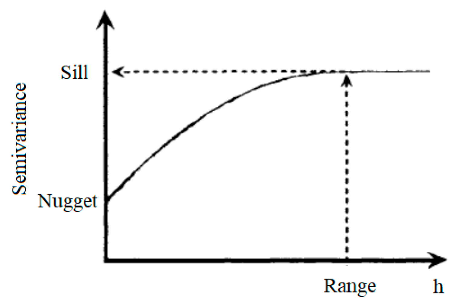
autofitVariogram automatically provides fit parameters (sill, nugget and range) of the best variogram. For a deeper insight on the variogram fitting, one can see the vignettes of the mentioned packages on the website of R software [34,35]. In our case, the fit variogram was of an exponential type, with the parameters sill = 144.9766 and range = 48,843.73.
To check if the MSE obtained in OIDW (A and B scenarios) and IDW* are not statistically different, the following statistical tests have been performed:
● The Anderson–Darling test [36], for testing the null hypothesis of data series normality:
The series is Gaussian (has a normal distribution),
Against the alternative that:
The series is not Gaussian (has not a normal distribution).
● The Levene’s test [36] for verifying the null hypothesis that:
The MSE series (from the scenarios A, B and IDW*) have the same variance,
Against the alternative that:
The MSE series do not have the same variance;
● The non-parametric Kruskal–Wallis test [37], for checking the null hypothesis that:
The mean ranks of the groups of MSE series (from the scenarios A, B and IDW*) are the same.
Against the alternative:
The mean ranks of the groups are not the same.
● The non-parametric eqdist.etest test [38], for verifying the null hypothesis that:
The MSE series (from the scenarios A, B and IDW*) have the same distribution,
Against the alternative:
The MSE series did not have the same distribution.
These nonparametric tests were selected because the normality hypothesis was rejected for some MSE series in A, B scenarios and IDW*. These tests were performed at the significance level of 5%, using the R software, version R 3.5.1.

4. Results and Discussion

The experimental results of the study are presented in Table 1, Table 2, Table 3 and Table 4, which contain:
β values rounded up to 4 decimals (which are mean values for the β’s obtained over the 50 runs of the PSO algorithm);
Standard deviations of the computed β values, denoted by st.dev.;
Mean squared errors (MSE) of the series values obtained in the experiments. The MSE is the average squared difference between the estimated values and the actual values; it is a measure of a model’s quality (Formula (15)). The smaller the MSE, the better the model is.
The time (in seconds) for running an experiment in the case of IDW*;
The average run time (in seconds) over all the 50 experiments and the standard deviation of the time in the OIDW experiments.
PSO is a stochastic algorithm; hence, mean and standard deviations are reported for both the optimized parameter, and the time consumed by the algorithm. The standard deviation is a proof of the algorithm stability (i.e., when the standard deviation is very small it means that the algorithm converges in every run; hence, it is stable and reliable).
The results obtained using only the series recorded at the ten main stations in the experiments done in the scenario A1 are displayed in Table 1, as follows: IDW* (columns 2–4), OIDW (columns 5–7) and KG (column 8). The values of the β parameter are equal up to the fourth decimal in IDW* and OIDW. The average run time for IDW* is 82.19 times greater than that for running OIDW (column 4-60 s and column 7-0.73 s).
Table 2 displays the results of the experiments performed using the series recorded at the main meteorological station, in the scenario B1.
We remarked that the PSO convergence was very good. The standard deviations of time and β in the OIDW algorithm are of the order of 10−4, respectively 10−6, hence they are not reported individually in the table. The values identified by OIDW coincide with those identified by IDW*, by the 4th decimal. A significant difference appears in the computational time. In the scenario B1, the average computational time for an OIDW run is more than 60 times smaller than the time for a IDW* run.
In both scenarios (A1 and B1), OIDW found the optimum, as it was exhaustively identified by IDW. Moreover, the differences between the mean squared errors of the approximations computed with IDW using the β values identified with grid search (IDW*) and OIDW were not statistically significant. Additionally, the MSEs associated to the IDW algorithms are almost identical; in some cases, these are better than those obtained by KG. The standard deviations of β are very small in both scenarios. This signifies that the PSO search for β is stable—PSO converged in all the 50 runs to very similar values. The average MSE are 30.9327 for IDW* and OIDW in scenario A1; 30.3704 for IDW* and 30.3718 for OIDW in scenario B1 and 31.022 for KG, respectively (Table 1 and Table 2). It was expected that OIDW in the scenario A1 (Table 1) would yield larger prediction errors than the individual OIDW’s in the scenario B1 (Table 2), since in B1 the algorithm tries to fit a much smaller number of data points.
Nevertheless, the differences with respect to KG are significant only in one case (e.g., Adamclisi). OIDW is run for each station in scenario B1, hence the computational times in Table 2 add up, for a fair comparison; OIDW is run only once for the entire set in A1, with the time as reported in Table 1. Therefore the time to run the experiments in scenario B1 is smaller than in A1 (1.31 times in for IDW* and 1.66 times for OIDW).
Table 3, Table 4, Table 5 and Table 6 contain the results obtained in experiments performed using the 51 meteorological stations, in scenario A2 and B2, respectively. Results in Table 3 prove that PSO converges to the optimal β, as it was identified by grid search (standard deviation of 1.1813 × 10⁻⁴).
For the main stations, the standard deviations are equal up to the third decimal for almost all the series. The computational effort, reported as run time, was significantly smaller (40 times) in the case of the OIDW algorithm (190 s for IDW* and 4.846 s for OIDW). The average MSE computed in A2 experiments were the following: 30.64324 (IDW*), 30.64315 (OIDW) and 30.876 (KG)—computed using the MSE for the main series; 31.0671 (IDW*), 31.0671(OIDW) and 29.5480 (KG)—computed using the MSE for the 41 secondary series and 30.9840 (IDW*), 30.9840 (OIDW) and 29.7924 (KG)—computed using all series. We found that the average MSE was smaller in all situations in scenario A2 for the main series, by comparison to scenario A1. The smallest average MSE in scenarios A1 and A2 corresponded to KG, when extracting only the secondary series (followed by the case when using all the series) for the MSE computation.
The results from Table 5 reveal little to no difference between the β’s identified by grid search and those identified by PSO search. Therefore, the MSE’s associated to the computed IDW approximations were identical. The significant difference comes from the computational time: PSO identified the optimal value 50 times faster than the grid search.
The MSE’s in scenario B2 are smaller in the experiments with 51 stations than those in the experiments with only ten main stations.
In scenario B1, when taking into account only the results for the main stations, they were as follows: 30.3704 vs. 29.22245 for IDW*, 30.37178 vs. 29.22245 for OIDW and 31.022 vs. 30.876 (Table 7, rows 3 and 6). This was to be expected because the algorithms received far more information in the scenario B2 than in B1. On the other hand, from the same reason, β st.dev in OIDW increased, while remaining very small.
All the results from Table 7 that summarizes the average MSE in all experiments show similar performances of IDW*, OIDW and KG. None of the algorithms were the best in all situations, confirming the literature findings [39].
Therefore, one can remark that OIDW yields competitive results in terms of MSE’s of estimated values when compared to KG. This is important because it proves OIDW to be a reliable method.
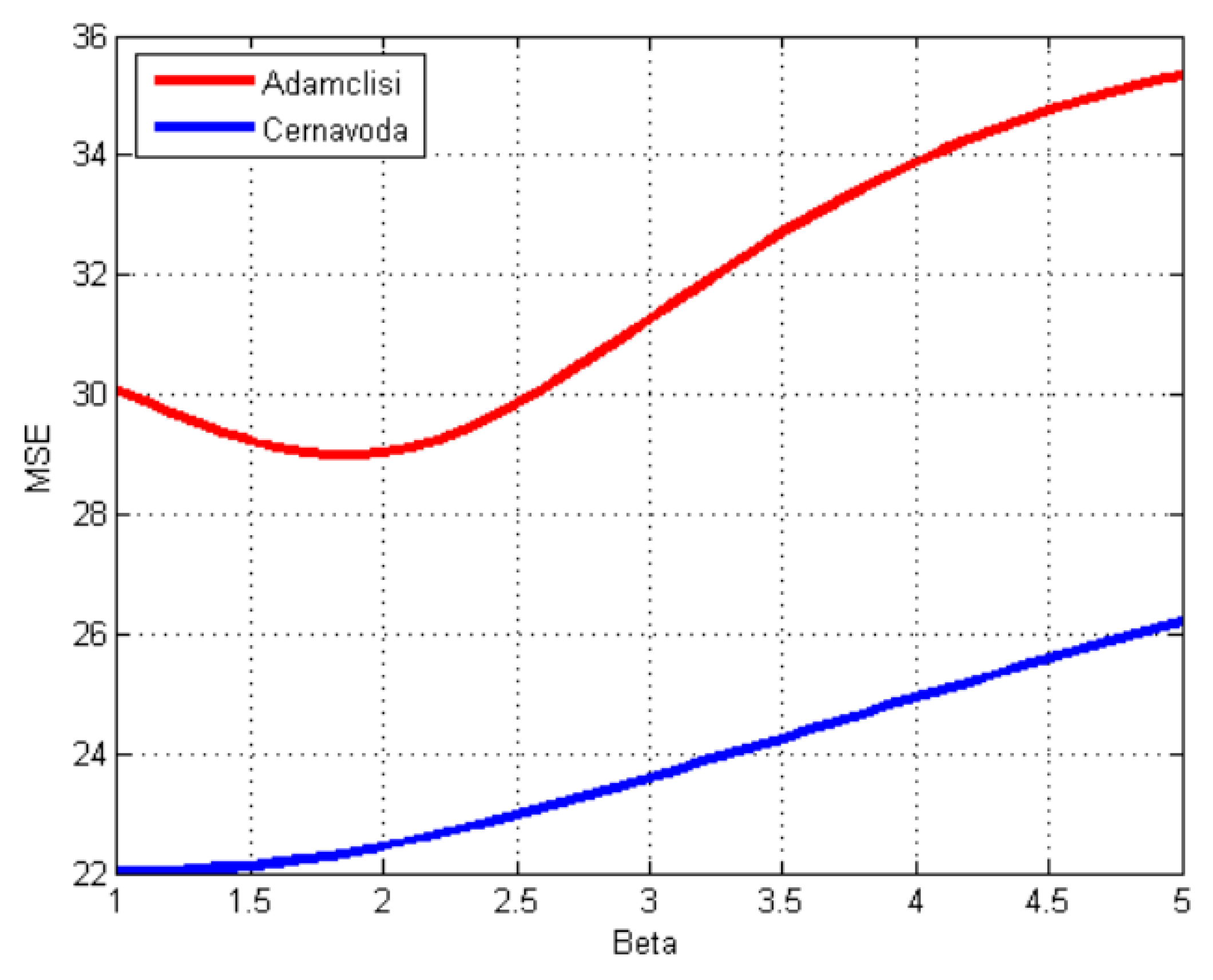
Finding the minimum MSE in the grid search is not straightforward because the MSE evolution patterns are different, as it is illustrated in Figure 5, for two series, where the MSE is computed using all the series, with a grid search step of 10−4. For Cernavoda, the trend is almost linear, while for Adamclisi, it decreases them it increases and presents an inflexion point. 
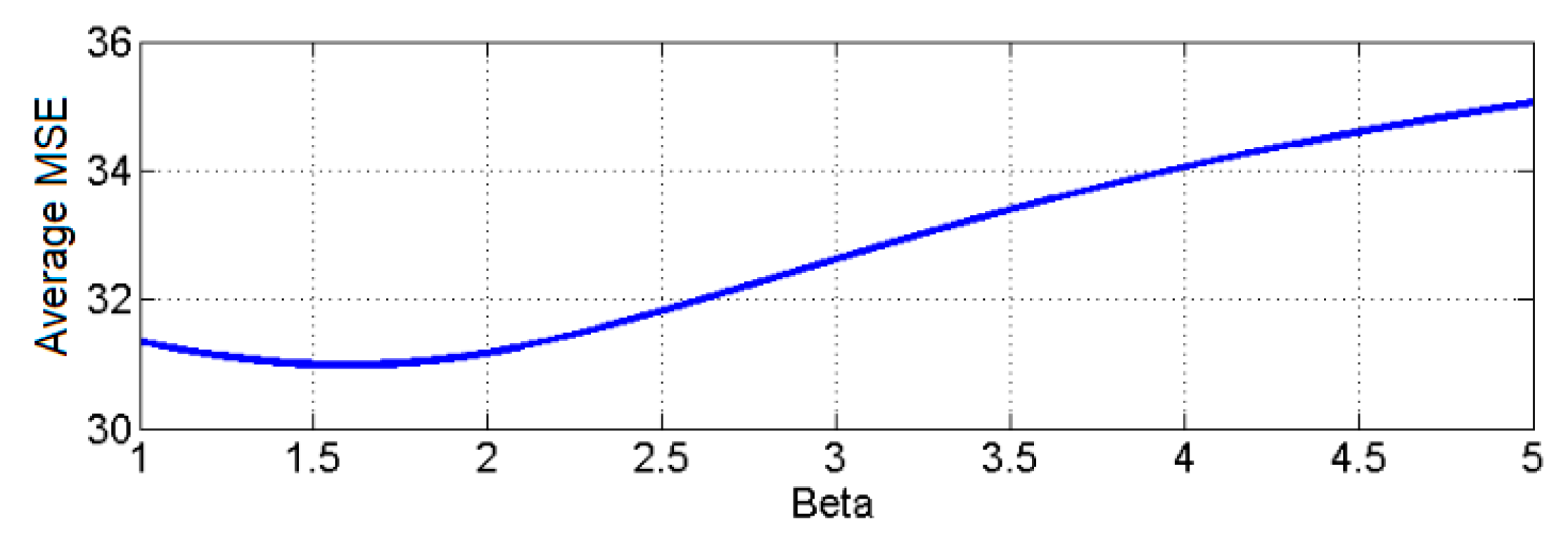
Figure 6 depicts the dependence of the average MSE for all series as a function of β. The chart has a similar behavior as for the Adamclisi series.
With respect to computational effort: for detecting the β that minimizes the MSE for fitting the values of a series in IDW* using a grid search with a step r, on an interval [a. b], the computation should be performed [ ( b a ) / r ] + 1 times (where [] is the integer part of the number inside the bracket). For example, for a grid search with a step of 0.1, IDW* was performed 50 times for each station, so 500 times when only the main stations were employed and 2550 times when all the 51 series were used.
Once again, taking into account the consumed time in scenarios A1 or A2, B1 or B2 is more convenient to run OIDW. This idea is supported by the fact that the β’s identified with OIDW in all the runs were identical to optimal values of β found by grid search IDW* up to the third digits (so, OIDW converged to a global optimum, in all cases).
OIDW performed better than KG in 60% of cases in scenario A1, in 80% of cases in scenario B1, and in 49.01% cases in scenarios A2 and B2. While in the scenarios A1 and B1, the OIDW MSE and KG MSE are comparable, in the A2 and B2 scenarios, there are some discrepancies between them, as for example, for Sulina, Cheia, Negureni, Pantelimon and Mihai Viteazu (in A2 and B2). This situation could be explained by the following reasons: (a) the low number of series used in A1 and B1 scenario, (b) the inhomogeneity of the stations on the in the Dobrogea region, (c) the climate differences on the different part of the region and (d) the possible anisotropy was not considered.
The results of the statistical tests on the SE series for OIDW and IDW* are presented in the following. The normality test for the MSE series corresponding to the experiments in scenarios A1, B1, OIDW, KG and IDW* from Table 1 and Table 2, A2, B2, IDW*, KG from Table 3 and Table 5, KG from Table 3 + Table 4 and KG from Table 5 + Table 6 could not reject the normality hypothesis. The same test led to the normality rejection for the IDW* MSE and OIDW MSE series corresponding to the secondary stations from Table 4 and Table 6, but not for OIDW MSE corresponding to all the series in Table 3 + Table 4 and Table 5 + Table 6.
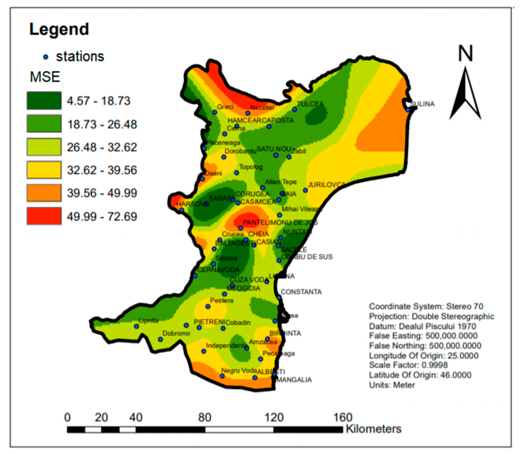
A spatial map containing illustration the distribution of MSE in OIDW form B2 scenario (values from Table 5 + Table 6) is presented in Figure 7. The highest MSEs correspond to the station near the region border, where the stations had few close neighbors.
To offer a different perspective of the OIDW performance, we computed the Mean Absolute Percentage Error (MAPE) and the Kling–Gupta efficiency (KGE).
The MAPE is given by the formula:
MAPE = 1 n i = 1 n | p i m i m i |
where n is number of stations used in the IDW, p i is the value predicted by IDW for the precipitation at station i and m i is the measured value for the precipitation at station i.
The KGE coefficient is introduced in [40]; it is defined by formula:
KGE = 1 − ED
where:
ED = ( r 1 ) 2 + ( σ s σ 0 1 ) 2 + ( μ s μ 0 1 ) 2
where μ s is mean of the values resulted from the model, μ 0 is the mean of the recorded values, σ s is the standard deviation of the values resulted from the model and σ 0 standard deviation of the recorded values.
MAPE is a scale-independent indicator that could be used in order to compare the performance of a given method on separate data sets. The lower MAPE is, the better the model is. The KGE coefficient is dimensionless as well and has an ideal value of unity. Although, in this study, the models were calibrated using the MSE as the model calibration criterion, the KGE and MAPE provide further validation of the obtained models.
Table 8 provides the MAPE values together with the Root Mean Square Errors (RMSE = MSE ) and the KGE for the ten main stations.
Similar results for MAPE and KGE were obtained in the A2 and B2 scenarios, so we are not presenting them here.
The highest MAPE value (so the worst data fit) was noticed for the Sulina station in both scenarios. It was expected, since Sulina is situated 12 km offshore, in the Danube Delta, and the climate presents different particularities compared with the rest of Dobrogea region. The same was true for the KGE coefficient: its lowest values were obtained for the Sulina and Mangalia stations (the most isolated stations).
Since the values of both goodness-of-fit indicators, dimensional-RMSE and dimensionless-MAPE are small, and most of the KGE values are bigger that 0.5, it resulted in the OIDW performing well.
The Levene’s test could not reject the hypotheses that groups of MSE from Table 1, Table 2, Table 3 and Table 4 (together), Table 5 and Table 6 (together) and Table 3, Table 4, Table 5 and Table 6 were homoskedastic, the corresponding p-values associated to this test were greater than the significance level of 5%.
The Kruskal—Wallis test could not reject the null hypothesis, the corresponding p-values being 0.9356 (Table 1 and Table 2), 0.8348 (Table 3 + Table 5), 0.6437 (Table 4 + Table 6) and 0.7519 (Table 3, Table 4, Table 5 and Table 6 all the stations), respectively. The eqdist.etest test applied to the same groups of series as in the previous test could not reject the hypothesis that each group of series has the same distribution, the corresponding p-values being greater than the significance level of 5%.
Concluding, the MSE’s of the estimations obtained by OIDW, IDW* and KG were not significantly different.
When KG is not very straightforward to be applied and searching for the best parameter β for IDW with grid search is computationally intensive, OIDW proves to be a convenient and rapid to use solution.
Other optimization methods can be applied for the power parameter of IDW calibration, such as methods based on the Golden Section (GS) method, provided that the hypotheses of this method are satisfied. As an example, we tried to calibrate the parameter β by this additional optimization method, namely by the fminbnd Matlab function [41]. This function applies GS, followed by parabolic interpolation; the boundaries for the search are to be specified as parameters. In the experiments performed on the series from the ten main stations with the fminbnd method, we obtained an approximation of 1.1903 f or β with a duration of 1 s, with MSE = 30.75. The results are comparable in this situation with those obtained by both OIDW and IDW. The assumptions for this method include that the function to be minimized should be continuous, which is hardly the case in real world problems. Additionally, since in some situations the fminbnd fails to find the optimum (as in the case of independent stations, where there are local minima or when minimum lies on the boundary of the search domain [41]), we consider that an extensive study should be done to compare our approach with that of fminbnd. The results will be communicated in another article.

5. Conclusions

The paper describes a hybrid PSO-IDW algorithm for the modeling of data; it is applied on maximum precipitation data in the experimental part. The algorithm is based on a well-known spatial interpolation method (IDW). Since the application of IDW makes use of the power parameter β, we proposed the use of the PSO algorithm to identify a suitable value for this parameter. Empirical results proved that the IDW performance was maintained, while the new method offered lower computational costs. Results of the IDW and OIDW were further compared to Kriging.
The optimization of IDW with PSO described in this paper offered an alternative to an exhaustive search for the problem of tuning the power parameter in the IDW method. In cases when the estimations provided by the traditional application of IDW are good, the results obtained with OIDW should preserve the quality of the prediction and be better in terms of computational effort.
Kriging is a powerful geostatistical method, suitable to be applied in certain cases, and its application assumes profound knowledge of spatial statistics. When the spatial correlation is strong and the variogram can depict well the spatial variability, the KG algorithm predicts very well. Even so, for our precipitation data, the results are not substantially better by KG, as it was the case for other environmental variables studied in [17]. In cases where the nature of the input data does not support KG, instead of using IDW for prediction it is wiser to choose OIDW since it automates the process of identifying the appropriate power parameter, with smaller computational effort. Our approach also benefits from the advantages of the PSO algorithm: a simple implementation, robustness, small number of parameters to adjust and a high probability and efficiency in finding the global optima, fast convergence, short computational time and modeling accuracy. OIDW is easy to use by people that do not have statistical knowledge [29,42].
The limitations of IDW are preserved by OIDW: in locations with sparse neighbors (such as those near the borders of the study region), the errors for IDW simulated data are larger. While providing a solution for optimizing the IDW parameter, OIDW uses PSO, which has several parameters of its own that need to be set (e.g., swarm size, the weights in the Equations (7) and (8)). In our experiments, setting these parameters to values commonly used in the literature led to very good results.
The contribution of our paper was two-fold. For hydrologists, we introduced an optimization of a well-known and widely used spatial interpolation method—namely IDW. For the artificial intelligence community, we proved the utility of the application of the PSO metaheuristic on a parameter optimization problem.
The results obtained in our case study using time series data from 51 meteorological locations in the Dobrogea region (Romania) encouraged us to consider OIDW as a good choice for the spatial interpolation of precipitation data. Still, more experiments will be performed, using various types of environmental data and various measures of performance of the models, in order to decide the appropriateness of OIDW as a general spatial interpolator.

Author Contributions

Data curation: A.B. (Alina Barbulescu); Investigation: A.B. (Alina Barbulescu) and A.B. (Andrei Bautu); Methodology; E.B.; Software: A.B. (Andrei Bautu); Supervision: A.B. (Alina Barbulescu); Writing original draft: A.B. (Alina Barbulescu) and E.B.; Writing—review and editing: A.B. (Alina Barbulescu) and E.B. All authors have read and agreed to the published version of the manuscript.

Funding

This research received no external funding.

Acknowledgments

We thank the anonymous reviewers for the very useful comments and insights offered in the reviews. Our paper was significantly improved by taking into account their observations.

Conflicts of Interest

The authors declare no conflict of interest.

References

  1. Ly, S.; Charles, C.; Degre, A. Different methods for spatial interpolation of rainfall data for operational hydrology and hydrological modeling at watershed scale: A review. Biotechnol. Agron. Soc. Environ. 2013, 17, 67–82. [Google Scholar]
  2. Li, J.; Heap, A.D. Spatial interpolation methods applied in the environmental sciences: A review. Environ. Model. Softw. 2014, 53, 173–189. [Google Scholar] [CrossRef]
  3. Li, J.; Heap, A.D.; Potter, A.; Daniell, J.J. Application of machine learning methods to spatial interpolation of environmental variables. Environ. Model. Softw. 2011, 26, 1647–1659. [Google Scholar] [CrossRef]
  4. Lu, G.Y.; Wong, D.W. An adaptive inverse-distance weighting spatial interpolation technique. Comput. Geosci. 2008, 34, 1044–1055. [Google Scholar] [CrossRef]
  5. Wolpert, D.H.; Macready, W.G. No free lunch theorems for optimization. IEEE Trans. Evol. Comput. 1997, 1, 67–82. [Google Scholar] [CrossRef] [Green Version]
  6. Chang, C.L.; Lo, S.L.; Yu, S.L. The parameter optimization in the inverse distance method by genetic algorithm for estimating precipitation. Environ. Monit. Assess. 2006, 117, 145–155. [Google Scholar] [CrossRef]
  7. Kumari, M.; Ashoke, B.; Oinam, B.; Singh, C.K. Comparison of Spatial Interpolation Methods for Mapping Rainfall in Indian Himalayas of Uttarakhand Region. In Geostatistical and Geospatial Approaches for the Characterization of Natural Resources in the Environment; Janardhana Raju, N., Ed.; Springer: Cham, Switzerland, 2016; pp. 159–168. [Google Scholar]
  8. Chen, T.; Ren, L.; Yuan, F.; Yang, X.; Jiang, S.; Tang, T.; Liu, Y.; Zhao, C.; Zhang, L. Comparison of Spatial Interpolation Schemes for Rainfall Data and Application in Hydrological Modeling. Water 2017, 9, 342. [Google Scholar] [CrossRef] [Green Version]
  9. Cavus, Y.; Aksoy, H. Spatial Drought Characterization for Seyhan River Basin in the Mediterranean Region of Turkey. Water 2019, 11, 1331. [Google Scholar] [CrossRef] [Green Version]
  10. Noori, M.J.; Hassan, H.; Mustafa, Y.T. Spatial estimation of rainfall distribution and its classification in Duhok governorate using GIS. J. Water Res. Protect 2014, 6, 75–82. [Google Scholar] [CrossRef] [Green Version]
  11. Golkhatmi, N.S.; Sanaeinejad, S.H.; Ghahraman, B.; Pazhand, H.R. Extended modified inverse distance method for interpolation rainfall. Int. J. Eng. Invent. 2012, 1, 57–65. [Google Scholar]
  12. Barbulescu, A. A new method for estimation the regional precipitation. Water Resour. Manag. 2016, 30, 33–42. [Google Scholar] [CrossRef]
  13. Gholipour, Y.; Shahbazi, M.M.; Behnia, A.R.A.S.H. An improved version of Inverse Distance Weighting metamodel assisted Harmony Search algorithm for truss design optimization. Latin Am. J. Solids Struct. 2013, 10, 283–300. [Google Scholar] [CrossRef] [Green Version]
  14. Zhang, X.; Liu, G.; Wang, H.; Li, X. Application of a hybrid interpolation method based on support vector machine in the precipitation spatial interpolation of basins. Water 2017, 9, 760. [Google Scholar] [CrossRef] [Green Version]
  15. Nourani, V.; Behfar, N.; Uzelaltinbulat, S.; Sadikoglu, F. Spatiotemporal precipitation modeling by artificial intelligence-based ensemble approach. Environ. Earth Sci. 2020, 79, 6. [Google Scholar] [CrossRef]
  16. Bărbulescu, A. Modeling temperature evolution. Case study. Rom. Rep. Phys. 2016, 68, 788–798. [Google Scholar]
  17. Bărbulescu, A. Models for temperature evolution in Constanta area (Romania). Rom. J. Phys. 2016, 3–4, 676–686. [Google Scholar]
  18. Shepard, D. A two-dimensional interpolation function for irregularly-spaced data. In Proceedings of the 23rd ACM national conference, Las Vegas, NV, USA, 27–29 August 1968; pp. 517–524. [Google Scholar]
  19. Chiles, J.-P.; Delfiner, P. Geostatistics. Modeling Spatial Uncertainty, 2nd ed.; Wiley: Hoboken, NJ, USA, 2012. [Google Scholar]
  20. Cressie, N. Statistics for Spatial Data; John Wiley & Sons, Inc.: Chicester, UK, 1993. [Google Scholar]
  21. Hartmann, K.; Krois, J.; Waske, B. E-Learning Project SOGA: Statistics and Geospatial Data Analysis. Department of Earth Sciences, Freie Universitaet Berlin, 2018. Available online: https://www.geo.fu-berlin.de/en/v/soga/Overview-and-Structure/index.html (accessed on 10 January 2020).
  22. Bailey, T.C.; Gatrell, A.C. Interactive Spatial Data Analysis; Longman Scientific & Technical: Essex, UK, 1995. [Google Scholar]
  23. Yasrebi, J.; Saffari, M.; Fathi, H.; Karimian, N.; Moazallahi, M.; Gazni, R. Evaluation and comparison of ordinary kriging and inverse distance weighting methods for prediction of spatial variability of some soil chemical parameters. Res. J. Biol. Sci. 2009, 4, 93–102. [Google Scholar]
  24. Nusreta, D.; Dugb, S. Applying the inverse distance weighting and kriging methods of the spatial interpolation on the mapping the annual precipitation in Bosnia and Herzegovina. In Proceedings of the International Congress on Environmental Modelling and Software, Sixth Biennial Meeting, Leipzig, Germany, 11 January 2012; Seppelt, R., Voinov, A.A., Lange, S., Bankamp, D., Eds.; 2012. [Google Scholar]
  25. Forrester, A.I.J.; Sóbester, A.; Keane, A.J. Engineering Design via Surrogate Modelling: A Practical Guide; John Wiley & Sons, Ltd.: Chicester, UK, 2008. [Google Scholar]
  26. Luke, S. Essentials of Metaheuristics, 2nd ed.; Lulu: Raleigh, NC, USA, 2013; Available online: https://cs.gmu.edu/~sean/book/metaheuristics/ (accessed on 1 October 2019).
  27. Blum, C.; Roli, A. Metaheuristics in combinatorial optimization: Overview and conceptual comparison. ACM Comput. Surv. 2003, 35, 268–308. [Google Scholar] [CrossRef]
  28. Kennedy, J. Particle Swarm Optimization. In Encyclopedia of Machine Learning; Sammut, C., Webb, G.I., Eds.; Springer: New York, NY, USA, 2011; pp. 760–766. [Google Scholar]
  29. Hasanien, H.M. Particle swarm design optimization of transverse flux linear motor for weight reduction and improvement of thrust force. IEEE Trans. Ind. Electron. 2011, 58, 4048–4056. [Google Scholar] [CrossRef]
  30. Trelea, I.C. The particle swarm optimization algorithm: Convergence analysis and parameter selection. Inf. Process. Lett. 2003, 85, 317–325. [Google Scholar] [CrossRef]
  31. Adhikari, R.; Agrawal, R.; Kant, L. PSO based Neural Networks vs. Traditional Statistical Models for Seasonal Time Series Forecasting. In Proceedings of the 3rd IEEE International Conference (IACC), Ghaziabad, India, 22–23 February 2013; IEEE; pp. 719–725. Available online: https://www.worldcat.org/title/proceedings-of-the-2013-3rd-ieee-international-advance-computing-conference-iacc-february-22-23-2013-ghaziabad-india/oclc/875926765 (accessed on 10 October 2019).
  32. Nickabadi, A.; Ebadzadeh, M.M.; Safabakhsh, R. A novel particle swarm optimization algorithm with adaptive inertia weight. Appl. Soft Comput. 2011, 11, 3658–3670. [Google Scholar] [CrossRef]
  33. Birge, B. Particle Swarm Optimization Toolbox. MATLAB Central File Exchange. Available online: https://www.mathworks.com/matlabcentral/fileexchange/7506-particle-swarm-optimization-toolbox (accessed on 1 January 2020).
  34. Paul, H. Package ‘Automap’. Available online: https://cran.r-project.org/web/packages/automap/automap.pdf (accessed on 15 January 2020).
  35. Pebesma, E.J. Gstat User’s Manual. Available online: http://www.gstat.org/gstat.pdf (accessed on 15 November 2019).
  36. Barbulescu, A. Studies on Time Series. Applications in Environmental Sciences; Springer: Basel, Switzerland, 2016. [Google Scholar]
  37. Kruskal, W.H.; Wallis, W.A. Use of Ranks in One-Criterion Variance Analysis. J. Am. Stat. Assoc. 1952, 47, 583–621. [Google Scholar] [CrossRef]
  38. Szekely, G.J.; Rizzo, M.L. Testing for Equal Distributions in High Dimension. Available online: http://interstat.statjournals.net/YEAR/2004/articles/0411005.pdf/ (accessed on 19 November 2018).
  39. Gong, G.; Mattevada, S.; O’Bryant, S. Comparison of the accuracy of kriging and IDW interpolations in estimating groundwater arsenic concentrations in Texas. Environ. Res. 2014, 130, 59–69. [Google Scholar] [CrossRef]
  40. Gupta, H.V.; Kling, H.; Yilmaz, K.K.; Martinez, G.F. Decomposition of the mean squared error and NSE performance criteria: Implications for improving hydrological modeling. J. Hydrol. 2009, 377, 80–91. [Google Scholar] [CrossRef] [Green Version]
  41. Fminbnd Method for Optimization. Available online: https://www.mathworks.com/help/matlab/ref/fminbnd.html (accessed on 10 March 2020).
  42. Abdmouleh, Z.; Gastli, A.; Ben-Brahim, L.; Haouari, M.; Al-Emadi, N.A. Review of optimization techniques applied for the integration of distributed generation from renewable energy sources. Renew. Energy 2017, 117, 266–280. [Google Scholar] [CrossRef]
Figure 1. The map of the Dobrogea region and the stations where the data series were recorded.
Applsci 10 02054 g001
Figure 2. The maxima series recorded at the main stations.
Applsci 10 02054 g002
Figure 3. A variogram and its parameters [21].
Applsci 10 02054 g003
Figure 4. The flowchart of the Optimizing Inverse Distance Weighting (OIDW) algorithm.
Applsci 10 02054 g004
Figure 5. MSE’s for Adamclisi and Cernavoda series in a grid search with a step of 10−4 on the study interval.
Applsci 10 02054 g005
Figure 6. Average MSE computed as the average of the MSEs corresponding to all the series in a grid search with a step of 10−4 on the study interval.
Applsci 10 02054 g006
Figure 7. MSE in OIDW (scenario B2).
Applsci 10 02054 g007
Table 1. The values of the β parameter obtained in experiments performed using the series recorded at the ten main meteorological stations, in scenario A1. For OIDW, the values in the parenthesis are the standard deviation of the parameter identified, computed over the 50 independent runs. Comparison with KG.
IDW* OIDW KG
StationβMSETime (s)β (std.dev)MSETime (s) (std.dev)MSE
Adamclisi1.193332.4184601.1933618 (3.2533 × 10⁻⁴)32.41840.73 (0.132)32.73
Cernavoda22.918922.918923.40
Constanta30.324930.324930.22
Corugea22.406222.406222.48
Harsova35.628135.628135.03
Jurilovca24.101824.101823.04
Mangalia42.042942.042942.73
Medgidia22.380922.380922.58
Sulina44.020444.020443.54
Tulcea33.084433.084434.47
Table 2. The values of the β parameter obtained in experiments performed using the series recorded at the 10 main meteorological stations, in the scenario B1. Comparison with KG.
IDW* OIDW KG
StationβMSETime (s)ΒMSETime (s)MSE
Adamclisi528.57743.6528.57740.05932.73
Cernavoda1.000122.66823.61.000122.68200.04923.40
Constanta1.000130.17133.61.000130.17130.04930.22
Corugea1.000122.32833.61.000122.32830.04922.48
Harsova3.058935.25663.63.0595135.25660.05635.03
Jurilovca1.000123.98133.61.000123.98130.0523.04
Mangalia1.000141.95173.61.000141.95170.04942.73
Medgidia1.518922.30733.61.518922.30730.08122.58
Sulina2.622043.41183.62.621943.41180.06543.54
Tulcea1.000133.05013.61.000133.05010.04934.47
Table 3. Parameter β values obtained in experiments performed using the series recorded at all (51) meteorological stations, in the scenario A2. For OIDW, the values in the parentheses are the standard deviation of the parameter identified, computed over the 50 independent runs. Comparison with KG.
IDW*OIDWKG
StationβMSETime (s)β (std.dev.)MSETime (s) (std.dev)MSE
Adamclisi1.592129.11511901.59207 (1.1813 × 10⁻⁴)29.11514.846 (1.0498)31.78
Cernavoda22.16622.16625.78
Constanta29.280129.2836.47
Corugea17.998517.998429.95
Harsova36.221636.221431.51
Jurilovca32.205532.205437.43
Mangalia39.036739.036627.38
Medgidia29.270629.270231.47
Sulina46.561246.561228.05
Tulcea24.577124.577228.94
Table 4. Parameter β values obtained in experiments performed using the series recorded at all (51) meteorological stations, in the scenario A2. For OIDW, the values in the parentheses are the standard deviation of the parameter identified, computed over the 50 independent runs. Comparison with KG.
IDW* OIDW KG
StationβMSETime (s)β (std.dev.)SETime (s) (std.dev)MSE
Agigea1.592126.82331901.59207 (1.1813 × 10⁻⁴)26.82334.846 (1.0498)23.92
Albesti39.101439.101621.38
Altan Tepe26.315426.315423.51
Amzacea25.531925.531923.47
Baia24.964224.964232.85
Baltagesti31.24631.246124.62
Biruinta40.463140.463326.39
Casian28.349628.349618.97
Casimcea27.395527.395632.10
Ceamurlia25.345525.345519.54
Cerna28.285928.285939.45
Cheia19.469019.469046.48
Cobadin30.313830.313838.22
Corbu25.259125.259121.94
Crucea30.856130.856226.21
Cuza Voda23.877823.877725.27
Daieni47.068147.068124.30
Dobromir29.277129.277122.91
Dorobantu35.836935.836934.72
Greci26.827026.827125.23
Hamcearca29.036929.037022.56
Independenta35.63935.638918.11
Lipnita27.455927.455933.12
Lumina31.154131.154036.45
Mihai Viteazu30.768430.768474.91
Negru Voda40.18640.186043.82
Negureni73.733173.73312.69
Niculitel45.06745.06748.99
Nuntasi21.067521.067529.32
Pantelimon49.944449.944421.09
Peceneaga22.127422.127538.29
Pecineaga31.881931.882133.92
Pestera35.917635.917626.19
Pietreni31.775931.775922.79
Posta24.764624.764621.12
Sacele20.860620.860627.64
Saraiu25.945325.945323.21
Satu Nou23.891923.891947.47
Silistea22.819622.819533.66
Topolog30.432130.432124.51
Zebil26.673626.673629.31
Table 5. Parameter β values obtained in experiments performed using the series recorded at all the meteorological stations in the scenario B2. Comparison with KG.
IDW* OIDW KG
StationβMSETimeβMSETime (s)MSE
Adamclisi1.850428.98234.21.850428.98230.10031.78
Cernavoda1.074322.03174.21.0743522.03170.10025.78
Constanta1.000128.07784.11.000128.07780.05636.47
Corugea1.404317.75854.11.4042917.75850.11029.95
Harsova1.000134.1044.21.000134.1040.05631.51
Jurilovca1.000129.68764.31.000129.68760.05637.43
Mangalia1.000138.68954.31.000138.68950.06427.38
Medgidia1.000123.43674.21.000123.43670.05831.47
Sulina2.571446.44554.22.5730346.44550.05928.05
Tulcea2.910023.01094.32.9100223.01090.07128.94
Table 6. Parameter β values obtained in experiments performed using the series recorded at all the meteorological stations in the scenario B2. Comparison with KG.
IDW* OIDW KG
StationβMSETimeΒMSETime (s)MSE
Agigea1.883826.61374.11.883826.61370.07023.92
Albesti3.433635.58554.13.4337935.58550.06721.38
Altan Tepe1.507226.31124.11.5071726.31120.12023.51
Amzacea1.406425.46544.21.4065525.46540.09923.47
Baia1.72224.90734.31.7219124.90730.12032.85
Baltagesti2.385630.12284.32.3856730.12280.08624.62
Biruinta3.118836.86294.33.1188236.86290.11026.39
Casian1.639528.3464.31.639428.3460.10018.97
Casimcea2.390526.66054.22.3907726.66050.08432.1
Ceamurlia1.545425.33784.31.5454725.33780.08619.54
Cerna1.853728.1264.21.8535728.1260.08439.45
Cheia1.643319.46194.11.6432319.46190.12046.48
Cobadin1.000130.14724.11.000130.14720.05538.22
Corbu1.591925.25914.21.5919225.25910.11021.94
Crucea2.366229.7454.12.3662129.7450.12026.21
Cuza Voda1.000123.45374.11.000123.45370.06725.27
Daieni544.93274.1544.93270.06524.3
Dobromir1.443029.26654.21.4429729.26650.07222.91
Dorobantu1.310735.81544.21.3105735.81540.09734.72
Greci3.875625.90164.23.8753525.90160.08725.23
Hamcearca3.647826.96904.23.64826.96900.07722.56
Independenta1.000133.79064.21.000133.79060.05718.11
Lipnita1.691327.45064.51.690027.45060.0833.12
Lumina1.000130.11644.41.000130.11640.06636.45
Mihai Viteazu1.487530.76594.21.4890130.76590.07174.91
Negru Voda1.000139.99954.31.000139.99950.06143.82
Negureni2.399873.58514.22.3999273.58510.0932.69
Niculitel1.115744.70844.21.1156644.70840.1148.99
Nuntasi1.607421.0674.21.6074521.0670.1129.32
Pantelimon545.70254.5545.70250.06121.09
Peceneaga3.461419.98154.43.4612419.98150.08138.29
Pecineaga3.147429.09754.43.1473829.09750.09233.92
Pestera1.000135.58764.41.000135.58760.05726.19
Pietreni1.521931.7724.51.5222231.7720.08222.79
Posta1.722424.7474.21.722424.7470.10021.12
Sacele1.540220.85584.21.5402220.85580.08927.64
Saraiu2.946225.19954.22.9462725.19950.07323.21
Satu Nou1.149423.6944.11.1493923.6940.09247.47
Silistea1.113522.46994.21.1136122.46990.08433.66
Topolog2.636129.98644.32.6362429.98640.07224.51
Zebil1.626026.67164.21.626026.67160.09229.31
Table 7. Mean values of standard error (average mean squared error (MSE)) over all the series in different scenarios.
IDW*OIDWKG 1,2
ScenarioA1 1B1 2A1 1B1 2
Main stations30.9326930.370430.9326930.3717831.022
IDW*OIDWKG
ScenarioA2B2A2B2
Main stations30.64324 329.22245 530.64315 329.22245 530.876 3
Secondary stations31.0671 430.30585 631.0671 430.30585 629.5280 4
All stations30.9840 3,430.0934 5,630.9840 3,430.0934 5,629.7924 3,4
Note: 1–6 means that the values have been computed using the values from Table 1, Table 2, Table 3, Table 4, Table 5 and Table 6, respectively. 3,4 means that the values have been computed using the values from Table 3 and Table 4. 5,6 means that the values have been computed using the values from Table 5 and Table 6
Table 8. Mean Absolute Percentage Error (MAPE) values for the predictions computed with OIDW for the series recorded at all the meteorological stations in the scenarios A1 and B1.
StationScenario A1Scenario B1
StationRMSEMAPEKGERMSEMAPEKGE
Adamclisi5.69370.21970.52855.34580.21040.6339
Cernavoda4.78740.17880.67114.76260.17360.6696
Constanta5.50680.22990.53705.49280.22540.5353
Corugea4.73350.17530.68474.72530.17450.6799
Harsova5.96890.34900.45255.93770.33720.5139
Jurilovca4.90940.27600.65294.89710.27540.6549
Mangalia6.48400.26010.34476.47700.25880.3418
Medgidia4.73080.20260.71054.72310.20190.7202
Sulina6.63480.76150.22106.58880.75660.2400
Tulcea5.75190.24540.44515.74890.24430.4457

