Article

A Novel Approach for Software Defect prediction Based on the Power Law Function

School of Computer and Information Technology, Beijing Jiaotong University, Beijing 100044, China
*
Author to whom correspondence should be addressed.
Appl. Sci. 2020, 10(5), 1892; https://doi.org/10.3390/app10051892
Submission received: 14 February 2020 / Revised: 27 February 2020 / Accepted: 5 March 2020 / Published: 10 March 2020

Abstract

:
Power law describes a common behavior in which a few factors play decisive roles in one thing. Most software defects occur in very few instances. In this study, we proposed a novel approach that adopts power law function characteristics for software defect prediction. The first step in this approach is to establish the power law function of the majority of metrics in a software system. Following this, the power law function’s maximal curvature value is applied as the threshold value for determining higher metric values. Furthermore, the total number of higher metric values is counted in each instance. Finally, the statistical data are clustered into different categories as defect-free and defect-prone instances. Case studies and a comparison were conducted based on twelve public datasets of Promise, SoftLab, and ReLink by using five different algorithms. The results indicate that the precision, recall, and F-measure values obtained by the proposed approach are the most optimal among the tested five algorithms, the average values of recall and F-measure were improved by 14.3% and 6.0%, respectively. Furthermore, the complexity of the proposed approach based on the power law function is O ( 2 n ) , which is the lowest among the tested five algorithms. The proposed approach is thus demonstrated to be feasible and highly efficient at software defect prediction with unlabeled datasets.

1. Introduction

Software defects play a crucial role in affecting software system quality [1]. Many studies in the software research field have focused on predicting software defects with the purpose of improving software system’s quality [2,3,4,5,6,7,8,9,10,11,12,13,14,15,16,17,18,19]. Nevertheless, most of these studies have been based on supervised prediction methods [3,4,5], which must use supervised learning with labeled datasets to build a prediction model before performing defect prediction in unlabeled instances. It is not easy or practical to obtain a large amount of labeled data for defect prediction with a newly developed software system. Under these circumstances, software defect prediction based on supervised learning is difficult to perform directly because of an absence of labeled defect information. Another method known as cross-project defect prediction utilizes labeled datasets from the source project to train the prediction model without labeled datasets [5,6,7,8]. Nevertheless, excessive dependence on source project quality and extensive attention paid to variations between the source and target projects make prediction using the cross-project technique relatively cumbersome. Unsupervised prediction technology has the advantage of predicting software defects without needing labeled datasets and can directly predict defect instances in newly developed software systems. Therefore, unsupervised prediction approaches, which do not require labeled datasets, have attracted considerable attention in the software defect prediction research field because of their high efficiency and low cost.
Unsupervised defect prediction methods in the literature have been mostly implemented based on the clustering of metrics. Metrics are one of the factors affecting software defects and can be used to depict software system features to some extent. Software metrics have been used as software fault-proneness indicators and to maintain defect predictions [9,10]. Catal et al. [11] proposed a software fault prediction approach based on metrics thresholds and clustering. Threshold values were determined using expert assistance and libraries of historical defects, and the method obtained reasonable prediction results with respect to x-means, c-means, and k-means clustering [12]. Based on the same threshold-deriving method, Abaei et al. [13], Yang et al. [14], Bishun and Bhattacherjee [15] conducted software defect predictions using unsupervised learning methods based on self-organizing map, an affinity propagation clustering algorithm, and k-medoids, respectively. Bishnu and Bhattacherjee [16] utilized a quad tree-based k-means algorithm to predict program module faults to initiate the cluster center. Zhong et al. [17] imposed clustering methods (k-means and neural-gas) to cluster instances, and selected typical instances from each cluster and provided experts with auxiliary statistical information such as mean, maximum and minimum values, and median number of the metrics. Finally, the clusters were labeled by experts [17]. In summary, these studies on software defect prediction have all been based on expert assistance. In contrast, Park et al. [18] solved the problem of determining the optimal number of clusters using clustering algorithms such as EM (Expectation Maximization) and x-means. In addition, the CLA (Clustering and labeling Approach) method proposed by Nam et al. [4] sets each metric’s median value as the threshold value to determine whether the instances were defect-free or defect-prone. After that, statistical data were utilized to cluster and label instances to perform defect prediction. The PCLA (Probabilistic Clustering and labeling Approach) method was an extension of the CLA algorithm [19]. Obviously, the clustering method is widely used in unsupervised software defect prediction using unlabeled datasets.
The power law is a phenomenon that has been found to be effective in characterizing data in many scientific fields such as physics, biology, economics, earth science, and computer science [20]. The power law describes a common behavior in which a few factors play decisive roles in one thing, i.e., a small number of samples holds a large influence. Simultaneously, it is known that in software defects, a small number of instances are responsible for many faults or defects. Software metrics showed fat tails in distributions of software defect data, and the skewness and fat tails of these data were properties of the power law function. Therefore, a correlation between the power law function and software metrics may exist. However, to the best of our knowledge, few people have considered the power law function in predicting software defects.
In this study, we propose a novel software defect prediction approach based on power law functions. Section 2 presents fundamental characteristics with respect to the power law function and software defects and the details of the proposed software defect prediction approach. In Section 3, we conduct experimental studies including case studies and comparisons by imposing different datasets and algorithms. Furthermore, we present a complexity analysis in Section 4. Lastly, research conclusions and future work are generalized in Section 5.

2. Fundamental Characteristics of Power Law Function and Software Defects

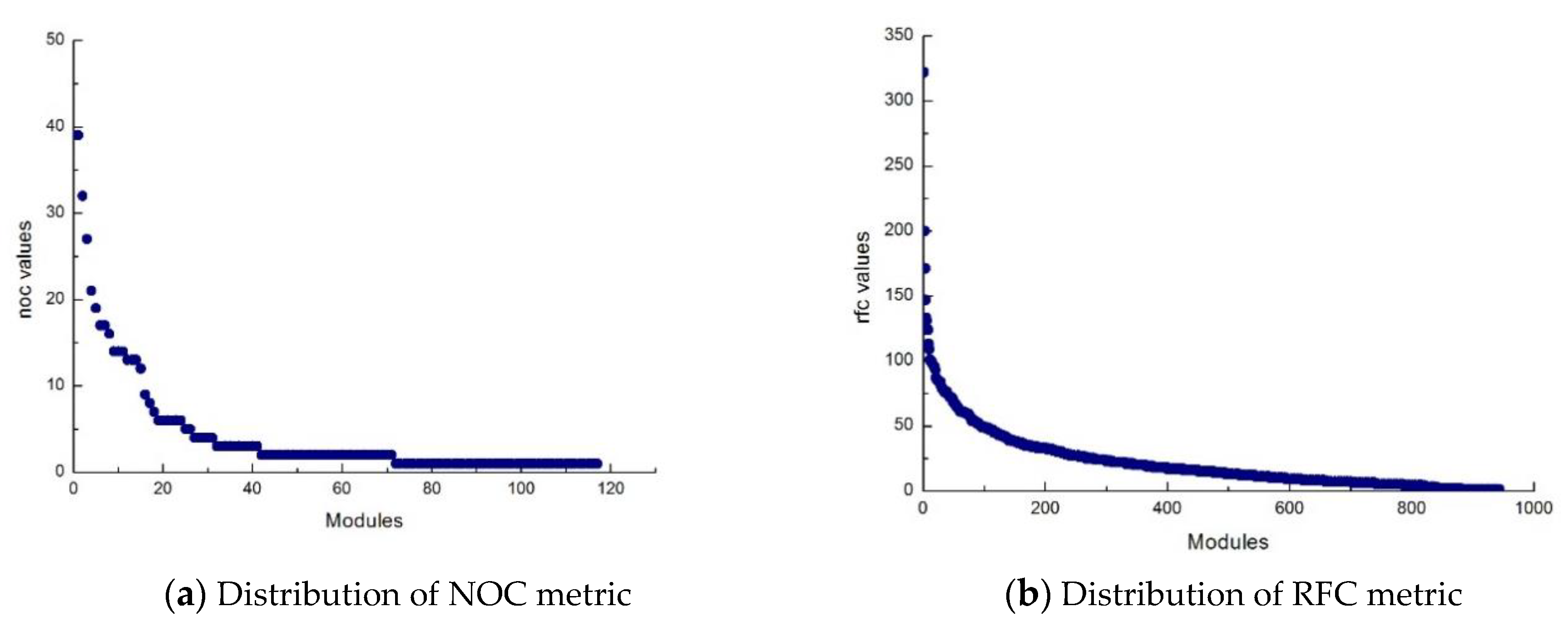
2.1. Correlation and Characteristics

Various power law phenomena can be observed in nature and society, and the study of these phenomena has continued for more than a century. Even now, the power law phenomenon is still a research hotspot in many disciplines. Harvard University linguistics expert George Zipf studied the frequency of English words and found a simple inverse relationship between each word’s frequency and the constant power of its rank in order from large to small. This distribution, known as Zipf’s law, shows that only a few words in English are frequently used and that most words are seldom used [21]. Italian economist Vilfredo Pareto studied the statistical distribution of personal income and found that the income of a few people was much higher than that of the majority. Thus, he put forward the famous 80/20 rule, commonly known as Pareto’s law, in which 20% of the population occupied 80% of the social wealth [22]. Zipf’s law and Pareto’s law are simple power law function patterns. In fact, power law distribution exists in many fields, such as physics, earth and planetary science, computer science, biology, ecology, demography and social science, and economy and finance, and has various manifestations [23,24,25,26,27,28,29,30,31].
Furthermore, Shatnawiand and Althebyan [32] validated the effects power laws have on software metrics interpretations and found that many metrics demonstrate a power law behavior. Furthermore, threshold values with respect to instances were derived from power law function properties. Additionally, Wheeldon and Counsell [33] found that a power law implied that smaller values were commonplace, whereas larger values were extremely rare. Meanwhile, Andersson and Runeson [34] quantitatively analyzed distributions of defects in three different projects and determined through graphical analysis that a small number of instances (20%) were correlated with 63%–70% of prerelease defects.
The general formula of the power law function can be written as:
y = c x γ .
where c and γ are both constants greater than zero.
Logarithms of both sides in Equation (1), ln y and ln x, satisfy a linear relationship. In other words, in the double logarithmic coordinates, the power law function represents a straight line with a negative slope of the power exponent. This linear relationship is the basis for judging whether the random variable in each instance satisfies the power law function [35].
The power law is also a sign of transitioning from steady to chaotic states in the chaotic edge of self-organized critical systems [36]. The power law can be used to predict phases and phase transitions for such systems. Most software defect data have unbalanced distribution characteristics [37], i.e., defect-free instances are more common than defective instances. Many software system defects are concentrated in a small part of the instances, which is characteristic of a power law function.
Figure 1 shows the distributions of the NOC (number of children of a given class in an inheritance tree) and RFC (number of distinct methods invoked by code in a given class) metrics from an example using the Camel1.6 dataset in the Promise database.
As seen in Figure 1, metrics values are distributed in the form of a power law function, which has also been validated by Shatnawi [21]. Therefore, there is a close correlation between the power law function and software system metrics.

2.2. Power Law Function Curvature

Before using power law distribution function to predict software defects, the concept of curvature should be introduced. Curvature refers to the bending degree of a curve [38]. It can be described by the ratio of the angle changed by the curve to the radian changed by the curve. Figure 2 presents a sketch map of power law function curvature. Let M and M be the two points on the curve. If the tangent of the curve at point M and point M and the positive intersection angle of the x-axis are respectively α and α + Δ α . Therefore, when the point changes from M along the curve to M , the angle changes Δ α , and the distance to change this angle is the arc length Δ s = M M . Therefore, curvature is defined by a differential equation to indicate the degree the curve deviates from the straight line. The greater the curvature, the greater the curve’s bending degree and deviation from the straight line. Expression of curvature at point M can be stated as follows.
K = lim Δ s 0 | Δ α Δ s | .
where Δ s tends to zero. The reciprocal of curvature is curve radius, with a larger curve radius yielding a smoother arc. The angle and arc length approaching zero at the same time is the standard curvature definition of a smooth curve with an arbitrary shape.
Obviously, when M’ and M are close enough, the arc length Δ s = M M can be approximately replaced by the chord length MM’, and
lim M M M M M M = 1 .
Therefore, in:
Δ s Δ x = M M Δ x = M M M M M M Δ x = M M M M ( Δ x ) 2 + ( Δ y ) 2 Δ x = M M M M 1 + ( Δ y Δ x ) 2
Let Δ x 0 , the following expression can be obtained by taking the limit:
d s = 1 + y 2 d x
Let the curve equation be y = f ( x ) .
Because t g α = y , so α = a r c t g y , making differential calculation on α = a r c t g y , we will get:
d α = ( a r c t g y ) d x = y 1 + y 2 d x
Therefore, the curvature of a curve can thus be expressed as follows.
k ( x ) = | d α d s | = | y | ( 1 + y 2 ) 3 2
If the metrics power law function is expressed as m ( x ) = α x γ , then:
The first-order derivative of m(x) is m ( x ) = α γ x ( γ + 1 ) ;
The second-order derivative of m(x) is m ( x ) = α γ ( γ + 1 ) x ( γ + 2 ) ;
By finding the first and second derivatives of m(x) and substituting them into Equation (3), the curvature function corresponding to m(x) can be obtained as follows.
k ( x ) = m ( x ) [ 1 + m 2 ( x ) ] 3 2 = α γ ( γ + 1 ) x ( γ + 2 ) [ 1 + α 2 γ 2 x 2 ( γ + 1 ) ] 2 3
As shown in Figure 2, the closer the curve is to the Y axis, the smaller its curvature is, and when the curve is further away from the Y axis, it becomes increasingly curved and thus its curvature increases. At a certain point, the curve begins to essentially parallel to the X axis and the curvature then decreases. This indicates that the power law function curve’s curvature goes from small to large and then from large to small. Thus, a maximum curvature point exists, which may be the transformation point of the metrics from defective to defect-free. In other words, the maximum curvature point of a power law function can be taken as the demarcation point between defective and defect-free instances. Therefore, if this transition point is calculated, it can be used as a threshold value for estimating whether the entity in the metric has defects. Consequently, the transformation point divides the metrics into two parts, defective and non-defective.
A curve’s maximum curvature point should be a point with a first-order derivative of zero for the curvature function k ( x ) . The first-order derivative of k ( x ) can be obtained as follows.
k ( x ) = α γ ( γ + 1 ) ( γ + 2 ) x ( γ + 3 ) [ 1 + α 2 γ 2 x 2 ( γ + 1 ) ] 3 2 + 3 α 3 γ 3 ( γ + 1 ) 2 x ( 3 γ + 5 ) [ 1 + α 2 γ 2 x 2 ( γ + 1 ) ] 1 2 [ 1 + α 2 γ 2 x 2 ( γ + 1 ) ] 3
Let k ( x ) = 0 , when [ 1 + α 2 γ 2 x 2 ( γ + 1 ) ] 3 0 ,we have:
α γ ( γ + 1 ) ( γ + 2 ) x ( γ + 3 ) [ 1 + α 2 γ 2 x 2 ( γ + 1 ) ] 3 2 + 3 α 3 γ 3 ( γ + 1 ) 2 x ( 3 γ + 5 ) [ 1 + α 2 γ 2 x 2 ( γ + 1 ) ] 1 2 = 0
when x 0 , dividing both sides by α γ ( γ + 1 ) x ( γ + 3 ) [ 1 + α 2 γ 2 x 2 ( γ + 1 ) ] 1 2 we will get:
( γ + 2 ) [ 1 + α 2 γ 2 x 2 ( γ + 1 ) ] + 3 α 2 γ 2 ( γ + 1 ) x 2 ( γ + 1 ) = 0
Therefore, the derivative of the curvature function of a power law function is obtained and made to be zero and can be obtained as follows:
x 2 ( γ + 1 ) = α 2 γ 2 ( 2 γ + 1 ) γ + 2
That is, the X coordinate of the maximum curvature point of power function is:
x = α 2 γ 2 ( 2 γ + 1 ) γ + 2 2 ( γ + 1 ) = [ α 2 γ 2 ( 2 γ + 1 ) γ + 2 ] 1 2 ( γ + 1 )
Consequently, the transformation point in the corresponding metrics can be obtained as:
m ( x ) = α x γ
That is to say, entities within the metrics can be classified into a defective tendency group when parameter values are greater than m ( x ) , because for most metrics, software entities containing defects generally have larger values than those without defects [39,40,41,42]. In contrast, other entities are classified into a defect-free tendency group when parameter values are less than m ( x ) .
Taking as an example, for the function of y = x 2 , the image of this function can be seen in Figure 3. By Equation (13), it can be calculated that the maximum curvature point of the power function at x-axis is x = 1.31 , the y value can be calculated as 0.5848. Therefore, we can obtain the transformation point as shown in Figure 3.
Therefore, this study chooses the value m ( x ) in the maximal curvature point as the threshold value for evaluating whether each entity in the metric is defect-free or defective.

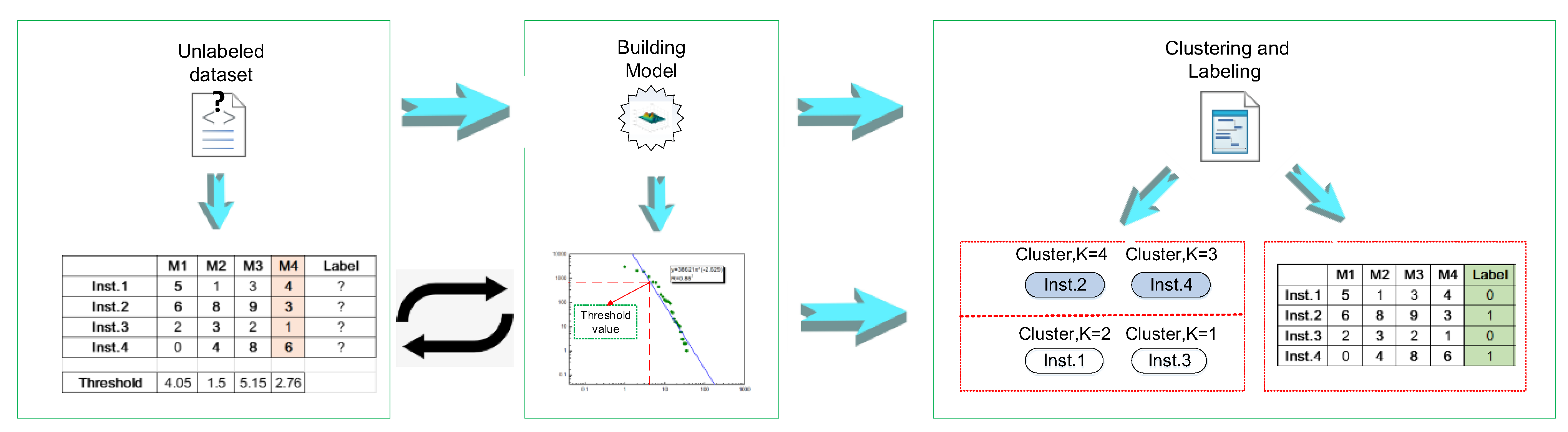
2.3. Approach for Software Defect Prediction Based on Power Law Function

In this section, we present the approach for detecting software defects based on the power law function. The general algorithm of the proposed model is expressed in Algorithm 1:
Algorithm 1. Software defect prediction based on power-law function
Input
D ← Original unlabeled datasets
Inst. ← Instances in datasets
M ← Each metric in dataset D
MV ← Each value of the metric in dataset D
1  for M in All M do
2  for i = 1 to number of M do
3  Building power-law function for each M
4  According to Equation (14),
  compute transformation value in maximal curvature point T
5   if MVi. Insti > T
6    MVi. Insti is higher value, MVi. Insti = 1
7   else
8    MVi. Insti is normal value, MVi. Insti = 0
9   end if
10  end for
11  for each Insti in Inst.
12  Calculate the total number K of each Insti in the D with MVi. Insti = 1
13  Sort values of K, clustering into two groups, a top half and a bottom half.
14  for i = 1 to number of Inst. do
15  compare each K value in Inst.
16   if K values in top half
17    Inst.i is defect-proneness
18   else
19    Inst.i is defect-free tendency
20   end if
21  end for
Output
Dataset with defect label
Figure 4 shows the overall process of this approach. The kernel of our approach is to use the power law function to describe the metrics distribution and set the transformation value of the maximal curvature point as the threshold value to label the metrics.
The process is stated in detail as follows.
1. Establish power law functions for each metric
A power law function is used to establish the linear regression model for each metric by sorting parameter values from large to small and numbering corresponding software modules from 1 to n (n is the number of software instances). This is a straight line in the double logarithmic coordinate system.
2. Calculate each metric’s threshold value
The threshold value is the critical value, which can be used to judge whether a software system fault exists under the metrics. Therefore, Equation (13) is used to calculate the position of the maximum curvature value of the obtained power law function. The value obtained from Equation (14) at this position is the approximate boundary between the defective and defect-free metrics.
3. Identify the defective tendency of metrics
Identifying the defective tendency of instances under a certain metric in software defect prediction is generally based on the assumption that a defective instance’s parameter value tends to be higher than that of non-defective instances [39,40,41,42]. Therefore, entities with parameters larger than the threshold value are identified as defective and set as 1. In contrast, other entities are identified as defect-free and set as 0.
4. Calculate the total number of entities in the metrics with a value of 1
5. Label the instances by clustering
Instances are clustered into a top half and a bottom half, with instances in the top half labeled as defective and others labeled as defect-free.
Based on the proposed approach, we can predict software defects without relying on labeled datasets. The following case studies and comparisons have been conducted to validate the feasibility of the new approach.

3. Experimental

3.1. Case Study

To conduct a case study, we selected the public Camel1.6 dataset. The Camel1.6 dataset has 965 instances, of which 188 were defective and 777 were defect-free [43]. Defective instances accounted for 19.48% of the total instances. Each instance had 20 metric parameters and the label of each instance was removed in advance. Followingly, the power law function was established for each metric and correlation coefficients were calculated.
The power law function, correlation coefficient, and transformation value in the maximal curvature point are shown in Table 1.
Boldface indicates that the correlation coefficients were smaller than 0.3, which didn’t exhibit the characteristics of power law function.
Most of the metric parameters can be described well with power law functions. The correlation coefficients were mostly larger than 0.7, indicating that the power law function effectively described the metrics parameters distribution. Although two metrics were not well described by the power law functions, the ratio was relatively small. Figure 5 shows comparisons between the actual metrics data scatter and corresponding power law functions. Good consistencies were obtained for different metrics.
Based on the calculated transformation values in each power law function’s maximal curvature point, each entity with a value larger than the transformation value was identified as defective and set as 1 and others were identified as defect-free and set as 0. Following this, the total number of defective entities in each instance was calculated and listed. Finally, instances were labeled by clustering into two groups, a top half and a bottom half. Therefore, the instances in the top half of the clusters were labeled as defective and the others were labeled as defect-free. The number of defects predicted by the proposed approach was 94 and the number of actual defects was 188. Therefore, the precision of the proposed approach with respect to the Camel1.6 dataset was 0.276.

3.2. Performance Evaluation

Performance evaluations of software defect prediction are based on the confusion matrix, as shown in Table 2, which includes the measures of precision, recall, and F-measure [44].
True positive (TP) is the number of defective entities predicted as defective.
False negative (FN) is the number of defective entities predicted as defect-free.
False positive (FP) is the number of defect-free entities predicted as defective.
True negative (TN) is the number of defect-free entities predicted as defect-free.
In this study, predictive performance measures are computed as follows:
{ P r e c i s i o n = T P T P + F N R e c a l l = T P T P + F P F m e a s u r e = 2 × R e c a l l × P r e c i s i o n R e c a l l + P r e c i s i o n
Precision represents the proportion of defective entities to all entities correctly predicted as defective.
Recall represents the proportion of defective entities to all entities that are actually defective.
F-measure is the harmonic average of recall and accuracy, with higher F-measure values corresponding to better prediction performance.

3.3. Comparative Experiment

To verify the performance of the proposed software defect prediction approach, we selected four classic algorithms used for defect prediction with unlabeled datasets: k-means [16,17], CLA and CLAMI (Clustering and labeling Approach based on Matric Instances) [4], and x-means [18]. These traditional methods are based on classical data clustering method, such as k-means, x-means and so on. We compared the proposed approach with these algorithms on twelve randomly selected public datasets [43,44,45]. These public datasets are produced from real software systems, with different sizes and types, which can be utilized as a representation for different software systems.
Details of datasets used in the comparative experiment (Section 3.3) are shown in Table 3. The selected algorithms were common unsupervised software defect prediction algorithms.
Table 4, Table 5 and Table 6 show comparisons of precision, recall, and F-measure results between the proposed approach and other methods in the comparative experiment. The highest values of each dataset are highlighted in bold.
The proposed approach was generally superior to other traditional methods in terms of precision, recall, and the F-measure. Although the average precision value obtained by the proposed approach was not the best, the proposed approach performed the best in 6 of 12 datasets in terms of precision, giving it the largest number of optimal results among the tested methods. Furthermore, the average precision values of the proposed approach and the k-means algorithm were relatively similar.
For the recall value, the proposed approach’s advantage was much more apparent. It performed the best in 10 of the 12 datasets and had an average value of 0.790, which was the highest among the tested methods. It was obvious that the proposed approach performed significantly better than traditional defect prediction models on almost all datasets. At the same time, some researchers have indicated that prediction models with low precision and high recall were more useful in many industrial situations [46]. The proposed approach obtained a better recall value than the precision value and thus would perform better in these areas.
For the F-measure value, the proposed approach performed the best in 7 of the 12 datasets and had the largest average value of 0.501 among the tested methods. It was clear that the proposed approach obtained the best F-measure value and thus demonstrated the proposed approach’s effectiveness at software defect prediction with unlabeled datasets.
Therefore, based on these public datasets, it can be seen that the proposed approach obtains the best prediction results among the tested five algorithms. Nevertheless, considering the limitation of data timeliness and scale, these datasets cannot totally represent the real software defects and new defects. When utilized in real software systems, the proposed approach can be further validated.

4. Complexity Analysis

Authors should discuss the results and how they can be interpreted in perspective of previous studies and of the working hypotheses. The findings and their implications should be discussed in the broadest context possible. Future research directions may also be highlighted.
Algorithm complexities of the other algorithms tested in this study are shown in Table 7. The complexity of k-means, CLA, and CLAMI were obtained from references [4,17]. The proposed approach has a relatively lower complexity than the other algorithms, indicating a low cost in software defect predictions. Therefore, from the perspective of algorithm complexity, our proposed approach possesses some advantages over the other tested algorithms to some extent.

5. Conclusions

In this study, we proposed a novel approach that adopted characteristics of the power law function for software defect prediction. The kernel of our approach was using the power law function to describe metrics distributions and set the transformation values in the maximal curvature point of each power law function curve as the threshold value for labeling metrics. In our empirical studies, we found that the proposed approach performed significantly better than other commonly used four algorithms across all evaluated twelve terms. The average values of recall and F-measure were improved by over 14.3% and 6.0%, respectively. Furthermore, the proposed approach had a complexity of O ( 2 n ) , which was the lowest among the tested five algorithms. Therefore, we demonstrated that our proposed approach is feasible and highly efficient at defect prediction with unlabeled datasets.
In summary, the proposed approach offers a viable choice for software defect prediction on unlabeled datasets. However, similar to any other method, there are some issues to handle in future work. The precision of the prediction should be analyzed in-depth and improved in the future. At the same time, future work should attempt to use the proposed approach to rank predictions.

Author Contributions

Conceptualization, methodology, writing—original draft preparation and software, J.R. Project administration, funding acquisition, F.L. All authors have read and agreed to the published version of the manuscript.

Funding

This work was supported by the Fundamental Research Funds for the Central Universities (Grant No. 2019JBM026).

Conflicts of Interest

The authors declare no conflict of interest.

Appendix A

The metrics and their descriptions for dataset Camel1.6 utilized in case study.
MetricsDescription
wmcWeighted methods per class
ditThe maximum distance from a given class to the root of an inheritance tree
nocNumber of children of a given class in an inheritance tree
cboNumber of classes that are coupled to a given class
rfcNumber of distinct methods invoked by code in a given class
lcomNumber of method pairs in a class that do not share
access to any class attributes
caAfferent coupling, which measures the number of classes
that depend on a given class
ceEfferent coupling, which measures the number of classes
that a given class depends on
npmNumber of public methods in a given class
lcom3Another type of the lcom metric proposed by
Henderson–Sellers
locNumber of lines of code in a given class
damThe ratio of the number of private/protected attributes
to the total number of attributes in a given class
moaNumber of attributes in a given class that are of
user-defined types
mfaNumber of methods inherited by a given class divided
by the total number of methods that can be accessed by
the member methods of the given class
camThe ratio of the sum of the number of different parameter
types of every method in a given class to the product of
the number of methods in the given class and the number
of different method parameter types in the whole class
icNumber of parent classes that a given class is coupled to
cbmTotal number of new or overwritten methods that all
inherited methods in a given class are coupled to
amcThe average size of methods in a given class
max_ccThe maximum McCabe’s cyclomatic complexity (CC)
score of methods in a given class
avg_ccThe arithmetic mean of McCabe’s cyclomatic complexity (CC) scores of methods in a given class

References

  1. Ekanayake, J.; Tappolet, J.; Gall, H.C.; Bernstein, A. Tracking concept drift of software projects using defect prediction quality. In Proceedings of the 6th International Working Conference on Mining Software Repositories, MSR 2009 (Co-located with ICSE), Vancouver, BC, Canada, 16–17 May 2009. [Google Scholar] [CrossRef] [Green Version]
  2. Li, L.; Lessmann, S.; Baesens, B. Evaluating software defect prediction performance: An Updated Benchmarking Study. SSRN Electron. J. 2019, arXiv:1901.01726. [Google Scholar] [CrossRef] [Green Version]
  3. Balogun, A.O.; Basri, S.; Abdulkadir, S.J.; Hashim, A.S. Performance Analysis of Feature Selection Methods in Software Defect Prediction: A Search Method Approach. Appl. Sci. 2019, 9, 2764. [Google Scholar] [CrossRef] [Green Version]
  4. Nam, J.; Kim, S. CLAMI: Defect prediction on unlabeled datasets (T). In Proceedings of the 30th IEEE/ACM International Conference on Automated Software Engineering (ASE), Lincoln, NE, USA, 9–13 November 2015; pp. 452–463. [Google Scholar] [CrossRef]
  5. Zimmermann, T.; Nagappan, N.; Gall, H.; Giger, E.; Murphy, B. Cross-project defect prediction: A large scale experiment on data vs. domain vs. process. In Proceedings of the Joint Meeting of the European Software Engineering Conference on the Foundations of Software Engineering, Amsterdam, The Netherland, 24–28 August 2009; pp. 91–100. [Google Scholar]
  6. Chen, X.; Wang, L.P.; Gu, Q.; Wang, Z.; Ni, C.; Liu, W.S.; Wang, Q.P. A survey on cross-project software defect prediction methods. Chin. J. Comput. 2018, 41, 254–274. [Google Scholar] [CrossRef]
  7. Qiu, S.; Lu, L.; Jiang, S.; Guo, Y. An investigation of imbalanced ensemble learning methods for cross-project defect prediction. Int. J. Pattern Recogn. 2019. [Google Scholar] [CrossRef]
  8. Mao, F.G.; Li, B.W.; Shen, B.J. Cross-project software defect prediction based on instance transfer. J. Comput. Sci. Tech.-Ch. 2016, 10, 43–55. [Google Scholar] [CrossRef]
  9. Jureczko, M.; Nguyen, N.T.; Szymczyk, M.; Unold, O. Towards implementing defect prediction in the software development process. J. Intell. Fuzzy Syst. 2019, in press. [Google Scholar] [CrossRef]
  10. Malhotra, R.; Khanna, M. Prediction of change prone classes using evolution-based and object-oriented metrics. J. Intell. Fuzzy Syst. 2018, 34, 1755–1766. [Google Scholar] [CrossRef]
  11. Catal, C.U.; Sevim, U.; Diri, B. Clustering and metrics thresholds based software fault prediction of unlabeled program modules. In Proceedings of the 6th International Conference on Information Technology: New Generations, Las Vegas, NV, USA, 27–29 April 2009; pp. 199–204. [Google Scholar] [CrossRef]
  12. Catal, C.; Sevim, U.; Diri, B. Software fault prediction of unlabeled program modules. Lect. Notes Eng. Comput. Sci. 2009, 2176, 199–204. [Google Scholar] [CrossRef]
  13. Abaei, G.; Rezaei, Z.; Selamat, A. Fault prediction by utilizing self-organizing map and threshold. In Proceedings of the 2013 IEEE International Conference on control system, Mindeb, Malaysia, 29 November–1 December 2013; pp. 465–470. [Google Scholar] [CrossRef]
  14. Yang, B.; Yin, Q.; Xu, S.; Guo, P. Software quality prediction using affinity propagation algorithm. In Proceedings of the 2008 IEEE International Joint Conference on Neural Networks (IEEE World Congress on Computational Intelligence), Hong Kong, China, 1–8 June 2008; pp. 2161–4393. [Google Scholar] [CrossRef]
  15. Bishnu, P.S.; Bhattacherjee, V. Application of k-medoids with kd-tree for software fault prediction. ACM Sigsoft Softw. Eng. Notes 2011, 36, 1–6. [Google Scholar] [CrossRef]
  16. Bishnu, P.S.; Bhattacherjee, V. Software fault prediction using quad tree-based k-means clustering algorithm. IEEE Trans. Knowl. Data Eng. 2012, 24, 1146–1150. [Google Scholar] [CrossRef]
  17. Zhong, S.; Khoshgoftaar, T.M.; Seliya, N. Unsupervised learning for expert-based software quality estimation. IEEE Int. Symp. High Assur Syst. Eng. 2004, 149–155. [Google Scholar] [CrossRef]
  18. Park, M.; Hong, E. Software fault prediction model using clustering algorithms determining the number of clusters automatically. Int. J. Softw. Eng. Appl. 2014, 8, 199–204. [Google Scholar]
  19. Lu, Z.F. Software Defect Prediction Research for Unlabeled Datasets. Master’s Thesis, Chongqing University, Chongqing, China, 2016. [Google Scholar]
  20. Newman, M.E.J. Power laws, Pareto distributions and Zipf’s law. Contemp. Phys. 2005, 46, 323–351. [Google Scholar] [CrossRef] [Green Version]
  21. Adamic, L.A.; Huberman, B.A.; Barabási, A.L.; Albert, R.; Jeong, H.; Bianconi, G. Power-law distribution of the world wide web. Science 2000, 287, 2115. [Google Scholar] [CrossRef] [Green Version]
  22. Levy, M.; Solomon, S. New evidence for the power-law distribution of wealth. Physica A 1997, 242, 90–94. [Google Scholar] [CrossRef]
  23. Pareto, V. The new theories of economics. J. Political Econ. 1897, 5, 485–502. [Google Scholar] [CrossRef]
  24. Gabriel, S.B.; Feynman, J. Power-law distribution for solar energetic proton events. Sol. Phys. 1996, 165, 337–346. [Google Scholar] [CrossRef]
  25. Zhang, Y.L.; Han, T.L.; Lang, B.H.; Li, Y.; Lai, F.W. Detection and extraction of shockwave signal in noisy environments. J. Intell. Fuzzy Syst. 2019, in press. [Google Scholar] [CrossRef]
  26. Bredenoord, A.J.; Smout, A.J.P.M. Oesophageal pH has a power-law distribution in control and gastro-oesophageal reflux disease subjects. Alimen. Pharm. Ther. 2005, 21, 917. [Google Scholar] [CrossRef]
  27. Zhang, S.Z.; Wei, Y.D.; Liang, X. Research on power-law distribution and identification of Kinship in mobile social network. J. Chin. Inf. Process. 2018, 32, 14–122. [Google Scholar]
  28. Jiang, B.; Yang, C.; Wang, L.; Li, R.G. Mining multiplex power-law distributions and retweeting patterns on twitter. J. Intell. Fuzzy Syst. 2016, 31, 1009–1016. [Google Scholar] [CrossRef]
  29. Louridas, P.; Spinellis, D.; Vlachos, V. Power laws in software. ACM Trans. on Softw. Eng. Methodol. 2008, 18, 1–26. [Google Scholar] [CrossRef]
  30. Concas, G.; Marchesi, M.; Pinna, S.; Serra, N. Power-laws in a large object-oriented software system. IEEE Trans. Softw. Eng. 2007, 33, 687–708. [Google Scholar] [CrossRef]
  31. Hatton, L. Power-law distributions of component size in general software systems. IEEE Trans. Softw. Eng. 2009, 35, 566–572. [Google Scholar] [CrossRef]
  32. Shatnawi, R.; Althebyan, Q. An empirical study of the effect of power law distribution on the interpretation of OO metrics. Isrn Softw. Eng. 2013, 1–18. [Google Scholar] [CrossRef] [Green Version]
  33. Wheeldon, R.; Counsell, S. Power law distributions in class relationships. In Proceedings of the IEEE International Workshop on Source Code Analysis and Manipulation, Amsterdam, The Netherlands, 26–27 September 2003; pp. 45–54. [Google Scholar] [CrossRef] [Green Version]
  34. Andersson, C.; Runeson, P. A replicated quantitative analysis of fault distributions in complex software systems. IEEE Trans. Softw. Eng. 2007, 33, 273–286. [Google Scholar] [CrossRef]
  35. Mitzenmacher, M. A brief history of generative models for power law and lognormal distributions. Internet Mathematics. 2004, 1, 226–251. [Google Scholar] [CrossRef] [Green Version]
  36. Clauset, A.; Shalizi, C.R.; Newman, M.E.J. Power-law distributions in empirical data. Siam Rev. 2009, 51, 661–703. [Google Scholar] [CrossRef] [Green Version]
  37. Ma, Y.; Pan, W.W.; Zhu, S.Z.; Yin, H.Y. An improved semi-supervised learning method for software defect prediction. J. Intell. Fuzzy Syst. 2014, 27, 2473–2480. [Google Scholar] [CrossRef]
  38. Xiao, X.H.; Yu, M. Advanced Mathematics, 5th ed.; Higher Education Press: Beijing, China, 2006; pp. 167–170. [Google Scholar]
  39. Zhang, F.; Zheng, Q.; Zou, Y.; Hassan, A.E. Cross-project defect prediction using a connectivity-based unsupervised classifier. In Proceedings of the 2016 IEEE/ACM 38th International Conference on Software Engineering (ICSE), Austin, TX, USA, 14–22 May 2016; pp. 309–320. [Google Scholar] [CrossRef]
  40. Ambros, M.D.; Lanza, M.; Robbes, R. Evaluating defect prediction approaches: A benchmark and an extensive comparison. Empir. Softw. Eng. 2012, 17, 531–577. [Google Scholar] [CrossRef]
  41. Gaffney, J.E. Estimating the number of faults in code. IEEE Trans. Softw. Eng. 1984, 10, 459–464. [Google Scholar] [CrossRef]
  42. Hassan, A.E. Predicting faults using the complexity of code changes. In Proceeding of the 2009 IEEE 31st International Conference on Software Engineering, Vancouver, BC, Canada, 16–24 May 2009; pp. 78–88. [Google Scholar] [CrossRef]
  43. Jureczko, M.; Madeyski, L. Towards identifying software project clusters with regard to defect prediction. In Proceedings of the 6th International Conference on Predictive Models in Software Engineering, Promise 2010, Timisoara, Romania, 12–13 September 2010. [Google Scholar] [CrossRef] [Green Version]
  44. Jiang, Y.; Cukic, B.; Ma, Y. Techniques for evaluating fault prediction models. Empir. Softw. Eng. 2008, 13, 561–595. [Google Scholar] [CrossRef]
  45. Wu, R.; Zhang, H.; Kim, S.; Cheung, S.C. ReLink: Recovering links between bugs and changes. In Proceedings of the 19th ACM SIGSOFT Symposium and the 13th European conference on Foundations of Software Engineering, Szeged, Hungary, 5–9 September 2011; pp. 15–25. [Google Scholar] [CrossRef]
  46. Menzies, T.; Dekhtyar, A.; Distefano, J.; Greenwald, J. Problems with precision: A response to comments on data mining static code attributes to learn defect predictors. IEEE Trans. Softw. Eng. 2007, 33, 637–640. [Google Scholar] [CrossRef] [Green Version]
Figure 1. Distributions of metrics values of number of children of a given class in an inheritance tree (NOC) and number of distinct methods invoked by code in a given class (RFC) in the Camel1.6 dataset.
Applsci 10 01892 g001
Figure 2. Power law function curvature.
Applsci 10 01892 g002
Figure 3. The image of y = x 2 and its transformation point with the maximal curvature.
Applsci 10 01892 g003
Figure 4. The overall process of the proposed unsupervised approach in software defect prediction.
Applsci 10 01892 g004
Figure 5. Power law functions with respect to different metrics. (a) wmc: weighted methods per class; (b) noc: number of children of a given class in an inheritance tree; (c) cbo: number of classes that are coupled to a given class; (d) lcom: number of method pairs in a class that do not share access to any class attributes; (e) ca: afferent coupling, which measures the number of classes that depend on a given class; (f) npm: number of public methods in a given class.
Applsci 10 01892 g005
Table 1. Power law function, correlation coefficient, and transformation value in the maximal curvature point. The metrics and their descriptions can be seen in Appendix A.
MetricsPower Law FunctionCorrelation CoefficientTransformation Value
wmc1013.8 x 0.892 0.846641.31
dit34.841 x 0.516 0.790913.51
noc110.68 x 1.012 0.947910.30
cbo915.03 x 0.83 0.85445.82
rfc4273 x 0.996 0.724766.07
lcom34730 x 1.816 0.899458.94
ca834.42 x 1.015 0.968427.93
ce554.53 x 0.821 0.776535.63
npm994.19 x 0.934 0.875236.86
lcom319.53 x 0.518 0.55189.19
loc129509 x 1.355 0.6554120.88
dam1.3429 x 0.063 0.04341.56
moa23.007 x 0.564 0.89059.44
mfa2.327 x 0.219 0.29772.73
cam6.9114 x 0.473 0.69284.91
ic3.5344 x 0.241 0.71843.80
cbm68.343 x 0.757 0.930812.73
amc463.68 x 0.671 0.886947.49
max_cc108.78 x 0.713 0.918718.20
avg_cc11.099 x 0.431 0.86487.21
Table 2. Confusion matrix.
ActualPredicted
TrueFalse
TrueTP (true positive)FN (false negative)
FalseFP (false positive)TN (true negative)
Table 3. Overview of experimental datasets.
GroupDataset# of instances# of Metrics
AllBuggy (%)
PromiseCamel1.6965188 (19.48%)20
Forrest-0.8322 (6.25%)
Synapse-1.015716 (10.19%)
Berek4316 (37.21%)
Intercafe274 (14.81%)
Termo4213 (30.95%)
Pbean25110 (19.61%)
SoftLabar11219 (7.44%)29
ar410720 (18.69%)
ar5368 (22.22%)
ReLinkApache19498 (50.52%)26
Safe5622 (39.29%)
Table 4. Comparisons of precision results between the proposed approach and other methods.
DatasetsMethods
K-MeansCLACLAMIX-MeansPower Law Function Approach
Camel1.60.1460.2470.2470.2560.276
Forrest-0.80.0400.0760.0700.0710.125
Synapse-1.00.0330.1890.0290.0340.194
Berek1.0000.6360.6320.3850.778
Intercafe-0.2300.2300.1110.231
Termo0.4000.4670.5000.4210.571
Pbeans20.2760.3750.3080.2760.364
ar10.1380.1150.1070.2500.119
ar40.3330.3400.3070.6000.333
ar50.6360.4700.4440.6300.444
Apache0.7140.7260.7370.6250.737
Safe0.7330.6400.6300.6500.607
Average0.4040.3760.3530.3590.398
Boldface typeface indicates the highest value of each dataset.
Table 5. Comparisons of recall results between the proposed approach and other methods.
DatasetsMethods
K-MeansCLACLAMIX-MeansPower Law Function Approach
Camel1.60.2820.5210.6220.3350.500
Forrest-0.80.5000.5000.5000.5001.000
Synapse-1.00.0630.4380.0630.0630.875
Berek0.2500.8750.7500.3130.875
Intercafe--0.7500.7500.2500.750
Termo0.6150.5380.6920.6150.615
Pbeans20.8000.6000.4000.8000.800
ar10.6670.6670.6670.6000.778
ar40.8000.8000.8000.1500.800
ar50.8751.0001.0000.9001.000
Apache0.2760.7040.7140.4590.714
Safe0.5000.7270.7730.5910.773
Average0.5120.6770.6440.4650.790
Boldface typeface indicates the highest value of each dataset.
Table 6. Comparisons of F-measure results between the proposed approach and other methods.
DatasetsMethods
K-MeansCLACLAMIX-MeansPower law Function Approach
Camel1.60.1920.3360.3530.2900.355
Forrest-0.80.0740.1330.1250.1250.222
Synapse-1.00.0430.2640.0400.0440.318
Berek0.4000.7370.6860.3450.824
Intercafe-0.3750.3530.1540.353
Termo0.4850.5000.5810.5000.593
Pbeans20.4100.4620.3480.4100.500
ar10.2290.1970.1850.3530.206
ar40.4710.4780.4440.2400.471
ar50.7370.6400.6150.7400.615
Apache0.4090.7150.7250.5290.725
Safe0.5950.6810.6940.6190.680
Average0.3850.4710.4360.3690.501
Boldface typeface indicates the highest value of each dataset.
Table 7. Complexity of the tested algorithms.
MethodK-MeansCLACLAMIX-meansPower-Law Function Approach
Complexity O ( n k m ) O ( 2 n + n 2 ) O ( 3 n + n 2 ) - O ( 2 n )

