Use of Deep Multi-Target Prediction to Identify Learning Styles

Featured Application

Our results can be applied to identifying of students’ learning style providing adaptation to e-learning systems.

Abstract

It is possible to classify students according to the manner they recognize, process, and store information. This classification should be considered when developing adaptive e-learning systems. It also creates a comprehension of the different styles students demonstrate while in the process of learning, which can help adaptive e-learning systems offer advice and instructions to students, teachers, administrators, and parents in order to optimize students’ learning processes. Moreover, e-learning systems using computational and statistical algorithms to analyze students’ learning may offer the opportunity to complement traditional learning evaluation methods with new ones based on analytical intelligence. In this work, we propose a method based on deep multi-target prediction algorithm using Felder–Silverman learning styles model to improve students’ learning evaluation using feature selection, learning styles models, and multiple target classification. As a result, we present a set of features and a model based on an artificial neural network to investigate the possibility of improving the accuracy of automatic learning styles identification. The obtained results show that learning styles allow adaptive e-learning systems to improve the learning processes of students.

1. Introduction

According to Willingham [1], people are normally curious but are not naturally acceptable masterminds; unless cognitive conditions are adequate, humans abstain from reasoning. This behavior is attributed to three properties. To begin with, reasoning is used with moderation; human’s visual system is proficient to instantly take in a complex scene, although it is not inclined to instantly solve a puzzle. Additionally, reasoning is tiresome because it requires focus and concentration. Finally, because we ordinarily make mistakes, reasoning is uncertain. In spite of these aspects, humans like to think. Solving problems produces pleasure because there is an overlap between the brain’s areas and chemicals that are important in learning and those related to the brain’s natural reward system [1]. Thus, adjusting a student’s cognitive style might help to improve the student’s reasoning capacity.

Moreover, according to Felder and Silverman [2], learning styles (a part of cognitive styles) describe students’ preferences on how some subject is presented, how to work with that subject matter, and how to internalize (acquire, process, and store) information [2]. According to Willingham [1], students may have diverse preferences on how to learn. Thus, knowing a student’s learning style can help in finding the most suitable way to improve the learning process. There are some studies which show that learning styles allow adaptive e-learning systems to improve the learning processes of students [3,4,5,6,7].

We characterize learning as the procedure through which information is encoded and stored in the long-term memory. For instance, customizing content to the learning styles of students is seen as useful to learning in different ways, for example, improving fulfillment, increasing learning results, and decreasing learning time [3]. Several research works in learning systems proposed that students’ learning improved when the instructor’s teaching style matched the learning style of the students [5].

According to Bernard et al. [5], there are several methods to classify learning styles. One of the most known is the Felder–Silverman learning styles model (FSLSM). This model proposes four dimensions to classify learning styles, with each dimension classified in an interval ranging from 0 to 11. The first dimension of this model is active/reflective, which determines if someone prefers first experimenting with some subject and then reasoning about it (active) or reasoning first and then experimenting on the subject (reflective). The second dimension is sensing/intuitive, which determines if someone prefers touching things to learn (sensing) or observing things to induce information (intuitive). The third dimension, visual/verbal, determines if someone prefers to see charts, tables, and figures (visual) instead of reading or listening to texts (verbal), or the contrary. Finally, the sequential/global dimension determines if someone prefers to get information in a successive manner, learning step-by-step (sequential), or to get an outline of the information first and go into detail afterwards, without a predefined sequence (global).

According to Willingham [1], the prediction of any learning styles theory is that a particular teaching method might be good for some students but not so good for others. Therefore, it is possible to take advantage of different types of learning. It is important to understand the difference between learning ability and learning style. Learning ability is the capacity for or success in certain types of thought (math, for example). In contrast to ability, learning style is the tendency to think in a particular way, for example, thinking sequentially or holistically, which is independent of context [1]. There is an enormous contrast between the popularity of learning styles in education and evidence of their usefulness. According to Pashler [4], the reasonable utility of using learning styles to improve student learning still needs to be demonstrated. However, in their study, Kolb and Kolb [6] examined recent research advancements in experimental learning in higher education and analyzed how it can improve students’ learning. In their studies they concluded that learning styles can be based on research and clinical observation of learning styles’ score patterns and applied throughout the educational environment through an institutional development program.

As indicated by Willingham [1], psychologists have made a few approaches to test this learning proposition, leading to some hypotheses. First, learning style is considered as stable within an individual. In other words, if a student has a particular learning style, that style ought to be a stable part of that student’s cognitive makeup. Second, learning style ought to be consequential; therefore, using a specific learning style should have implications on the outcomes of the student’s learning. Thus, learning styles theory must have the following three features: (1) a specific learning style should be a stable characteristic of a person; (2) individuals with different styles should think and learn differently; and (3) individuals with different styles do not, on average, differ in their ability. Traditionally, learning styles are mainly measured through surveys and questionnaires, where students are asked to self-evaluate their own behaviors. However, this approach presents some problems. First, external interference can disturb the results during its application. Second, the outcomes are influenced by the quality of the survey or questionnaire. Finally, different students may interpret questions in different ways [5].

According to Bernard et al. [4], the characterization of learning styles is a problem that deals with many descriptors and many outputs. The descriptors may arise from many sources, such as logs, questionnaires, and databases. Moreover, the descriptors are usually associated with learning objects, such as forums, contents, outlines, quizzes, self-assignments, examples, and other types of resources. The outputs are used to permit the comprehension of learning style resulting from a combination of descriptors, which may indicate whether a student can be classified as active/reflective, sensing/intuitive, visual/verbal, or sequential/global, based on his/her approach to recognize, process, and store information. This problem is relevant because it is the first step to understand the cognitive condition to improve learning using e-learning systems [5].

In this context, our research aims to investigate the use of computational intelligence (CI) algorithms to analyze and improve the accuracy of autonomic approaches to identify learning style. Our hypothesis is that if the learning style can be correctly identified using CI then the student’s learning preference may also be predicted. Thus, we conducted this research to identify features that may represent a student’s learning style based on massive information (big data) collected in a massive open online course (MOOC) environment and use these features to classify these learning styles. We also investigate whether a theory of learning style might be more suited to classification than others. Finally, we investigate algorithms to overcome limitations found in contemporary works.

This paper is organized as follows: This first section presents basic considerations and justifications for this work and defines its main objectives. Section 2 presents an overall review of the key topics treated here and the main definitions upon which this work is based. Section 3 presents the main concepts behind learning styles classification and describes the proposed model. Section 3 also presents the data structures used to characterize the subjects, along with their materials and methods. Section 4 presents the results obtained from the data analysis and specifies recommendations to stakeholders. In the last section, conclusions and future developments are presented.

2. Related Work and Concepts

According to Truong [7] and Normadhi [3], researchers have been searching for mechanisms to automatically detect student’s learning styles based on different models. The process of automatic learning style detection can be divided into three subproblems: (a) select a suitable learning model, (b) select the descriptors and targets to represent a student’s online behavior (in a MOOC), and (c) select the algorithm (and hyperparameters) which fit to the multi-target prediction issue. This procedure is shown in Figure 1.

As shown in Figure 1, to classify students’ learning styles, some researchers focused on the use of algorithms while others focused on the application of this model using traditional methods, such as questionnaires (dashed line). In this section, we compare papers that used these approaches.

2.1. Learning Styles Model Selection

According to Willingham [1], learning styles theory predicts that a particular teaching method may be good for one person, but not good for another. Therefore, in order to optimize a student’s capacity to learn we need to exploit these different methods of learning. As previously said, it is imperative to comprehend the difference between learning ability and learning style. Learning ability is the capacity for, or success in, certain types of subjects (math, for example). In contrast to ability, learning style is a tendency to reason in a particular way, for example, sequentially or holistically. As already pointed out, there is a differentiation between the popularity of learning styles approaches within education and the lack of credible evidence for its utility. As indicated by Pashler [4], whether characterization of students’ learning styles has any reasonable utility has yet to be determined. However, an investigation by Kolb and Kolb [6] examined ongoing advancements in the hypotheses and research on experiential learning and explored how it can help improve learning in higher education. In addition, Kolb and Kolb presumed that learning styles are based on both research and clinical observation of the patterns of learning styles’ scores and can be applied throughout the educational environment by an institutional development program.

Various components of learning styles have been researched, both conceptually and empirically [3]. In addition, numerous hypotheses and multiple taxonomies attempting to describe how people reason and learn have been proposed, arranging individuals into distinct groups. Moreover, as indicated by Omar et al. [8], different learning style instruments to research and pedagogical purposes have been produced. From FSLSM theory, there are four dimensions that describe learning styles: processing, perception, input, and understanding. According to Truong [7] and Normadhi [3], many researchers developed automatic detection models based on the FSLSM, whose four dimensions are directly derived from its four objectives—processing, perception, input, and understanding. The processing dimension characterizes the active and reflective learners which are identified by their interest in performing physical or theoretical activities. Active students are the individuals who prefer to work in groups and perform numerous activities whereas reflective students prefer to work alone and perform some exercises. The sensitive and the intuitive learners are characterized by the perception dimension. Sensitive learners are those who are more attentive and careful and normally achieve their goals with few trials, presenting a high rate of exercise completion and reaching high performance in exams. On the other side, intuitive learners often become bored by details, show carelessness, and only achieve their goals with several trials presenting a low rate of exercise completion and reaching low performance in exams. The input measurement recognizes students by their inclination upon the visual or the verbal content and processes when studying and participating in group activities. Finally, the understanding dimension decides whether students incline towards the sequential or global methodology on understanding subjects of study. Sequential students prefer to move toward study and information in a sequential manner, similar to a road map, whereas global students prefer to get an overview and afterward dive into details, attempting to comprehend specific points and link that information with others [9].

To start the automatic learning style determination, the initial step is to choose a reasonable learning styles model. Nowadays, more than 70 models have been proposed, with some overlapping in their selection approaches. According to Truong [7], these models present some issues in terms of validity and reliability, with most of them presenting similar performances. From these, the Felder–Silverman learning styles model (FSLSM) is frequently used for automatic learning styles identification. Graf et al. [10] presented three reasons to select the FSLSM: (a) it uses four dimensions, allowing for more detailed classification; (b) it describes the preference to gather, process, and store information; and (c) it deals with each dimension as a tendency instead of an absolute type. These dimensions can be seen as a continuum with one learning inclination on the extreme left and the other on the extreme right, as per Saryar [11].

2.2. Descriptors and Target Selection

There are three primary sources of features that are recognized: log files, static information, and other personalization sources. The potential sources of data and the corresponding characteristics can be summarized as follows:

• Log files: this source collects users’ behavior when they are interacting with MOOC. It is possible, in this case, to obtain such information as the number of visits and the time spent in several learning objects such as content, outlines, self-assessments, exercises, quizzes, forums, questions, navigation, and examples [9,10,12,13,14,15,16].
• History and background data of users: these include information that is either static or slow varying such as personal features (gender, age, etc.). They are rarely incorporated in programmed classification, although past research indicated that these variables assume a fundamental role in determining learning styles [7].
• Other personalization sources: these may incorporate background knowledge, intelligent capability, cognitive attributes (working memory capacity, learning skills, processing speed, and reasoning capacity), study objectives, language, and motivation level, which, in some cases, can be considered nearby with learning styles [7].

Regardless of the several predictors considered, none of the research addressed how different attributes contribute to predicting learning styles. The finding of such comparisons can assume an important role in improving the efficiency of different predictions.

2.3. Classification Algorithm Development and Evaluation

One of the most popular strategies used to classify and evaluate is the rule-based algorithm, in which researchers interpret different styles, according to the hypotheses, into different statistical rules. This method is used in Bayesian network and naïve Bayes rules. Moreover, other algorithms such as artificial neural network, ant colony optimization, particle swarm optimization, genetic algorithm, and decision tree can also be applied for classification. Among these algorithms, the one that accomplishes the optimal accuracy is artificial neural network (ANN) [5]. The common manner used to evaluate the models is splitting the dataset into training and test sub-datasets [17].

2.4. Related Works

In a review paper, Truong [7] presents a study summarizing several works in an overview of models used for learning styles classification. This paper analyzed 51 works, dividing learning style classification into three subproblems. According to the author, the models can be categorized into those that change over the time, those that change over situations, and those that do not change. In addition, the utilization of learning styles provides instructors with a tool to comprehend their students. Truong also shows that there is an association between learning styles and career choices. Based on this, suggestions and direction to support profession path planning can be developed. The author also divides the studies into those that only classify learning style and those that make predictions based on descriptors provided by user behavior. This last one is used for personalization and recommendation in e-learning systems.

In another survey paper, Normadhi et al. [3] stated that the techniques used to recognize personality characteristics can be divided into three categories: (a) questionnaires, (b) computer-based detection, and (c) both. Computer-based identification strategies are most often used to improve obtaining personality trait data in a student profile by analyzing implicit user input. These techniques are considered more accurate than the questionnaire techniques because they respond quickly to changes in the learner’s personality characteristics. Computer-based recognition techniques can be categorized as machine learning, non-machine learning, and hybrid. Additionally, computer-based recognition techniques can be important for new students since information is initially insufficient to construct an appropriate student profile. In addition, the authors state that most researchers use personality traits in the cognition learning domain category (62.82%), in the adaptive learning environment, and in the model dimension, which are frequently used in the Felder–Silverman model (FSLSM). The authors also claim that the results of identification techniques have a positive and large influence on adaptive learning environments. For example, exploring observational assessment for adaptive e-learning environments is especially relevant. Research that conducts experiments to compare the effectiveness and efficiency of identification techniques is additionally highly encouraged. Finally, future examinations ought to explore and investigate the strength and weaknesses of personality traits that map into the learning object and materials selected [3].

Bernard et al. [5] investigated four computational intelligence algorithms (artificial neural network, ant colony optimization, genetic algorithm, and particle swarm optimization) to improve the accuracy of learning style detection. As a result, the authors achieved an average accuracy of 80% using artificial neural network. The authors also pointed out the drawbacks of using questionnaires, such as (a) it is assumed those learners are motivated to fill out the questionnaire; (b) they will fill it out fully (without influence); and (c) they understand how they prefer to learn. The authors used the FSLSM and relevant behavior descriptors from Graf et al. [10]. The authors also linked these descriptors with learning styles indicating that each descriptor is associated with a learning style. These descriptors are based on different types of learning objects including content, outlines, examples, exercises, self-assessment, quizzes, and forums. These descriptors consider the time which a student spends on a certain type of learning object (e.g., content_stay) and how often a student visits a certain type of learning object (e.g., content_visit). Moreover, questions were classified based on whether they are about concepts, if they require details or a general view of knowledge, if they include graphics, or if they use text only. These questions also deal with developing or interpreting solutions. Further, the authors presented metrics to evaluate the results. The performance of the proposed approaches was measured using four metrics: (a) SIM (similarity), (b) ACC (accuracy), (c) LACC (the lowest accuracy); and (d) % Match (percentage of students identified with a reasonable accuracy).

Another original paper, Sheeba and Krishnan [9] proposed a way to deal with classifying students’ learning style based on their learning behavior. This approach is based on a decision tree classifier for the development of significant rules which are required for accurately distinguishing learning styles. This approach was experimented on 100 students for an online course created in the Moodle learning management system (LMS). In this experiment the authors accomplished the average accuracy of 87% in process, perception, and input dimension. The authors also presented two methods utilized for automatic recognition of learning styles: data-driven and literature-based approaches. The data-driven approach uses sample data to build a classifier that memorizes a learning style instrument. This approach predominantly uses artificial intelligence (AI) classification algorithm which takes the learner model as input and returns learners’ learning style preferences as output. The literature-based approach utilizes simple rules to calculate learning styles from the quantity of matching hints. They used a dataset from web log files containing all the behaviors that the learner performed in Moodle LMS. These logs were automatically created when the students used the system. It records all the activities of forums, chats, exercises, assignments, quizzes, exam delivery, and frequency of accessing course materials [10].

Thus, our work aims to contribute to the papers analyzed here by proposing methods and procedures to overcome the current limitations. Here we first identify that the descriptors of previous studies are related with specific dimensions in the computational model. However, the psychological model, FSLSM [2], does not follow the same approach. For example, a student visits a course outline, activating the descriptor “outline_visit”, which can be interpreted as a unique feature of the perception dimension (sensing/intuitive) [4,5]. Therefore, we investigate the interference of all the descriptors in the four dimensions using a multiple classification technique. Second, the strategy of labeling the dataset is vague. The logs provided for MOOC do not label learning style, only the behavior. The authors do not provide a clear method to label the dataset used in the training model [4,5]. Moreover, they do not present common problems related to datasets, such as imbalanced datasets [18]. Third, the context of dataset is not described in a comprehensible way. For example, the authors present the information of students’ level (undergraduate students), however they do not indicate the average age, type of course, duration of course, frequency, and results (pass/fail) [4,5]. Moreover, with respect to computational intelligence techniques the authors do not provide an explicit strategy to overcome overfitting problems, a strategy to achieve optimal parameters (such as number of hidden layers in an artificial neural network), and a strategy to train and test the built models. Finally, there is a lack of performance metrics, such as f-score, recall, precision, sensitivity, and others [4,5]. This harms the possibility of comparing with related works (current and future) and does not present a different analysis from the test results.

3. Materials and Methods

The manner of integrating learning styles into an adaptive e-learning system may be divided into two essential areas: the build of a learning styles prediction model using online data (or the online learning styles classification model) and the application of this built model to an adaptive e-learning system. The development begins with choosing the learning styles model, for example, FSLSM. This is followed by determining the data sources and the learning styles attributes, and classification algorithm selections. After the evaluation, the suitable classification models and their outcomes are carried out for specific factors of the adaptive e-learning system.

The first step to build a model based on a computational intelligence algorithm is to collect and prepare a dataset. The students’ behavior was collected from an LMS (learning management system) developed specifically for this experiment. The learning objects used were content, outlines, self-assessments, exercises, quizzes, forums, questions, navigation, and examples. The behavior was collected as described in

Table 1. Descriptors of behavior collected from massive open online course (MOOC) (or independent variables).

Learning Object	Behavior	Measure 1	Description
Content	content_visit	Count	Number of times that student visits a content
	content_stay	Time	Time spent (in seconds) at content
Outline	outline_stay	Time	Time spent (in seconds) at outline
	outline_visit	Count	Number of times that student visits an outline
Self-assessment	selfass_visit	Count	Number of times that student visits a self-assessment
	selfass_stay	Time	Time spent (in seconds) at self-assessment
	selfass_twice_wrong	Boolean	If student tests the self-assessment
Exercise	exercise_visit	Count	Number of times that student visits an exercise
	exercise_stay	Time	Time spent (in seconds) at exercise
Quiz	quiz_stay_results	Time	Time spent (in seconds) at quiz result
	quiz_revisions	Count	Number of times that student visits a quiz revision
Forum	forum_visit	Count	Number of times that student visits a forum
	forum_post	Count	Number of times that student posts a message in a forum
	forum_stay	Time	Time spent (in seconds) at forum
Questions	ques_detail	Time	Time spent (in seconds) at questions details
	ques_facts	Time	Time spent (in seconds) at questions from type facts
	ques_concepts	Time	Time spent (in seconds) at questions from type concept
	ques_develop	Time	Time spent (in seconds) at questions from type facts
	ques_graphics	Time	Time spent (in seconds) at questions from type graphics
	ques_text	Time	Time spent (in seconds) at questions from type text
	ques_overview	Time	Time spent (in seconds) at overview of questions
	ques_interpret	Time	Time spent (in seconds) at questions from type interpret
Navigation	navigation_skip	Count	Number of times that student skips navigation
	navigation_overview_visit	Count	Number of times that student visits navigation overview
	navigation_overview_stay	Time	Time spent (in seconds) at navigation
Example	example_stay	Time	Time spent (in seconds) at example

¹ The time and count are the average of everything accessed from a student for 15 days. Range of count >0 and range of time is from 0 to 120 s (this limit is because of session expiration time of MOOC).

. The 100 students graduated in Computer Science and enrolled in a post-graduate program in Computer Science and Project Management. The 26 descriptors were based on the Sheeba and Krishnan [9] and Bernad et al. [5] models. These descriptors were grouped into nine learning objects which are presented to the student in an LMS course. The dataset was composed of three types of measure: (a) “count”, which represents the number of times a student visits a learning object; (b) “time”, which represents the time the student spends in a learning object; and (c) “Boolean”, which represents the students’ results when responding to questions on a quiz. This record was collected for 15 days, and to summarize all the results obtained by the students, each descriptor was represented by the average of the students’ logs. The questions on the self-assessment quizzes were categorized based on whether they are about facts or concepts, require knowledge about details or overview knowledge, include graphics, charts or text only, and address building or interpreting solutions. Table 1 shows the descriptors that were collected from the LMS. These descriptors also are considered as independent variables to build our model.

The resulting dataset does not provide a description of a learning style for each student. This information is necessary to train an algorithm based on supervised learning [5]. To overcome this problem, we used the Felder–Silverman questionnaire, (the original questionnaire which we used can be viewed at [19]) an adaptation to collect each student’s learning style. This questionnaire classifies a student in FSLSM using four dimensions: (a) processing (active/reflective); (b) perception (sensing/intuitive); (c) input (visual/verbal); and (d) understanding (sequential/global). This classification is constructed defining a range for each dimension (for example, processing) from (−11:0) (active) to (0:11) (reflective), and so forth. The dataset’s labels are shown in

Table 2. Labels of questionnaire (or dependent variables).

Dimension	Variable	Measure 1	Description
Processing	active_reflective	Count	Value of student from −11 (active) to 11 (reflective)
Perception	sensing_intuitive	Count	Value of student from −11 (sensing) to 11 (intuitive)
Input	visual_verbal	Count	Value of student from −11 (visual) to 11 (verbal)
Understanding	sequential_global	Count	Value of student from −11 (sequential) to 11 (global)

¹ The count is the result of Felder–Silverman’s questionnaire (0 values are not present).

. These labels are also considered as dependent variables in our model.

The labels shown in Table 2 represent the students’ learning behavior in the FSLSM. In these cases, the 0 values (or absence of preference) are not considered in labels because when a student fills out the questionnaire, he/she needs to choose the options which represent a dimension. The overall working flow for this process is shown in Figure 2, below.

As shown in Figure 2, step 1 collects data from MOOC when a student interacts with a course. Then, in step 2 the system fills out the questionnaire for this student. In step 3, the results from the questionnaires based on the FSLSM are fed into a dataset. Finally, in step 4, the descriptors (independent variables) and labels (dependent variables) are combined with the raw dataset to produce an extended student classification dataset.

Since the dataset scale might be different for each student’s measure (count, time, and Boolean), the next step to proceed with the dataset construction is to normalize the data to suitably compare information among students. Neural networks can be used to normalize data in order to improve their accuracy [5]. When analyzing two or more attributes it is often necessary to normalize the values of the attributes (for example, content_stay and content_visit), especially in those cases where the values are vastly different in scale. We use the range normalization [17] described in Equation (1):

$${\mathrm{x}}_{\mathrm{i}}{}^{\prime }=\frac{{\mathrm{x}}_{\mathrm{i}}-{\min }_{\mathrm{i}}\left\{{\mathrm{x}}_{\mathrm{i}}\right\}}{{\max }_{\mathrm{i}}\left\{{\mathrm{x}}_{\mathrm{i}}\right\}-{\min }_{\mathrm{i}}\left\{{\mathrm{x}}_{\mathrm{i}}\right\}}$$

(1)

After this transformation, the new attribute takes on values in the range (0, 1). Moreover, we converted the range of each dimension (processing, perception, input, and understanding) from (−11:0) and (0:11) to (0, 1). This transformation is required for two reasons: (a) the learning styles are a tendency [2,4], thus, to represent a student as active/reflective, we used a binary variable (e.g., active or reflective, instead of 11 times active or 11 times reflective) as a relaxation problem strategy, and (b) to improve the accuracy of the algorithm to classify four outputs. This operation is shown in Equation (2).

$$\begin{array}{c}\mathrm{IF} (\mathrm{active}\_\mathrm{reflective} <0) \left\{\mathrm{THEN} \mathrm{active}\_\mathrm{reflective}=\mathrm{true} \mathrm{ELSE} \mathrm{false}\right\}\\ \mathrm{IF} (\mathrm{sensing}\_\mathrm{intuitive} <0) \left\{THEN sensing\_intuitive=true ELSE false\right\}\\ \mathrm{IF} (\mathrm{visual}\_\mathrm{verbal} <0) \left\{\mathrm{THEN} \mathrm{visual}\_\mathrm{verbal}=\mathrm{true} \mathrm{ELSE} \mathrm{false}\right\}\\ \mathrm{IF} (\mathrm{sequential}\_\mathrm{global} <0) \left\{THEN \mathrm{sequential}\_\mathrm{global}=\mathrm{true} \mathrm{ELSE} \mathrm{false}\right\}\end{array}$$

(2)

In this case, each dimension receives TRUE to element at left and FALSE to element at right. For example, if a student’s processing dimension is <0, then the student receives TRUE denoting that it is active. On the other hand, if a student’s processing dimension is >0, then the student receives FALSE, denoting that it is reflective.

In addition, we investigate whether the dataset is imbalanced for each target. Imbalanced datasets mean the instances of one class is larger than the instances of another class (for example, more sequential rather than global in understanding dimension), where the majority and minority of class or classes are taken as negative and positive, respectively [11]. Figure 3 shows the distribution of each target.

As shown in Figure 3, this dataset does not have imbalanced data for any of the targets. For each dataset, the imbalance ratio (IR) is given by the division of the majority class by the minority class [18]. As a result, we obtained active_reflective (1.04), sensing_intuitive (1.22), visual_verbal (1.63), and sequential_global (1.38).

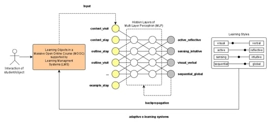
The algorithm chosen for multi-target prediction was artificial neural network (ANN) for five reasons: (a) there is evidence that this algorithm is better suited to solve learning style classification problems [5]; (b) since many authors use this algorithm, we can compare our results with other published ones [3]; (c) ANN works well with rather small datasets, which is important for this line of research considering that typical datasets are rather small [17]; (d) the problem can be translated to the network structure of an ANN; and (e) ANN allows multiple outputs analyzed at the same time. Moreover, the ANN architecture we used is feedforward multilayer perceptron, which means a neural network with one or more hidden layers [17,20].

The hidden layers act as feature detectors; as such, they play an important role in the operation of a multilayer perceptron. As the learning process advances throughout the multilayer perceptron, step by step the hidden neurons start to discover the features that describe the training data. They do so by performing nonlinear processing on the input data and transforming them into a new space, called the feature space. In this new space, the classes of interest in a pattern-classification task, for instance, may be more easily separated from each other than they could in the original input data space. Indeed, it is the creation of this feature space through supervised learning which distinguishes the multilayer perceptron from perceptron. Literature suggests that the number of hidden layers should be between log T (where T is the size of the training set) and 2× the number of inputs [17].

A popular approach for training multilayer perceptron is the back-propagation algorithm, which incorporates the least mean squares (LMS) algorithm as a special case. The training proceeds in two steps. In the first one, referred to as the forward phase, the synaptic weights of the network are updated and the input signal is propagated through the network, layer by layer, until the output. As a consequence, in this phase, adjustments are limited to the activation potentials and outputs of the neurons in the network. (b) In the second one, called the backward phase, an error signal is produced by evaluating the output of the network with an expected response. The resulting error signal is propagated through the network, again layer by layer, but this time the propagation is performed in the backward direction. In this second step, successive updates are made to the synaptic weights of the network. Calculation of the updates for the output layer is straightforward, but it is much more difficult for the hidden layers [17].

The back-propagation algorithm affords an approximation to the trajectory in weight space computed by the method of the stochastic gradient descent [17]. The smaller the value of the learning rate parameter α, the smaller the changes to the synaptic weights in the network. Consequently, it will be from the first iteration to the next in a smoother fashion during the trajectory in weight space. This improvement, however, is attained at the cost of a slower rate of learning. The learning rates used were between 0.01 and 0.1, in steps of 0.01, leading to the following values: (0.01, 0.02, 0.03, 0.04, 0.05, 0.06, 0.07, 0.08, 0.09, 0.1) [17].

A training set is one of labeled data (for example, if a student is active or reflective) providing known information, which is used in supervised learning to build a classification or regression model. The training dataset is used to train the model (weights and biases in the case of artificial neural network) and then the model can see and learn from this data.

The model test is a critical but frequently underestimated part of model building and assessment. After preprocessing the data, they are needed to build a model with the potential to accurately predict further observations. If the built model completely fits the training data, it is probably not reliable after deployment in the real world. This problem is called overfit and needs to be avoided. A common manner on how to address the lack of an independent dataset for model evaluation is to reserve part of the learning data for this purpose. The basis for analyzing classifier performance is a confusion matrix (CF). This matrix describes how well a classifier can predict classes.

A typical cross validation technique is the k-fold cross validation. This method can be viewed as a recurring holdout method (holdout method divides the original dataset in two subsets, training and testing datasets). The whole data is divided into k equal subsets and each time a subset is assigned as a test set, the others are used for training the model. Thus, each observation gets a chance to be in the test and training sets; therefore, this method reduces the dependence of performance on test–training split and decreases the variance of performance metrics. Further, the extreme case of k-fold cross validation will occur when k is equal to the number of data points. It would mean that the predictive model is trained over all the data points except by one, which takes the role of a test set. This method of leaving one data point as a test set is known as leave-one-out cross validation (LOOCV) [17]. This technique is show in Figure 4.

As shown in Figure 4, each iteration leaves one observation to test and the others to train. Therefore, the number of iterations is the number of observations in the dataset. The use of the leave-one-out procedure allows the model to be tested with all observations and prevents us from wasting these observations. This method was used to split the original dataset.

A classifier is evaluated based on performance metrics computed after the training process. In a binary classification problem, a matrix presents the number of instances predicted by each of the four possible outcomes: number of true positives (#TP), number of true negatives (#TN), number of false positives (#FP), and number of false negatives (#FN). Most classifier performance metrics are derived from the four values [21]. We used the following metrics in order to improve the accuracy of our model (Equations (3)–(14)) [22].

$$\mathrm{Sensitivity} =\frac{\mathrm{TP}}{\mathrm{TP}+\mathrm{FP}}$$

(3)

$$\mathrm{Specificity} =\frac{\mathrm{TN}}{\mathrm{FN}+\mathrm{TN}}$$

(4)

$$\mathrm{Prevalence} =\frac{\mathrm{TP}+\mathrm{FP}}{\mathrm{TP}+\mathrm{FN}+\mathrm{FP}+\mathrm{TN}}$$

(5)

$$\mathrm{PPV} =\frac{\mathrm{sensitivity} \ast \mathrm{prevalence}}{\left(\mathrm{sensitivity}\ast \mathrm{prevalence}\right)+\left(\left(1-\mathrm{specificity}\right)\ast \left(1-\mathrm{prevalence}\right)\right)}$$

(6)

$$\mathrm{NPV} =\frac{\mathrm{specificity}\ast \left(1-\mathrm{prevalence}\right)}{\left(\left(1-\mathrm{sensitivity}\right)\ast \mathrm{prevalence}\right)+\left(\left(1-\mathrm{specificity}\right)\ast \left(1-\mathrm{prevalence}\right)\right)}$$

(7)

$$\mathrm{Detection} \mathrm{Rate} =\frac{\mathrm{TP}}{\mathrm{TP}+\mathrm{FN}+\mathrm{FP}+\mathrm{TN}}$$

(8)

$$\mathrm{Detection} \mathrm{Prevalence} =\frac{\mathrm{TP}+\mathrm{FN}}{\mathrm{TP}+\mathrm{FN}+\mathrm{FP}+\mathrm{TN}}$$

(9)

$$\mathrm{Balanced} \mathrm{Accuracy} =\frac{\mathrm{sensitivity}+\mathrm{specificity}}{2}$$

(10)

$$\mathrm{Precision} =\frac{\mathrm{TP}}{\mathrm{TP}+\mathrm{FN}}$$

(11)

$$\mathrm{Recall} =\frac{\mathrm{TP}}{\mathrm{TP}+\mathrm{FP}}$$

(12)

$$\mathrm{F}1 =\frac{\left(1+{\mathsf{\alpha }}^2\right)\ast \mathrm{precicion}\ast \mathrm{recall}}{\left({\mathsf{\alpha }}^2\ast \mathrm{precision}\right)+\mathrm{recall}}$$

(13)

$$\mathrm{Accuracy} =\frac{\mathrm{TP}+\mathrm{TN}}{\mathrm{TP}+\mathrm{FP}+\mathrm{TN}+\mathrm{FN}}$$

(14)

For binary problems, the sensitivity, specificity, positive predictive value, and negative predictive value were calculated using the positive argument. The overall method is shown in Figure 5.

As shown in Figure 5, the behavior of the 100 students is presented to the Multi Layer Perceptron (MLP) in order to train the neural network. The weight of each synapse (neuron connection) is obtained and the result is compared to the expected outcome (Equations (3)–(14)). When the accuracy (shown in

Table 3. Metrics of each dimension.

Processing (Active_Reflective)	Perception (Sensing_Intuitive)
Accuracy: 0.85	Accuracy: 0.76
95% CI: (0.2306, 0.6847)	95% CI: (0.3605, 0.8088)
No Information Rate: 0.6	No Information Rate: 0.55
p-Value (Acc > NIR) 1: 0.9435	p-Value (Acc > NIR): 0.4143
Kappa: −0.0784	Kappa: 0.1919
Mcnemar’s Test p-Value: 0.5465	Mcnemar’s Test p-Value: 1.0000
Sensitivity: 0.5000	Sensitivity: 0.5556
Specificity: 0.4167	Specificity: 0.6364
Pos Pred Value: 0.3636	Pos Pred Value: 0.5556
Neg Pred Value: 0.5556	Neg Pred Value: 0.6364
Prevalence: 0.4000	Prevalence: 0.4500
Detection Rate: 0.2000	Detection Rate: 0.2500
Detection Prevalence: 0.5500	Detection Prevalence: 0.4500
Balanced Accuracy: 0.4583	Balanced Accuracy: 0.5960
‘Positive’ Class: 1	‘Positive’ Class: 1
Input (Visual_Verbal)	Understanding (Sequential_Global)
Accuracy: 0.75	Accuracy: 0.80
95% CI: (0.4078, 0.8461)	95% CI: (0.1912, 0.6395)
No Information Rate: 0.65	No Information Rate: 0.65
p-Value [(Acc > NIR): 0.601	p-Value (Acc > NIR): 0.9940
Kappa: 0.2045	Kappa: −0.2371
Mcnemar’s Test p-Value: 1.000	Mcnemar’s Test p-Value: 0.7728
Sensitivity: 0.7692	Sensitivity: 0.4615
Specificity: 0.4286	Specificity: 0.2857
Pos Pred Value: 0.7143	Pos Pred Value: 0.5455
Neg Pred Value: 0.5000	Neg Pred Value: 0.2222
Prevalence: 0.6500	Prevalence: 0.6500
Detection Rate: 0.5000	Detection Rate: 0.3000
Detection Prevalence: 0.7000	Detection Prevalence: 0.5500
Balanced Accuracy: 0.5989	Balanced Accuracy: 0.3736
‘Positive’ Class: 1	‘Positive’ Class: 1

¹ NIR and ACC represent, respectively, No Information Rate (NIR) and Accuracy (ACC).

) is optimal (i.e., without improvement during the training step), the neural network training stops. The pseudocode that explains this method is presented below.

Pseudocode 1: The overall idea of method to learning style classification

$accuracy=0$

$variation=max$

$while\left(variation>0.01\right)\{$

$present the subset of train and test to MLP$

$weights=weights-delta\_weights\ast learning\_rate$

$compare the predicted outcome to expected$

$variation=the diference of the predicted and expected$

$update accurary$

$\}$

As shown in Pseudocode 1 all the subsets (train and test) are presented to the MLP to train and test. Accuracy is one of the metrics of Table 3 that is used to build the model, avoiding overfitting and underfitting [17].

4. Discussion

In this section, the results from the experiments are presented and discussed. We initially investigated the aspects of three types of variables: (a) count descriptors, (b) time descriptors, and (c) target descriptors where, this last one is of type count. There were no outliers found in the dataset. The median of the type count descriptors was around four accesses by the element (content_visit, outline_visit, etc.), as shown in Figure 4. The time descriptors define the time spent in each element (content_stay, outline_stay, etc.). The zero (0) value represents that the element had no access. The median time spent in type time was around 60 s and there was restriction that limited access at 120 s because of a time session limit. Finally, the target variables’ median was around 0, which express the balanced learning styles dataset in each dimension (input, processing, perceive, and store), which means that the students are about evenly distributed between active and reflexive classes. These values are shown in Figure 6.

We also explored the frequency from each preference dimension before target transformation into binary variables (Equation (2)). As a result, we obtained the students’ learning styles for each dimension. The dimensions active_reflective, sensing_intuitive, and sequential_global presented an approximately uniform distribution; however, the visual_verbal dimension presented a concentration close to −5, which represents a preference by the students to acquire visual information. Figure 7 shows this analysis.

We also investigated the possibility of using the dataset to identify students’ preferences. If, for example, a determined set of attributes represents one of the four learning dimensions, these attributes may help in the dimensionality reduction and improve classifier precision [7,16]. The groups were investigated using the k-means algorithm to identify natural clusters in dataset. The k-means algorithm was used with k = {2, 3, 4, 5}. As a result, we obtained clusters with two and three groups with low overlap. By using a number of groups up to three, the resulting clusters overlapped. These results are shown in Figure 8.

Additionally, another analytics technique, known as principal component analysis (PCA), was applied to investigate other relevant attributes or correlations and whether targets, of each dimension, might be explained by some descriptor (count and time). This is an important issue for dimensionality reduction in order to improve accuracy and reduce the cost of the model build [20]. These results are shown in Figure 9.

The dataset is balanced for the dimensions perceive, processing, and store, and presents some variation in the dimension input. In addition, there is not a predominant descriptor, making it possible to use all descriptors for the model construction.

We may identify the onset of overfitting through the use of leave-one-out (special case of k-fold cross validation), for which the training data are split into an estimation subset and a validation subset. The estimation subset of examples is used to train the network in the usual way, except for a minor modification; the training session is stopped periodically (i.e., every so many epochs), and the network is tested on the validation subset after each period of training.

In our procedure, we varied the numbers of hidden layers for each model to determine a suitable number and provide the optimal result. The best model built presents two hidden layers, 26 neurons of input, and four neurons of output. The resulting model is shown in Figure 10.

This model evaluates all descriptors, simultaneously providing the students’ classification in each learning dimension. This is a multi-target prediction algorithm [19]. Equations (4)–(14) were used to evaluate the model. We used the confusion matrix (CF) [17] to classify the predictions. The results of each dimension are shown in Table 3.

The best model built achieved 85%, 76%, 75%, and 80% accuracy in each target attribute, active_reflective, sensing_intuitive, visual_verbal, and sequential_global, respectively. These results are better than the results presented by Bernard et al. [5] (80%, 74%, 72%, and 82% in the same order) except for sequential_global, and simultaneously deal with all descriptors and targets instead of one at a time; we generated one model while Bernard et al. [5] generated four models to solve the problem. Moreover, we provided many performance metrics for each dimension to support further research to compare and improve their results (Table 3). In addition, we investigated the CF using area under the curve (AUC) and receiver operating characteristics (ROC). For each target the results were superior to Bernard et al. [5]. Figure 11 shows these results.

All metrics indicated that the model might be a method to automatically classify a student in a MOOC environment. The relation between descriptors improves the accuracy (as show in specificity and sensitivity from Table 3). Moreover, multi-target prediction (MTP) is a class of algorithms used with the simultaneous prediction of multiple target variables of diverse types, and the model using the Felder–Silverman procedure is by far, the most popular theory applied in adaptive e-learning system [5]. Meanwhile, from another point of view, the accuracy (and other performance metrics) of the outcomes using the proposed approach could be further improved by the use of a big dataset. Another limitation of the current research is that the results of the experiments were only tested on a platform with a specific subject (computer science and project management). The consistency of performance needs to be tested when it runs with different learning management systems and/or other online courses (for example, administration, economics, and so forth). Our future work will involve further exploration of the performance metrics and practical implications in different environments.

5. Conclusions and Further Development

This paper presents an automatic approach to identify learning styles of student behavior in a MOOC using a Computer Intelligent Algorithm (CIA) called deep artificial neural network (ANN). Assessment with the data of 100 students was performed, demonstrating the overall accuracy of the approach for each of the four Felder–Silverman learning styles model (FSLSM) learning style dimensions. It can be observed from the results obtained that this approach may be used to identify students’ learning style based on their behavior in MOOC. This approach reduces the noise of questionnaires [3,4,5], allows classification when necessary to check if the style has changed over time [1], and allows data to be stored for future use.

Thus, by identifying students’ learning styles, adaptive learning systems can use this information to provide more accurate personalization, leading to improved satisfaction and reduced learning time [3]. In addition, students can directly benefit from the more accurate identification of the learning styles, being able to leverage their strengths in relation to learning styles and understanding their weaknesses. In addition, teachers can use this learning style information to provide students with more accurate advice, which, as pointed out before, becomes more useful for students as learning style identification becomes more accurate as well. Moreover, students with similar learning styles may work together in the same classroom to improve their learning experience and help the teachers with their methods. Additionally, other stakeholders in the education ecosystem, such as parents, teachers, and administrators, can make use of such an approach to improve education in general [2,21].

Suggestions to further works may include the practical application of this approach through MOOC plug-ins. Different algorithms can be tested by comparing their results with works of the artificial neural network, since this work presents reference values based on the confusion matrix that can be replicated to other algorithms. Social issues can also be investigated to identify whether they influence learning styles. Concept drift (CD) should be investigated to identify if the target variables modify over time and compare the results to learning process questionnaires (LPQs). Finally, we may investigate how learning styles work in the propagation of information in networks based on complex networks [17]. This is an important topic, with great impact in real-world applications because it is a base to recommendation systems, and may be used to improve students’ learning processes.

References

1. Willingham, D.T. Why Don’t Students Like School? A Cognitive Scientist Answers Questions about How the Mind Works and What It Means for the Classroom; Jossey-Bass: San Francisco, CA, USA, 2010. [Google Scholar]
2. Felder, R.M.; Silverman, L.K. Learning and teaching styles in engineering education. Eng. Educ. 1988, 78, 674–681. [Google Scholar]
3. Afini Normadhi, N.B.; Shuib, L.; Md Nasir, H.N.; Bimba, A.; Idris, N.; Balakrishnan, V. Identification of personal traits in adaptive learning environment: Systematic literature review. Comput. Educ. 2019, 130, 168–190. [Google Scholar] [CrossRef]
4. Pashler, H.; Mcdaniel, M.; Rohrer, D.; Bjork, R. Concepts and Evidence. Psychol. Sci. Public Interest 2009, 9, 105–119. [Google Scholar] [CrossRef] [PubMed] [Green Version]
5. Bernard, J.; Chang, T.W.; Popescu, E.; Graf, S. Learning style Identifier: Improving the precision of learning style identification through computational intelligence algorithms. Expert Syst. Appl. 2017, 75, 94–108. [Google Scholar] [CrossRef]
6. Kolb, Y.A.; Kolb, A.D. Learning Styles and Learning Spaces: Enhancing Experiential Learning in Higher Education. Acad. Manag. Learn. Educ. 2016, 4, 193–212. [Google Scholar] [CrossRef] [Green Version]
7. Truong, H.M. Integrating learning styles and adaptive e-learning system: Current developments, problems and opportunities. Comput. Hum. Behav. 2016, 55, 1185–1193. [Google Scholar] [CrossRef]
8. Omar, N.; Mohamad, M.M.; Paimin, A.N. Dimension of Learning Styles and Students’ Academic Achievement. Procedia Soc. Behav. Sci. 2015, 204, 172–182. [Google Scholar] [CrossRef] [Green Version]
9. Rasheed, F.; Wahid, A. Learning Style Recognition: A Neural Network Approach. In First International Conference on Artificial Intelligence and Cognitive Computing, Advances in Intelligent Systems and Computing; Springer: Singapore, 2019; Volume 815, pp. 301–312. [Google Scholar] [CrossRef]
10. Graf, S.; Liu, T.; Graf, S.; Liu, T. Supporting Teachers in Identifying Students’ Learning Styles in Learning Management Systems: An Automatic Student Modeling Approach. Int. Forum Educ. Technol. Soc. 2016, 12, 2–14. [Google Scholar]
11. Saryar, S.; Kolekar, S.V.; Pai, R.M.; Pai, M.M.M. Mobile Learning Recommender System Based on Learning Styles. In Soft Computing and Signal Processing, Advances in Intelligent Systems and Computing; Springer: Singapore, 2019; Volume 898, pp. 299–312. [Google Scholar] [CrossRef]
12. Ahmad, N.; Tasir, Z.; Kasim, J.; Sahat, H. Automatic Detection of Learning Styles in Learning Management Systems by Using Literature-based Method. Procedia Soc. Behav. Sci. 2013, 103, 181–189. [Google Scholar] [CrossRef] [Green Version]
13. El-Bishouty, M.M.; Aldraiweesh, A.; Alturki, U.; Tortorella, R.; Yang, J.; Chang, T.W.; Graf, S. Use of Felder and Silverman learning style model for online course design. Educ. Technol. Res. Dev. 2019, 67, 161–177. [Google Scholar] [CrossRef]
14. Sheeba, T.; Krishnan, R. Automatic Detection of Students Learning Style in Learning Management System. In Smart Technologies and Innovation for a Sustainable Future, Advances in Science; Springer International Publishing: New York, NY, USA, 2019; pp. 45–53. [Google Scholar] [CrossRef]
15. Li, L.X.; Soraya, S.; Rahman, A. Students’ learning style detection using tree augmented naive Bayes. R. Soc. Open Sci. 2018, 5, 17210. [Google Scholar] [CrossRef] [PubMed] [Green Version]
16. Franzoni, A.L.; Assar, S. Student learning styles adaptation method based on teaching strategies and electronic media. Educ. Technol. Soc. 2009, 12, 15–29. [Google Scholar]
17. Soudry, D.; di Castro, D.; Gal, A.; Kolodny, A.; Kvatinsky, S. Memristor-Based Multilayer Neural Networks with Online Gradient Descent Training. IEEE Trans. Neural Netw. Learn. Syst. 2015, 26, 2408–2421. [Google Scholar] [CrossRef] [PubMed]
18. Rout, N.; Mishra, D.; Mallick, M.K. Handling imbalanced data: A survey. Adv. Intell. Syst. Comput. 2018, 628, 431–443. [Google Scholar] [CrossRef]
19. Index of Learning Styles Questionnaire. Available online: https://www.webtools.ncsu.edu/learningstyles/ (accessed on 29 February 2020).
20. Liu, Y.-Y.; Slotine, J.-J.; Barabási, A.-L. Controllability of complex networks. Nature 2011, 473, 167–173. [Google Scholar] [CrossRef] [PubMed]
21. Gomede, E.; Gaffo, F.H.; Briganó, G.U.; de Barros, R.M.; Mendes, L.S. Application of Computational Intelligence to Improve Education in Smart Cities. Sensors 2018, 18, 267. [Google Scholar] [CrossRef] [PubMed] [Green Version]
22. Kuhn, M. Building predictive models in R using the caret package. J. Stat. Softw. 2008, 28, 1–26. [Google Scholar] [CrossRef] [Green Version]
Figure 1. The process to build a model for automatic detection of learning style [5]. In this paper, we aim to investigate the steps a, b, and c. MOOC = massive open online course.
Applsci 10 01756 g001
Figure 2. The process to build the dataset (independent and dependent variables). The questionnaire was used to label the dataset for each student’s observation.
Applsci 10 01756 g002
Figure 3. The dataset’s target distribution of each dimension. The % of each student’s preferences are represented, such a, sequential 42%, global 58%, visual 38%, verbal 62%, sensing 45%, intuitive 55%, active 49%, and reflective 51%.
Applsci 10 01756 g003
Figure 4. Leave-one-out cross validation technique (LOOCV). It is a special case of cross validation where the number of folds equals the number of instances in the dataset [17].
Applsci 10 01756 g004
Figure 5. The overall method for learning styles classification based on count and time descriptors and targets. The behavior of the student is presented to the Multi Layer Perceptron (MLP) to train and get the weights which explain the labeled dataset.
Applsci 10 01756 g005
Figure 6. Box plot analysis of dataset (count and time descriptors and targets). There is a limitation to the time descriptor by 120 s and count by 10 times.
Applsci 10 01756 g006
Figure 7. Learning style frequency distribution of each dimension.
Applsci 10 01756 g007
Figure 8. Natural clusters in dataset using k-means (with k = {2, 3, 4, 5}). No natural cluster was identified and, therefore, the classes are not linearly separated.
Applsci 10 01756 g008
Figure 9. Principal component analysis (PCA) of each dimension, processing, perception, input, and understanding, respectively.
Applsci 10 01756 g009
Figure 10. The built model with 2 hidden layers, 26 neurons of input, and 4 neurons of output.
Applsci 10 01756 g010
Figure 11. The receiver operating characteristics (ROC) analysis of each confusion matrix dimension that illustrates the diagnostic ability of the binary classifier system as its discrimination threshold is varied. (a) Represents the individual confusion matrix and (b) represents the individual ROC curve.
Applsci 10 01756 g011