Semantic 3D Reconstruction with Learning MVS and 2D Segmentation of Aerial Images

Abstract

Semantic modeling is a challenging task that has received widespread attention in recent years. With the help of mini Unmanned Aerial Vehicles (UAVs), multi-view high-resolution aerial images of large-scale scenes can be conveniently collected. In this paper, we propose a semantic Multi-View Stereo (MVS) method to reconstruct 3D semantic models from 2D images. Firstly, 2D semantic probability distribution is obtained by Convolutional Neural Network (CNN). Secondly, the calibrated cameras poses are determined by Structure from Motion (SfM), while the depth maps are estimated by learning MVS. Combining 2D segmentation and 3D geometry information, dense point clouds with semantic labels are generated by a probability-based semantic fusion method. In the final stage, the coarse 3D semantic point cloud is optimized by both local and global refinements. By making full use of the multi-view consistency, the proposed method efficiently produces a fine-level 3D semantic point cloud. The experimental result evaluated by re-projection maps achieves 88.4% Pixel Accuracy on the Urban Drone Dataset (UDD). In conclusion, our graph-based semantic fusion procedure and refinement based on local and global information can suppress and reduce the re-projection error.

1. Introduction

Semantic 3D reconstruction makes Virtual Reality (VR) and Augmented Reality (AR) much more promising and flexible. In computer vision, 3D reconstruction and scene understanding receive more and more attention these days. 3D models with correct geometrical structures and semantic segmentation are crucial in urban planning, automatic piloting, robot vision, and many other fields. For urban scenes, semantic labels are used to visualize targets such as buildings, terrain, and roads. A 3D point cloud with semantic labels makes the 3D map more simple to understand, thereby propelling the subsequent research and analysis. 3D semantic information also shows potential in automatic piloting. For a self-driving vehicle, one of the most important things is to distinguish whether the road is passable or not. Another essential thing for an autonomous automobile is to localize other vehicles in real-time so that it can adapt to their speed, or exceed it if necessary. In the field of robotics, scene understanding is a standard task for recognizing surrounding objects. The semantics of the surrounding environment play a vital role in applications such as loop closure and route planning.

Although 3D semantic modeling has been widely studied in recent years, the approaches of extracting semantic information through the post-processing of point cloud reconstruction generally lead to inconsistent or incorrect results. Performing semantic segmentation on point cloud data is more difficult than it is on 2D images. One major problem is the lack of 3D training data, since labeling a dataset in 3D is much more laborious than in 2D. Another challenge is the unavoidable noise in 3D point clouds, which makes it difficult to accurately distinguish which category a point belongs to. Thus, it is necessary to develop new semantic 3D reconstruction approaches by simultaneously estimating 3D geometry and semantic information over multiple views. In the past few years, many studies on image semantic segmentation have achieved promising results by deep learning techniques [1,2,3,4]. Deep learning methods based on well-trained neural networks can help us do pixel-wise semantic segmentation on various images. Meanwhile, deep-learning-based methods are not only able to extract semantic information, but are also practical for solving Multi-View Stereo (MVS) problems. Recently, learning-based MVS algorithms [5,6] have been proposed to generate high precision 3D point clouds for large-scale scenes. These results inspired us much and gave rise to the research of semantic 3D reconstruction. In this paper, we mainly focus on developing accurate, clear, and complete 3D semantic models of urban scenes.

Once satisfactory depth and semantic maps are acquired, 3D semantic models can be easily generated. 3D laser scanners can detect depth directly but only perform well in short-distance indoor scenes. Compared with 3D laser scanners, the purely RGB-based method to reconstruct 3D models from 2D images is cheaper, faster, and more generalized. Recently, Unmanned Aerial Vehicles (UAV) have become applicable to collecting multi-view, high-resolution aerial images of large-scale outdoor scenes. The calibrated camera poses can be obtained from the images by the traditional Structure from Motion (SfM) technique. After that, 3D point clouds are determined by fusing 2D images according to multi-view geometry.

However, due to the occlusions, the complexity of environments, and the noise of sensors, both 2D segmentation and depth estimation results contain errors. As a result, many inconsistencies may occur when projecting the multi-view 2D semantic labels to the corresponding 3D points. There is still plenty of work to do to obtain accurately-segmented 3D semantic models. With the booming of deep learning methods, 2D segmentation tasks are reaching high performance levels, which makes it possible to acquire a large-scale 3D semantic model easily. Nevertheless, errors within depth maps and semantic maps may lead to inconsistency. This can be alleviated by considering 3D geometry and 2D confidence maps together in an optimization module. Moreover, 3D models with coarse segmentation still need further refinement to filter error points. In a nutshell, the main contributions of our work are three folds:

• We present an end-to-end, learning-based, semantic 3D reconstruction framework, which reaches high Pixel Accuracy on the Urban Drone Dataset (UDD) [7].
• We propose a probability-based semantic MVS method, which combines the 3D geometry consistency and 2D segmentation information to generate better point-wise semantic labels.
• We design a joint local and global refinement method, which is proven effective by computing re-projection errors.

2. Related Work

Right before the renaissance of deep learning, it was a hard task to get a good pixel-wise segmentation map on images. Bao, S.Y. et al. [8] take object-level semantic information to constrain camera extrinsic. Some other methods perform the segmentation directly on the point cloud or meshes, according to their geometric characteristics. Martinovic, A. et al. [9] and Wolf, D. et al. [10] take the random forest classifier to do point segmentation, while Häne, C. et al. [11,12] and Savinov, N. et al. [13] treat it as an energy minimization problem in a Conditional Random Field (CRF). Ray potential (likelihood) is frequently adopted in semantic point cloud generation.

The flourishing CNN-based semantic segmentation methods are quickly outperforming traditional methods in image semantic segmentation tasks; take, for example, the Fully Convolutional Network (FCN) [1] and Deeplab [3]. High-level computer tasks such as scene understanding and semantic 3D reconstruction are now steady and rudimentary processes. The goal of 3D semantic modeling is to assign a semantic label to each 3D point rather than each 2D pixel. Several learning-based approaches follow the end-to-end manner, analyzing the point cloud and giving segmentation results directly in 3D. Voxel-based methods such as ShapeNets [14] and VoxNet [15] were proposed naturally. Some methods learn a spatial encoding of each point and then aggregate all individual point features to a global point cloud signature [16,17]. However, current deep learning-based segmentation pipelines cannot handle noisy, large-scale 3D point clouds. Thus, a feasible method is required to firstly perform pixel-wise semantic segmentation on 2D images and then back-project these labels into 3D space using the calibrated cameras to be fused. The methods above handle the point cloud directly, which means they carry a costly computational burden. In other words, they cannot manage large-scale 3D scenes without first partitioning the scene. More than that, because the morphological gap between point clouds in different scenarios is too large. These algorithms may be poorly generalized.

There are several methods doing semantic segmentation on 2D image and making use of multi-view geometric relationships to project semantic labels into 3D space. For RGBD-based approaches, once good semantic maps of each image are acquired, the semantic point clouds can easily be fused. Vineet, V. et al. [18] took advantage of a random forest to classify 2D features to get semantic information, while Zhao, C. et al. [19] used FCN with CRF-RNN to perform segmentation on images. McCormac, J. et al. [20] and Li, X. et al. [21] proposed incremental semantic label fusion algorithms to fuse 3D semantic maps. For RGB-based approaches, also addressed as Structure from Motion (SfM) and MVS, each point in the generated 3D structure corresponds to pixels on several images. Following the prediction of 2D labels, the final step is to assign each 3D pixel a semantic label [20,22]. The refinement process is as essential as the generation process of the semantic point cloud itself. Chen, Y. et al. [7] and Stathopoulou, E.K. et al. [23] filter the mismatching by semantic labels of feature points. With the motivation of denoising, Zhang, R. et al. [24] proposed a Hough-transform-based algorithm called FC-GHT to detect plane on point cloud for further semantic label optimization. Stathopoulou, E.K. et al. [23] used semantic information as a mask to wipe out the meshes belonging to the semantic class sky. These methods have two primary drawbacks. Firstly, they only use the final semantic maps, which means the probabilities of other categories are discarded. Secondly, they contain no global constraints integrated into their algorithms. In response, we propose some ideas for improvement.

3. Method

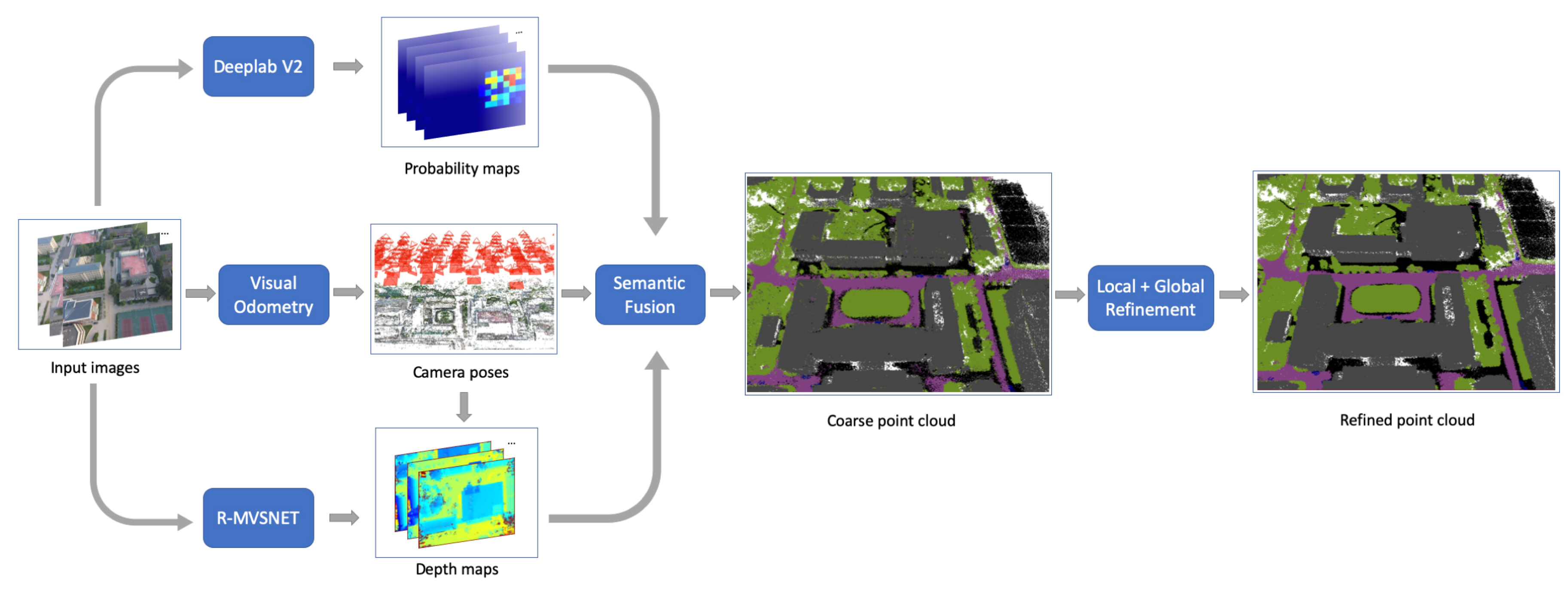
3.1. Overall Framework

The overall framework of our method is depicted in Figure 1. In the Deeplab v2 [3]-based 2D segmentation branch, we discard the last Argmax layer of the network. We save pixel-wise semantic probability maps for every image instead. With the help of COLMAP-SfM [25], we simultaneously estimate the camera parameters and depth ranges for the source images. In order to acquire 3D geometry for large scale scenes, we utilize learning-based MVS method R-MVSNet [6] to estimate depth maps for multiple images. After 2D segmentation and depth estimation, we obtain a dense semantic point cloud by the semantic fusion method according to multi-view consistency. Finally, we propose a graph-based point cloud refinement algorithm integrating both local and global information as the last step of our pipeline.

3.2. 2D Segmentation

In this research, Deeplab v2 [3] with Residue Block is adopted as our segmentation network. The pretrained weights of ResNet-101 [26] on Imagenet [27] are used as our initial weights. We adopt the residual block to replace the ordinary 2D convolution layer to improve the training performance. We also modify the softmax layer that classifies the images to fit the label space of the UDD [7] dataset. With the network all set up, the training set of UDD [7] is employed for transfer learning.

The label space of UDD [7] is denoted as $\mathcal{L}=\{l_0,l_1,l_2,l_3,l_4\}$, which contains Vegetation, Building, Road, Vehicle, and Background. After the transfer learning process, we predict the semantic maps for every image in the reconstruction dataset. Furthermore, we save the weight matrix before the last Argmax layer. This matrix $\mathbf{P}(\mathcal{L})$ represents the probability distributions of every pixel in the semantic label space.

3.3. Learning-Based MVS

In order to acquire 3D geometry for large scale scenes, we explore the learning-based MVS method to estimate depth maps for multiple images. R-MVSNet [6], a deep learning architecture with capability to handle multi-scale problem, has advantages in processing high-resolution images and large-scale scenes. Moreover, R-MVSNet utilizes the Gated Recurrent Unit (GRU) to sequentially regularize the 2D cost maps, which reduces the memory consumption and makes the network flexible. Thus, we follow the framework of R-MVSNet to generate corresponding depths of the source images and train it on the DTU [28] dataset. Camera parameters and image pairs are determined by the implementation of COLMAP-SfM [25], while depth samples are chosen within $[d_{min},d_{max}]$ using the inverse depth setting. The network returns a probability volume $\mathit{P}$ where $P(x,y,d)$ is the probability estimation for the pixel $(x,y)$ at depth d; then, the expectation depth value $d(x,y)$ is calculated by the probability weighted sum over all hypotheses:

$$d(x,y)=\sum _{d=d_{min}}^{d_{max}}P(x,y,d)·d.$$

(1)

However, as with most depth estimation methods, the coarse pixel-wise depth data $d(x,y)$ generated by R-MVSNet may contain errors. Therefore, before point cloud fusion by the depth maps, it is necessary to perform a denoising process on the depth data. In this paper, we apply the bilateral filtering method to improve the quality of depth maps with edge preservation; the refined depth data $d^{\prime }(x,y)$ are obtained by:

$$d^{\prime }(x,y)=\frac{{\sum }_{i,j}\omega (x,y,i,j)·d(x,y)}{{\sum }_{i,j}\omega (x,y,i,j)}$$

(2)

where $\omega (x,y,i,j)=exp(-\frac{{(x-i)}^2+{(y-j)}^2}{2{\sigma }_f^2}-\frac{{\left|\left|d(x,y)-d(i,j)\right|\right|}^2}{2{\sigma }_g^2})$ is the weighted coefficient; ${\sigma }_f$ and ${\sigma }_g$ are the variance of domain kernel $f(x,y,i,j)=exp(-\frac{{(x-i)}^2+{(y-j)}^2}{{\sigma }_f^2})$ and range kernel $g(x,y,i,j)=exp(-\frac{{\left|\left|d(x,y)-d(i,j)\right|\right|}^2}{{\sigma }_g^2})$ respectively. As shown in Figure 2, the depth map becomes more smooth with edge preservation after bilateral filtering.

3.4. Semantic Fusion

With the learning 2D segmentation and depth estimation, pixel-wise 2D semantic labels and depth maps are obtained for each view. However, because of the occlusions, complexities of environments, and the noise of sensors, both image segmentation results and depth maps might have a large number of inconsistencies between different views. Thus, we further cross filter the depth maps by their neighbor views, and then produce the 3D semantic point clouds by combining 2D segmentation and depth maps with multi-view consistency.

Similar to other depth-map-based MVS methods [6,29], we utilize geometric consistency to cross filter the multi-view depth data. Given the pixel $(x,y)$ from image $I_i$ with depth $d(x,y)$, we project $(x,y)$ to the neighbor image $I_j$ through $d(x,y)$ and camera parameters. In turn, we re-project the projected pixel back from the neighbor image $I_j$ to the original image $I_i$; the re-projected depth on $I_i$ is $d_{reproj}$. We consider the pixel consistent in the neighbor view $I_j$ when $d_{reproj}$ satisfies:

$$\frac{\left|d(x,y)-d_{reproj}\right|}{d(x,y)}<\tau .$$

(3)

According to the geometric consistency, we filter the depths which are not consistent in more than k views. In this paper, we take $\tau =0.01$ and $k=3$.

After cross filtering, the depths are projected to 3D space to produce 3D point clouds. Since our purpose is to assign point-wise semantic labels for the 3D model, we propose a probabilistic fusion method to aggregate multi-view 2D semantic information. With the fine-tuned CNN, a pixel-wise label probability distribution $\mathbf{P}(\mathcal{L})$ has been calculated for each source image. Given a 3D point X which is visible in N views, the corresponding probability on view i for label $l_j$ is $p_i(l_j)$; we accumulate the multi-view probability distribution of each view as follows:

$$P(l_j)=\frac{1}{N}\sum _{i=1}^N{p}_i(l_j),l_j\in \mathcal{L},$$

(4)

where $P(l_j)$ denotes the probability of point X labeling by $l_j$. In this way, we transfer the probability distribution of multi-view images into 3D space. Generally, the predicted 3D semantic label can be determined by the Argmax operation as:

$$l(X)=\underset{l_j}{Argmax}(P(l_j)),l_j\in \mathcal{L},$$

(5)

where $l(X)$ is the 3D semantic label of X. As depicted in Figure 3, the probabilistic fusion method effectively reduces errors since it integrates information from multiple images.

3.5. Point Cloud Refinement

Through the semantic fusion method, the 3D point cloud is classified into point-wise semantic labels. However, there are still few scattered points with error labels due to incorrect semantics or depths of source images. To remove these unexpected semantic errors, we explore both local and global refinement strategies for point cloud refinement. The KD-Tree data structure is employed to accelerate the query speed of the point cloud from O(n) to O(log(n)).

Generally, adjacent point clouds often have some correlation and are more likely to be segmented into the same class. Hence, we utilize the local refinement method for each point by combining the hypothesizes with the neighbor points. Given a 3D point X from the dense semantic model, through the KD-Tree structure established by the whole point cloud, the k-nearest neighbor of X could be determined in a short time. $P_i(l_j),i=1,\cdots ,k$ represents the probability for neighbor point i labeling by $l_j$; the new semantic label $l^{\prime }(X)$ is updated by:

$$l^{\prime }(X)=\underset{l_j}{Argmax}(\frac{1}{k}\sum _{i=1}^k{P}_i(l_j)),l_j\in \mathcal{L}.$$

(6)

However, the local refinement method only takes the local adjacency into consideration with the global information ignored. For overall optimization, we further apply a graph-based global refinement method by minimizing an energy function. For every 3D point in the point cloud $\mathbf{V}$, a graph $\mathbf{G}$ is established by connecting it with its k-nearest neighbor. Then the energy function is defined as:

$$E(\mathbf{L})=\sum _{<X_p,X_q>\in \mathbf{D}}B(l(X_p),l(X_q))+\lambda ·\sum _{X\in \mathbf{V}}R(l(X)),$$

(7)

where $\mathbf{L}=\{l(X)|X\in \mathbf{V}\}$ are the semantics of $\mathbf{V}$ and $\mathbf{D}$ is the set of all neighbor pairs. Similarly to [30], $B(l(X_p),l(X_q))=1$ and $R(l(X))=\frac{1}{k}{\sum }_{i=1}^k{P}_i(l_j)$ are the boundary term and inner region term respectively, while $\lambda \ge 0$ is a constant. Finally, the energy $E(\mathbf{L})$ is minimized by a max-flow algorithm, as implemented in [31]. The refined point cloud is illustrated in Figure 4. Compared with the coarse result, our method wipes out semantic outliers and noises.

4. Experimental Evaluation

4.1. Experimental Protocol

Dataset: We carry out the training process of semantic segmentation on UDD https://github.com/MarcWong/UDD [7], an UAV collected dataset with five categories, containing 160 and 40 images in the training and validation sets, respectively. The categories are Building, Vegetation, Road, Vehicle, and Background. The performance is measured on its test set called PKU-M1, which is a reconstruction dataset also collected by a mini-UAV at low altitude. PKU-M1 consists of 288 RGB images at $4000\times 3000$ resolution. We down-sample the result to $1000\times 750$ to accelerate the prediction speed.

Coloring policy: Cityscapes https://www.cityscapes-dataset.com [32] is the state-of-the-art semantic segmentation dataset for urban scene understanding, which was released in 2016 and received much attention. We borrow the coloring policy of semantic labels from Cityscapes [32].

Training: UDD [7] is trained by Deeplab V2 [3] network structure implemented on TensorFlow [33]. We use the stochastic gradient descending [34] optimizer with weight decaying parameter $5\times {10}^{-5}$. Learning rate is initialized to $1\times {10}^{-3}$ with a momentum of 0.99. The entire apparatus is conducted on a Ubuntu 18.04 server, with an Intel core i7-9700K CPU, 32GB memory, and a single Titan X Pascal GPU.

Measurements recap: Assume the number of non-background classes is k. The confusion matrix M for foreground categories can be denoted as below:

$$\mathbf{M}=\left(\begin{array}{cccc}{c}_{11}& c_{12}& ...& c_{1k}\\ c_{21}& c_{22}& ...& c_{2k}\\ ...& ...& ...& ...\\ c_{k1}& c_{k2}& ...& c_{kk}\end{array}\right)$$

(8)

For a specific foreground semantic label $l_x\in \mathcal{L}$, the problem can be formulated to a binary classification problem, where:

$$TruePositive(TP)=c_{xx},$$

(9)

$$TrueNegative(TN)=\sum _{i=0}^k\sum _{j=0}^k{c}_{ii},i\ne x,j\ne x,$$

(10)

$$FalsePositive(FP)=\sum _{i=0}^k{c}_{xi},i\ne x,$$

(11)

$$FalseNegative(FN)=\sum _{i=0}^k{c}_{ix},i\ne x.$$

(12)

Then, Pixel Accuracy, precision, recall, and F1-score can be deducted as below:

$$PixelAcciracy(PA)=\frac{{\sum }_{i=0}^k{c}_{ii}}{{\sum }_{i=0}^k{\sum }_{j=0}^k{c}_{ij}},$$

(13)

$$Precision=\frac{TP}{TP+FP},$$

(14)

$$Recall=\frac{TP}{TP+FN},$$

(15)

$$F1-score=2\times \frac{Precision\times Recall}{Precision+Recall}.$$

(16)

4.2. Evaluation Process

We choose proper measurements to quantitatively evaluate the 2D segmentation performance and 3D semantic model. We randomly labeled 16 images in PKU-M1 to test the segmentation performance. An example of PKU-M1 is shown in Figure 5.

Table 1. Evaluation of 2D semantic segmentation.

Category	Accuracy(%)	Precision(%)	Recall(%)	F1 score(%)
Building	95.60	98.25	94.87	96.53
Vegetation	89.85	76.96	71.24	73.99
Vehicle	97.95	67.09	22.02	33.15
Road	87.91	52.58	73.84	61.42

gives class-wise statistics, where the Building category is segmented very well, but Vegetation, Road, and Vehicle are segmented relatively poorly. Since hand-crafted 3D semantic labeling is now still a challenging and tedious task, especially for large-scale scenarios, we have to evaluate the 3D semantic model indirectly. Notice that each 3D point is assigned a semantic label during the semantic fusion process; the label can be projected back to each camera coordinate by the geometric relation. We call this step re-projection. Then, we can indirectly evaluate the 3D semantic point cloud by re-projection images in a simpler manner. However, the re-projection map Figure 5d is quite sparse. Only foreground labels, which include Vegetation, Building, Vehicle, and Road, are countable for evaluation. So several common measurements for 2D segmentation are not suitable in our cases, such as MIoU (Mean Intersection over Union) and FWIoU (Frequent Weighted Intersection over Union). In our experiment, we choose Pixel Accuracy (Equation (13)) and class-wise F1-score (Equation (16)) for evaluation.

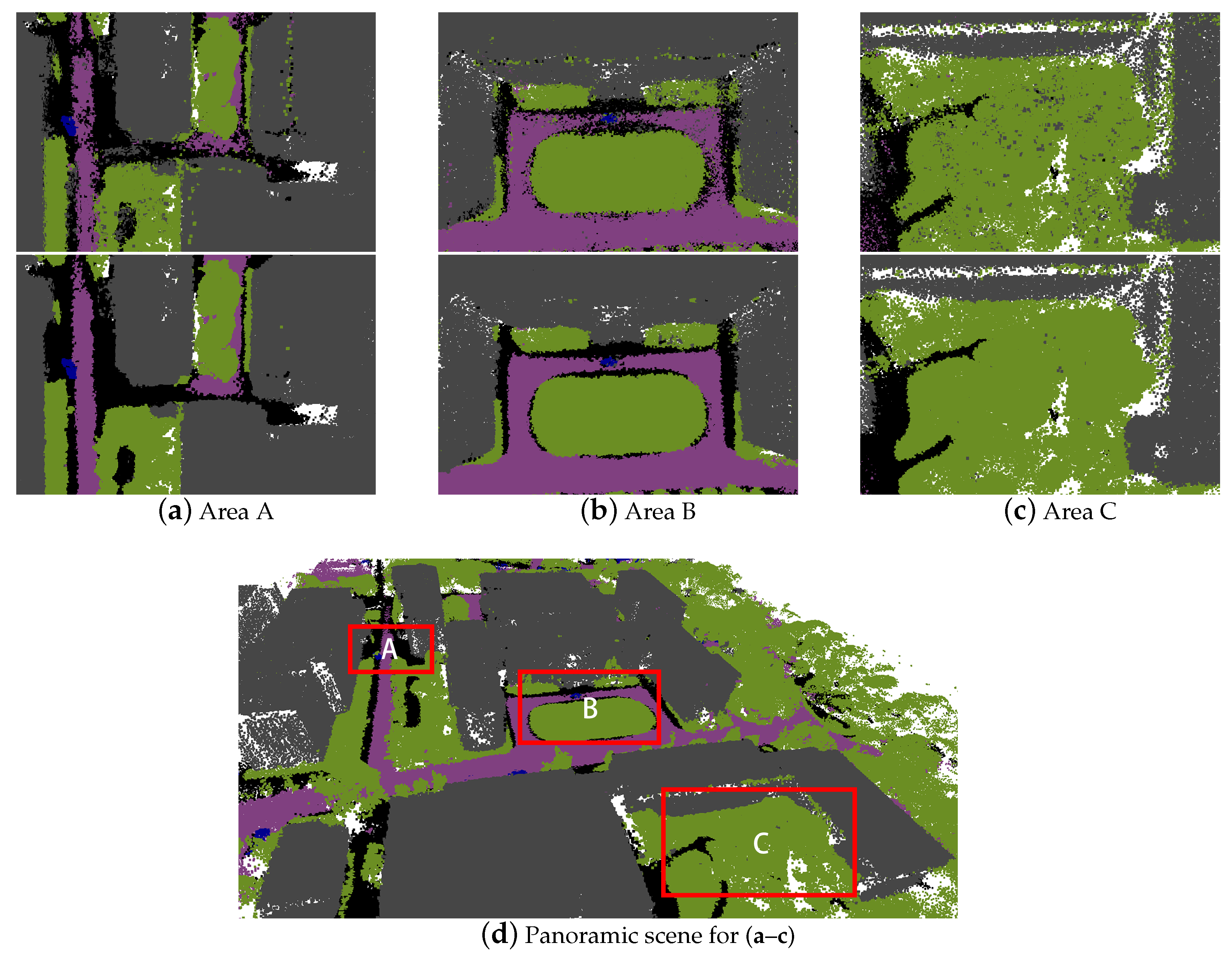
5. Results and Discussion

5.1. Quantitative Results

With the semantic fusion process introduced in Section 3.4, the coarse semantic 3D point cloud was generated. Its quantitative result is denoted as the 3D baseline in

Table 2. Quantitative results of different methods for semantic categories.

Pixel Accuracy(%)
Method	Building	Vegetation	Vehicle	Road	All
2D prediction	95.60	89.85	97.95	87.91	85.66
3D baseline	97.51	90.06	99.76	75.59	87.76
Local	96.20	91.38	99.74	68.61	88.24
Global	96.16	91.40	99.45	71.44	88.21
$Global+Local$	96.19	91.40	99.76	68.16	88.40
F1-Score(%)
Method	Building	Vegetation	Vehicle	Road
2D prediction	96.53	73.99	33.15	61.42
3D baseline	97.00	74.69	63.66	75.79
Local	97.13	74.87	62.72	75.63
Global	97.15	74.69	73.17	75.03
$Global+Local$	97.85	76.07	81.40	76.57

. To be more specific, most points in 3D baseline are correct, yet with outliers and errors. The evaluation result of 3D baseline’s re-projection map demonstrates that the 3D baseline is much better than 2D in both PA and F1-score. Figure 6a,b illustrate this fact vividly, where Vehicle is segmented badly in 2D segmentation and segmented much better in 3D baseline.

Furthermore, as shown in Table 2, the Pixel Accuracy of 3D baseline is 87.76%, and the F1-scores of Vehicle, Vegetation, and Road are relatively low. The refinement methods introduced in Section 3.5 are denoted as Local, Global, and Local+Global in Table 2. Local, Global, and Local+Global methods in Table 2 have been fully tested, and we put the best results under various parameters to this table. With refinement, the F1-score of Vehicle significantly rises, while Building, Vegetation, and Road also have increased scores. In addition, the Local+Global optimization approach is better than the Local or Global approach in each semantic category. It leads to the conclusion that the Local+Global approach outperforms any single Local or Global approach.

5.2. Discussion

In the following part, the discussion of our semantic fusion method will be arranged in three aspects: the down-sample rate, the parameter chosen for the k-nearest neighbor algorithm, and the decision strategies between soft and hard.

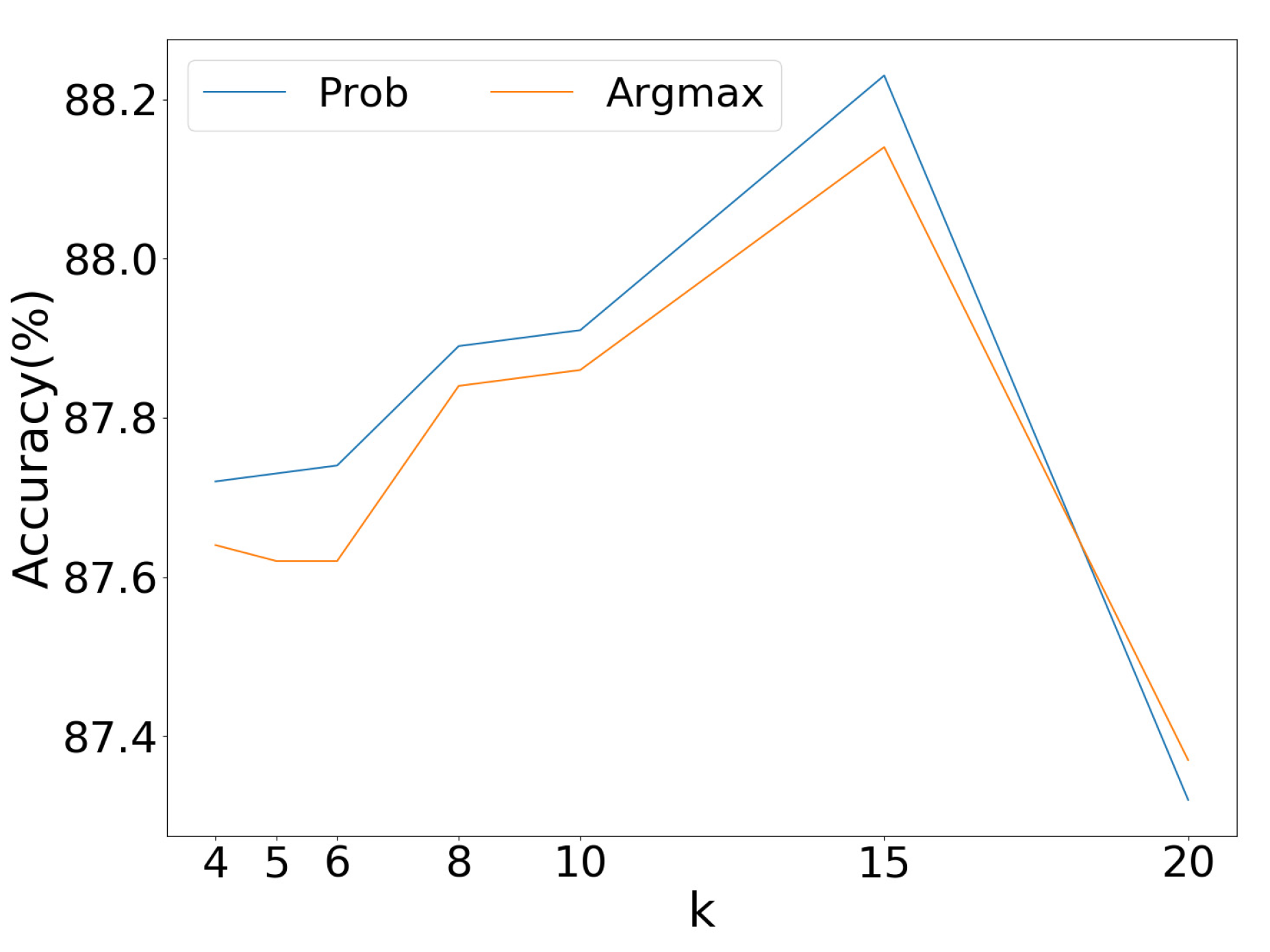
5.2.1. Parameter Selection for K-Nearest Neighbors

There are two criteria for judging neighbor points. As the name k-nearest neighbors itself indicates, the maximum number of neighbors is k. Besides that, the absolute distance in 3D space should also be limited. We down-sample the point could again with a rate of 0.001 to build a small KD-tree. Then we calculate the average distance of these points, setting the value to be the threshold of absolute distance. As indicated in Figure 7, the Pixel Accuracy firstly increases with the growth of k, and reaches its peak with $k=15$. After crossing the peak, accuracy decreases as k increases. This is because as k increases, the local method negatively optimizes for small areas such as vehicles and narrow roads.

5.2.2. Soft vs. Hard Decision Strategy

The decision strategies based on probability like Bayesian and Markov Decision are soft, while threshold and Argmax layer are hard decision strategies. There is no doubt that hard decision processes discard some information. As demonstrated in Figure 7, Prob outperforms Argmax under the same k in most circumstances. The best result of Prob is also greater than Argmax as well. It reveals that the soft decision strategy leads to better performance.

5.2.3. Down-Sample Rate

Since the dense point cloud’s scale of a specific outdoor scene collected by UAV is usually around 20M or bigger, global-wise algorithms cannot handle all points at once. For instance, PKU-M1 contains 27 million points.

Table 3. Ablation study on Down-sample rate.

Method	k-Nearest Neighbor	Down-Sample Rate	Pixel Accuracy(%)
2D prediction	0	1	85.66
3D baseline	0	0.1	87.76
Local	15	0.1	88.14
Local	15	0.2	88.02
Local	15	0.5	88.21
Local	15	1	88.24

shows a trend that the Pixel Accuracy generally reaches its peak at the down-sample rate of 1, equivalent to which means there are no down sampling process is taken at all. Increasing of down-sample rate makes the filtered point cloud denser, which intends the neighbors of a single point to become closer. The closer points are, the more likely they belong to the same semantic class. So it is sensible that the increasing of the down-sample rate avails the final Pixel Accuracy. If the performance of a method with lower sampling rate is higher than another, it is reasonable to believe that the former method is better.

6. Conclusions

In this paper, we proposed a semantic 3D reconstruction method to reconstruct 3D semantic models by integrating 2D semantic labeling and 3D geometric information. In implementation, we utilize deep learning for both 2D segmentation and depth estimation. Then, the semantic 3D point cloud is obtained by our probability-based semantic fusion method. Finally, we apply the local and global approaches for point cloud refinement. Experimental results show that our semantic fusing procedure with refinement based on local and global information is able to suppress noise and reduce the re-projection error. This work paves the way for realizing finer-grained 3D segmentation and semantic classifications.

References

1. Long, J.; Shelhamer, E.; Darrell, T. Fully convolutional networks for semantic segmentation. In Proceedings of the IEEE Conference on Computer Vision and Pattern Recognition, Boston, MA, USA, 7–12 June 2015; pp. 3431–3440. [Google Scholar]
2. Badrinarayanan, V.; Kendall, A.; Cipolla, R. Segnet: A deep convolutional encoder-decoder architecture for image segmentation. IEEE Trans. Pattern Anal. Mach. Intell. 2017, 39, 2481–2495. [Google Scholar] [CrossRef] [PubMed]
3. Chen, L.C.; Papandreou, G.; Kokkinos, I.; Murphy, K.; Yuille, A.L. Deeplab: Semantic image segmentation with deep convolutional nets, atrous convolution, and fully connected crfs. IEEE Trans. Pattern Anal. Mach. Intell. 2017, 40, 834–848. [Google Scholar] [CrossRef] [PubMed]
4. Zhao, H.; Shi, J.; Qi, X.; Wang, X.; Jia, J. Pyramid scene parsing network. In Proceedings of the IEEE Conference on Computer Vision and Pattern Recognition, Honolulu, HI, USA, 21–26 July 2017; pp. 2881–2890. [Google Scholar]
5. Yao, Y.; Luo, Z.; Li, S.; Fang, T.; Quan, L. Mvsnet: Depth inference for unstructured multi-view stereo. In Proceedings of the European Conference on Computer Vision (ECCV), Munich, Germany, 8–14 September 2018; pp. 767–783. [Google Scholar]
6. Yao, Y.; Luo, Z.; Li, S.; Shen, T.; Fang, T.; Quan, L. Recurrent mvsnet for high-resolution multi-view stereo depth inference. In Proceedings of the IEEE Conference on Computer Vision and Pattern Recognition, Long Beach, CA, USA, 16–20 June 2019; pp. 5525–5534. [Google Scholar]
7. Chen, Y.; Wang, Y.; Lu, P.; Chen, Y.; Wang, G. Large-scale structure from motion with semantic constraints of aerial images. In Proceedings of the Chinese Conference on Pattern Recognition and Computer Vision (PRCV), Guangzhou, China, 23–26 November 2018; pp. 347–359. [Google Scholar]
8. Bao, S.Y.; Savarese, S. Semantic structure from motion. In Proceedings of the CVPR 2011, Providence, RI, USA, 20–25 June 2011; pp. 2025–2032. [Google Scholar]
9. Martinovic, A.; Knopp, J.; Riemenschneider, H.; Van Gool, L. 3D all the way: Semantic segmentation of urban scenes from start to end in 3d. In Proceedings of the IEEE Conference on Computer Vision and Pattern Recognition, Santiago, Chile, 7–13 December 2015; pp. 4456–4465. [Google Scholar]
10. Wolf, D.; Prankl, J.; Vincze, M. Fast semantic segmentation of 3D point clouds using a dense CRF with learned parameters. In Proceedings of the 2015 IEEE International Conference on Robotics and Automation (ICRA), Seattle, WA, USA, 26–30 May 2015; pp. 4867–4873. [Google Scholar]
11. Häne, C.; Zach, C.; Cohen, A.; Pollefeys, M. Dense semantic 3d reconstruction. IEEE Trans. Pattern Anal. Mach. Intell. 2016, 39, 1730–1743. [Google Scholar] [CrossRef] [PubMed]
12. Hane, C.; Zach, C.; Cohen, A.; Angst, R.; Pollefeys, M. Joint 3D scene reconstruction and class segmentation. In Proceedings of the IEEE Conference on Computer Vision and Pattern Recognition, Portland, OR, USA, 23–28 June 2013; pp. 97–104. [Google Scholar]
13. Savinov, N.; Ladicky, L.; Hane, C.; Pollefeys, M. Discrete optimization of ray potentials for semantic 3d reconstruction. In Proceedings of the IEEE Conference on Computer Vision and Pattern Recognition, Santiago, Chile, 7–13 December 2015; pp. 5511–5518. [Google Scholar]
14. Wu, Z.; Song, S.; Khosla, A.; Yu, F.; Zhang, L.; Tang, X.; Xiao, J. 3d shapenets: A deep representation for volumetric shapes. In Proceedings of the IEEE Conference on Computer Vision and Pattern Recognition, Santiago, Chile, 7–13 December 2015; pp. 1912–1920. [Google Scholar]
15. Maturana, D.; Scherer, S. Voxnet: A 3d convolutional neural network for real-time object recognition. In Proceedings of the 2015 IEEE/RSJ International Conference on Intelligent Robots and Systems (IROS), Hamburg, Germany, 28 September–3 October 2015; pp. 922–928. [Google Scholar]
16. Qi, C.R.; Su, H.; Mo, K.; Guibas, L.J. Pointnet: Deep learning on point sets for 3d classification and segmentation. In Proceedings of the IEEE Conference on Computer Vision and Pattern Recognition, Honolulu, HI, USA, 21–26 July 2017; pp. 652–660. [Google Scholar]
17. Qi, C.R.; Yi, L.; Su, H.; Guibas, L.J. Pointnet++: Deep hierarchical feature learning on point sets in a metric space. In Proceedings of the Advances in Neural Information Processing Systems, Long Beach, CA, USA, 4–9 December 2017; pp. 5099–5108. [Google Scholar]
18. Vineet, V.; Miksik, O.; Lidegaard, M.; Nießner, M.; Golodetz, S.; Prisacariu, V.A.; Kähler, O.; Murray, D.W.; Izadi, S.; Pérez, P.; et al. Incremental dense semantic stereo fusion for large-scale semantic scene reconstruction. In Proceedings of the 2015 IEEE International Conference on Robotics and Automation (ICRA), Seattle, WA, USA, 26–30 May 2015; pp. 75–82. [Google Scholar]
19. Zhao, C.; Sun, L.; Stolkin, R. A fully end-to-end deep learning approach for real-time simultaneous 3D reconstruction and material recognition. In Proceedings of the 2017 18th International Conference on Advanced Robotics (ICAR), Hong Kong, China, 10–12 July 2017; pp. 75–82. [Google Scholar]
20. McCormac, J.; Handa, A.; Davison, A.; Leutenegger, S. Semanticfusion: Dense 3d semantic mapping with convolutional neural networks. In Proceedings of the 2017 IEEE International Conference on Robotics and Automation (ICRA), Singapore, Singapore, 29 May–3 June 2017; pp. 4628–4635. [Google Scholar]
21. Li, X.; Wang, D.; Ao, H.; Belaroussi, R.; Gruyer, D. Fast 3D Semantic Mapping in Road Scenes. Appl. Sci. 2019, 9, 631. [Google Scholar] [CrossRef] [Green Version]
22. Zhou, Y.; Shen, S.; Hu, Z. Fine-level semantic labeling of large-scale 3d model by active learning. In Proceedings of the 2018 International Conference on 3D Vision (3DV), Verona, Italy, 5–8 September 2018; pp. 523–532. [Google Scholar]
23. Stathopoulou, E.; Remondino, F. Semantic photogrammetry: boosting image-based 3D reconstruction with semantic labeling. Int. Arch. Photogramm. Remote Sens. Spat. Inf. Sci. 2019, 42, 2/W9. [Google Scholar] [CrossRef] [Green Version]
24. Zhang, R.; Li, G.; Li, M.; Wang, L. Fusion of images and point clouds for the semantic segmentation of large-scale 3D scenes based on deep learning. ISPRS J. Photogramm. Remote Sens. 2018, 143, 85–96. [Google Scholar] [CrossRef]
25. Schonberger, J.L.; Frahm, J.M. Structure-from-motion revisited. In Proceedings of the IEEE Conference on Computer Vision and Pattern Recognition, Las Vegas, NV, USA, 27–30 June 2016; pp. 4104–4113. [Google Scholar]
26. He, K.; Zhang, X.; Ren, S.; Sun, J. Deep residual learning for image recognition. In Proceedings of the IEEE Conference on Computer Vision and Pattern Recognition, Las Vegas, NV, USA, 27–30 June 2016; pp. 770–778. [Google Scholar]
27. Krizhevsky, A.; Sutskever, I.; Hinton, G.E. Imagenet classification with deep convolutional neural networks. In Proceedings of the Advances in Neural Information Processing Systems, Lake Tahoe, NV, USA, 3–8 December 2012; pp. 1097–1105. [Google Scholar]
28. Jensen, R.; Dahl, A.; Vogiatzis, G.; Tola, E.; Aanæs, H. Large scale multi-view stereopsis evaluation. In Proceedings of the IEEE Conference on Computer Vision and Pattern Recognition, Columbus, OH, USA, 23–28 June 2014; pp. 406–413. [Google Scholar]
29. Galliani, S.; Lasinger, K.; Schindler, K. Massively parallel multiview stereopsis by surface normal diffusion. In Proceedings of the IEEE International Conference on Computer Vision, Santiago, Chile, 7–13 December 2015; pp. 873–881. [Google Scholar]
30. Sedlacek, D.; Zara, J. Graph cut based point-cloud segmentation for polygonal reconstruction. In Proceedings of the International Symposium on Visual Computing, Las Vegas, NV, USA, 30 November–2 December 2009; pp. 218–227. [Google Scholar]
31. Boykov, Y.; Kolmogorov, V. An experimental comparison of min-cut/max-flow algorithms for energy minimization in vision. IEEE Trans. Pattern Anal. Mach. Intell. 2004, 26, 1124–1137. [Google Scholar] [CrossRef] [PubMed] [Green Version]
32. Cordts, M.; Omran, M.; Ramos, S.; Rehfeld, T.; Enzweiler, M.; Benenson, R.; Franke, U.; Roth, S.; Schiele, B. The cityscapes dataset for semantic urban scene understanding. In Proceedings of the IEEE Conference on Computer Vision and Pattern Recognition, Las Vegas, NV, USA, 27–30 June 2016; pp. 3213–3223. [Google Scholar]
33. Abadi, M.; Agarwal, A.; Barham, P.; Brevdo, E.; Chen, Z.; Citro, C.; Corrado, G.S.; Davis, A.; Dean, J.; Devin, M.; et al. TensorFlow: Large-scale machine learning on heterogeneous systems. arXiv 2015, arXiv:1603.04467. [Google Scholar]
34. Bottou, L. Large-scale machine learning with stochastic gradient descent. In Proceedings of COMPSTAT’2010; Springer: Paris, France, 2010; pp. 177–186. [Google Scholar]
Figure 1. General pipeline of our work. Three branches are implemented to process the reconstruction dataset. The upper branch is the semantic segmentation branch to predict the semantic probability map; the middle branch is SfM to calculate the 3D odometry and camera poses; the lower branch is to estimate the depth map. Then, semantic fusion is applied to fuse them into a coarse point cloud. The last step is to refine the point cloud by local and global methods.
Applsci 10 01275 g001
Figure 2. Visualization of the depth map estimated by the learning-based MVS method. (a) The input image. (b) Depth estimation by R-MVSNet [6]. (c) Refined depth by bilateral filtering.
Applsci 10 01275 g002
Figure 3. Illustration of our semantic fusion method: the 3D semantic labels are determined by multi-view information; the 3D point’s label is decided by the correspondence accumulated probability of 2D pixels in each image.
Applsci 10 01275 g003
Figure 4. Comparison between the point clouds before and after refinement. (ac) Top: coarse result. Bottom: refined result. (d): The panoramic scene for (ac).
Applsci 10 01275 g004
Figure 5. Visualization of PKU-M1.(a): A sample image of PKU-M1, (b): ground truth of (a), (c): prediction of (a), and (d): 3D re-projection map of (a). Since the re-projection map (d) is quite sparse, we use Pixel Accuracy to compare the re-projection map and the ground truth map. Grey: Building, Green: Vegetation, Blue: Vehicle, Pink: Road, Black: Background. Best viewed in color.
Applsci 10 01275 g005
Figure 6. (a) is the Confusion Matrix for 2D segmentation, (b) is the Confusion Matrix for re-projection images. Four categories are evaluated, which are Building, Vegetation, Road and Vehicle. It shows that the re-projection map from 3D semantic points behaves higher accuracy compared with 2D segmentation, due to considering multi-view information.
Applsci 10 01275 g006
Figure 7. Ablation study on parameter selection for k-nearest neighbor and soft vs. hard decision strategy. For both Prob and Argmax methods, k = 15 is the best parameter. In most circumstances, the soft decision strategy Prob dominates hard decision strategy Argmax.
Applsci 10 01275 g007