Accurate BAPL Score Classification of Brain PET Images Based on Convolutional Neural Networks with a Joint Discriminative Loss Function † †


Abstract
:1. Introduction
2. Materials
3. Methods
3.1. FBB PET Interpretations
3.2. CNN Models
3.2.1. VGG19
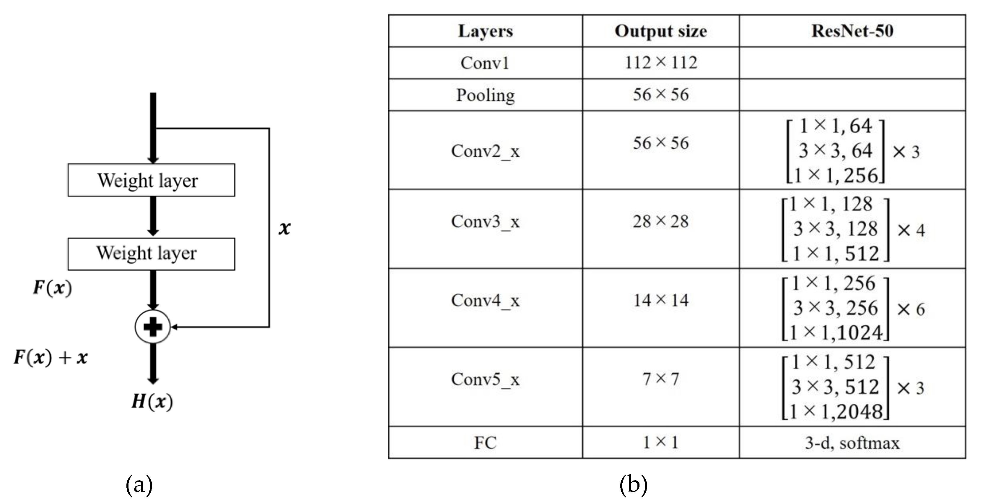
3.2.2. ResNet50
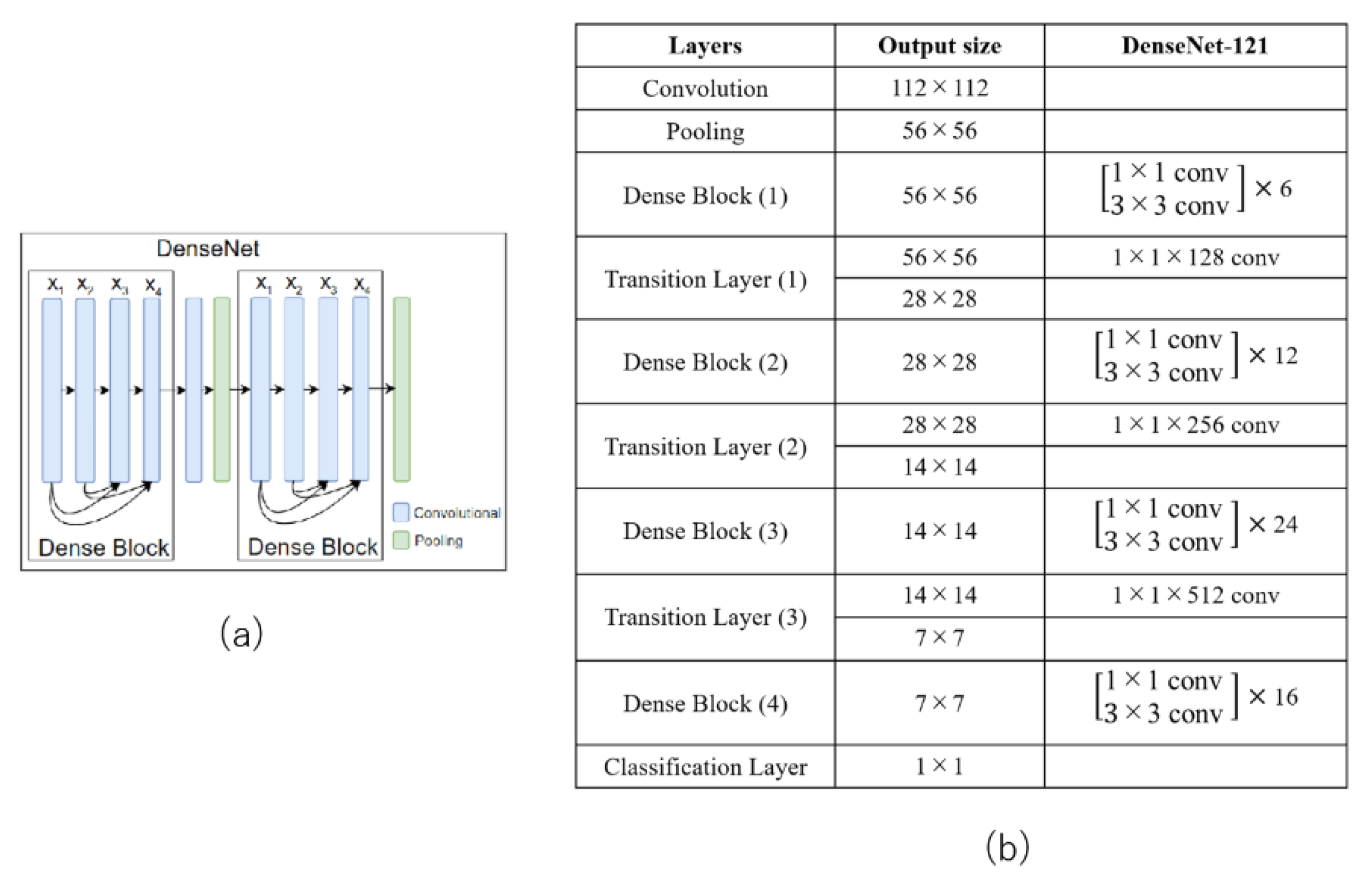
3.2.3. DenseNet121
3.3. Joint Loss Function
3.4. Data Augmentation with Mix-Up
4. Results and Discussion
4.1. Experimental Setup
4.2. Effectiveness of Data Augmentation Based on Mix-up
4.3. Impact of λ
4.4. Coronal Plane versus Axial Plane
4.5. Detailed Comparison between the Proposed and Conventional Loss Functions on Three Network Architectures
4.6. Two-Class Classification
4.7. Data Visualization and Discussion
5. Conclusions
Author Contributions
Funding
Conflicts of Interest
References
- World Alzheimer Report. Available online: https://www.alz.co.uk/research/WorldAlzheimerReport2015.pdf (accessed on 13 November 2019).
- Cheng, D.; Liu, M. Combining Convolutional and Recurrent Neural Networks for Alzheimer’s Disease Diagnosis Using PET Images. In Proceedings of the 2017 IEEE International Conference on Imaging Systems and Techniques, Beijing, China, 18–20 October 2017. [Google Scholar]
- Plant, C.; Teipel, S.J.; Oswald, A.; Böhm, C.; Meindl, T.; Mourao-Miranda, J.; Bokde, A.W.; Hampel, H.; Ewers, M. Automated detection of brain atrophy patterns based on MRI for the prediction of Alzheimer’s disease. Neuroimage 2010, 50, 162–174. [Google Scholar] [CrossRef] [PubMed] [Green Version]
- Dubois, B.; Feldman, H.H.; Jacova, C.; Hampel, H.; Molinuevo, J.L.; Blennow, K.; DeKosky, S.T.; Gauthier, S.; Selkoe, D.; Bateman, R.; et al. Advancing research diagnostic criteria for Alzheimer’s disease: The IWG-2 criteria. Lancet Neurol. 2014, 13, 614–629. [Google Scholar] [CrossRef]
- Pillai, J.A.; Cummings, J.L. Clinical trials in predementia stages of Alzheimer disease. Med. Clin. N. Am. 2013, 97, 439–457. [Google Scholar] [CrossRef] [PubMed]
- Jack, C.R.; Knopman, D.S.; Jagust, W.J.; Petersen, R.C.; Weiner, M.W.; Aisen, P.S.; Shaw, L.M.; Vemuri, P.; Wiste, H.J.; Weigand, S.D.; et al. Tracking pathophysiological processes in Alzheimer’s disease: An updated hypothetical model of dynamic biomarkers. Lancet Neurol. 2013, 12, 207–216. [Google Scholar] [CrossRef] [Green Version]
- Choi, H.; Jin, K.H. Predicting cognitive decline with deep learning of brain metabolism and amyloid imaging. Behav. Brain Res. 2018, 344, 103–109. [Google Scholar] [CrossRef] [PubMed] [Green Version]
- Barthel, H.; Gertz, H.J.; Dresel, S.; Peters, O.; Bartenstein, P.; Buerger, K.; Hiemeyer, F.; Wittemer-Rump, S.M.; Seibyl, J.; Reininger, C.; et al. Cerebral amyloid-β PET with florbetaben (18F) in patients with Alzheimer’s disease and healthy controls: A multicentre phase 2 diagnostic study. Lancet Neurol. 2011, 10, 424–435. [Google Scholar] [CrossRef]
- Zhang, D.; Wang, Y.; Zhou, L.; Yuan, H.; Shen, D. Multimodel classification of Alzheimer’s disease and mild cognitive impairment. NeuroImage 2011, 55, 856–867. [Google Scholar] [CrossRef] [PubMed] [Green Version]
- Sarraf, S.; Tofighi, G. DeepAD: Alzheimer’s disease classification via deep convolutional neural networks using MRI and fMRI. bioRxiv 2016. [Google Scholar] [CrossRef] [Green Version]
- Farooq, A.; Anwar, S.; Muhammad Awais, M.; Saad Rehman, S. A Deep CNN based Multi-class Classification of Alzheimer’s Disease Using MRI. In Proceedings of the IEEE Instrumentation and Measurement, Beijing, China, 18–20 October 2017. [Google Scholar]
- Kang, H.; Kim, W.G.; Yang, G.S.; Kim, H.W.; Jeong, J.E.; Yoon, H.J.; Cho, K.; Jeong, Y.J.; Kang, D.Y. VGG-based BAPL Score Classification of 18F-Florbetaben Amyloid Brain PET. Biomed. Sci. Lett. 2018, 24, 418–425. [Google Scholar] [CrossRef]
- Liu, M.; Cheng, D.; Yan, W. Classification of Alzheimer’s Disease by Combination of Convolutional and Recurrent Neural Networks Using FDG-PET Images. Front. Neuroinform. 2018, 12, 35. [Google Scholar] [CrossRef] [PubMed] [Green Version]
- Zhang, H.; Cissé, M.; Lopez-Paz, D. Mix-Up: Beyond Empirical Risk Minimization. In Proceedings of the International Conference on Learning Representations (ICLR), Vancouver, BC, Canada, 30 April–3 May 2018. [Google Scholar]
- Friston, K.J.; Ashburner, J.; Frith, C.D.; Poline, J.B.; Heather, J.D.; Frackowiak, R.S.J. Spatial registration and normalization of images. Hum. Brain Map. 1995, 3, 165–189. [Google Scholar] [CrossRef]
- Sato, R.; Iwamoto, Y.; Cho, K.; Kang, D.Y.; Chen, Y.W. Comparison of CNN Models with Different Plane Images and Their Combinations for Classification of Alzheimer’s Disease Using PET Images. In Innovation in Medicine and Healthcare Systems, and Multimedia; Chen, Y.W., Zimmermann, A., Howlett, R., Jain, L., Eds.; Smart Innovation, Systems and Technologies (Proc. of InMed2019); Springer: St. Julians, Malta, 2019; Volume 145, pp. 169–177. [Google Scholar]
- Simonyan, K.; Zisserman, A. Very Deep Convolutional Networks for Large-Scale Image Recognition. In Proceedings of the International Conference on Learning Representations (ICLR), Sandiego, CA, USA, 7–9 May 2015. [Google Scholar]
- He, K.; Zhang, X.; Ren, S.; Sun, J. Deep residual learning for image recognition. arXiv 2015, arXiv:1512.03385. [Google Scholar]
- Huang, G.; Liu, Z.; van der Maaten, L.; Weinberger, K.Q. Densely connected convolutional networks. In Proceedings of the IEEE Conference on Computer Vision and Pattern Recognition (CVPR), Honolulu, HI, USA, 21–26 July 2017; pp. 1097–1105. [Google Scholar]
- Liang, D.; Lin, L.; Hu, H.; Zhang, Q. Combining Convolutional and Recurrent Neural Networks for Classification of Focal Liver Lesions in Multi-Phase CT Images. In MICCAI 2018, LNCS 11071; Frangi, A.F., Schnabel, J.A., Davatzikos, C., Alberola-López, C., Fichtinger, G., Eds.; Springer: Cham, Switzerland, 2018; pp. 666–675. [Google Scholar]
- Wen, Y.; Zhang, K.; Li, Z.; Qiao, Y. A discriminative feature learning approach for deep face recognition. In ECCV2016, LNCS; Leibe, B., Matas, J., Sebe, N., Welling, M., Eds.; Springer: Cham, Switzerland, 2016; Volume 9911, pp. 499–515. [Google Scholar]
- Chollet, F.; Rahman, F.; Lee, T.; Marmiesse, G.; Zabluda, O.; Pumperla, M.; Santana, E.; McColgan, T.; Snelgrove, X.; Branchaud-Charron, F.; et al. Keras: The Python Deep Learning Library. 2015. Available online: https://keras.io (accessed on 13 November 2019).
- Abadi, M.; Agarwal, A.; Barham, P.; Brevdo, E. Tensorflow: Large-scale machine learning on heterogeneous distributed systems. arXiv 2016, arXiv:1603.04467. [Google Scholar]
- Deng, J.; Dong, W.; Socher, R.; Li, L.J.; Li, K.; Li, F.F. Imagenet: A large-scale hierarchical image database. In Proceedings of the IEEE Conference on Computer Vision and Pattern Recognition, Miami, FL, USA, 20–25 June 2009. [Google Scholar]
- Center Loss Implementation in Keras. Available online: https://github.com/handongfeng/MNIST-center-loss (accessed on 13 November 2019).
- Payan, A.; Montana, G. Predicting Alzheimer’s Disease: A Neuroimaging Study with 3D Convolutional Neural Networks. arXiv 2015, arXiv:1502.02506. [Google Scholar]


| Diagnosis | Number | Age | Gender (F/M) |
|---|---|---|---|
| BAPL1 | 188 | 67.1 ± 8.7 | 71/117 |
| BAPL2 | 48 | 72.8 ± 6.1 | 21/27 |
| BAPL3 | 144 | 69.3 ± 7.9 | 62/82 |
| Train | Test | |
|---|---|---|
| BAPL1 | 165 subject (1,815→5,445 slices) | 23 subjects (253 slices) |
| BAPL2 | 42 subjects (462→4620 slices) | 6 subjects (66 slices) |
| BAPL3 | 126 subjects (1386→4,620 slices) | 18 subjects (198 slices) |
| Total | 15,609 slices | 517 slices |
| Without Data Aaugmentation | With Data Aaugmentation | |
|---|---|---|
| Translation and Inversion | Mixup | |
| 83.87% | 86.13% | 88.90% |
| λ | 0 | 0.001 | 0.0025 | 0.005 | 0.01 | 0.1 |
| Accuaracy | 88.90% | 89.53% | 91.03% | 90.12% | 89.32% | 89.53% |
| Plane for Analysis | Accuracy | Accuracy per Case |
|---|---|---|
| Axial Plane | 85.18% | 87.50% |
| Coronal Plane | 91.03% | 93.75% |
| Method | Precison | Recall | F1 Score | Accuracy | ||
|---|---|---|---|---|---|---|
| VGG19 | λ = 0 | BAPL1 | 88.16% | 91.60% | 89.85% | 81.50% |
| BAPL2 | 40.25% | 17.50% | 24.39% | |||
| BAPL3 | 78.52% | 89.40% | 83.61% | |||
| λ = 0.0025 | BAPL1 | 87.96% | 93.20% | 90.50% | 88.60% | |
| BAPL2 | 100% | 51.50% | 67.99% | |||
| BAPL3 | 87.51% | 94.90% | 91.06% | |||
| ResNet50 | λ = 0 | BAPL1 | 92% | 92.60% | 92.40% | 88.90% |
| BAPL2 | 73.70% | 40.20% | 52.02% | |||
| BAPL3 | 81.90% | 94.10% | 87.58% | |||
| λ = 0.0025 | BAPL1 | 93.63% | 92.00% | 92.81% | 91.03% | |
| BAPL2 | 67.80% | 62.10% | 64.82% | |||
| BAPL3 | 89.80% | 92.00% | 90.89% | |||
| DenseNet121 | λ = 0 | BAPL1 | 97.38% | 88.30% | 92.62% | 88.06% |
| BAPL2 | 67.79% | 53.00% | 59.49% | |||
| BAPL3 | 89.76% | 99.40% | 94.33% | |||
| λ = 0.0025 | BAPL1 | 100% | 97.70% | 98.84% | 94.86% | |
| BAPL2 | 85.32% | 72.70% | 78.51% | |||
| BAPL3 | 91.57% | 98.90% | 95.09% | |||
| Method | BAPL1 versus (BAPL2 + BAPL3) | (BAPL1 + BAPL2) versus BAPL3 |
|---|---|---|
| λ = 0 | 90.91% | 92.42% |
| λ = 0.0025 | 96.97% | 95.55% |
© 2020 by the authors. Licensee MDPI, Basel, Switzerland. This article is an open access article distributed under the terms and conditions of the Creative Commons Attribution (CC BY) license (http://creativecommons.org/licenses/by/4.0/).
Share and Cite
Sato, R.; Iwamoto, Y.; Cho, K.; Kang, D.-Y.; Chen, Y.-W. Accurate BAPL Score Classification of Brain PET Images Based on Convolutional Neural Networks with a Joint Discriminative Loss Function †. Appl. Sci. 2020, 10, 965. https://doi.org/10.3390/app10030965
Sato R, Iwamoto Y, Cho K, Kang D-Y, Chen Y-W. Accurate BAPL Score Classification of Brain PET Images Based on Convolutional Neural Networks with a Joint Discriminative Loss Function †. Applied Sciences. 2020; 10(3):965. https://doi.org/10.3390/app10030965
Chicago/Turabian StyleSato, Ryosuke, Yutaro Iwamoto, Kook Cho, Do-Young Kang, and Yen-Wei Chen. 2020. "Accurate BAPL Score Classification of Brain PET Images Based on Convolutional Neural Networks with a Joint Discriminative Loss Function †" Applied Sciences 10, no. 3: 965. https://doi.org/10.3390/app10030965