Prediction of Driver’s Attention Points Based on Attention Model

Featured Application

The method proposed in our paper is mainly applied in the intelligent driving fields. At present, our method can filter out useless information that is captured by vision sensors and reduce the complexity of visual information processing in the intelligent driving fields. In the future, our method can establish the relationship between the driver’s regions of interest and the driving behaviors. The driver’s regions of interest are used as the input and the driving behaviors are used as the output to realize unmanned driving. This solution can effectively reduce the cost of unmanned driving, because a large number of sensors, like radar, are not needed.

Abstract

The current intelligent driving system does not consider the selective attention mechanism of drivers, and it cannot completely replace the drivers to extract effective road information. A Driver Visual Attention Network (DVAN), which is based on deep learning attention model, is proposed in our paper, in order to solve this problem. The DVAN is aimed at extracting the key information affecting the driver’s operation by predicting the driver’s attention points. It completes the fast localization and extraction of road information that is most interesting to drivers by merging local apparent features and contextual visual information. Meanwhile, a Cross Convolutional Neural Network (C-CNN) is proposed in order to ensure the integrity of the extracted information. Here, we verify the network on the KITTI dataset, which is the largest computer vision algorithm evaluation data set in the world’s largest autonomous driving scenario. Our results show that the DVAN can quickly locate and identify the target that the driver is most interested in a picture, and the average accuracy of prediction is 96.3%. This will provide useful theoretical basis and technical methods that are related to visual perception for intelligent driving vehicles, driving training and assisted driving systems in the future.

1. Introduction

In recent years, many society and livelihood issues, such as traffic safety, congestion, pollution, and energy consumption are accompanied with the continuous increase of car ownership and traffic flow. According to statistics, more than 94% of traffic accidents are related to the driver’s behaviors [1], and the driver’s distracted behaviors will affect his operating behaviors, thereby inducing a traffic accident. Additionally, the driver’s perceptions of danger greatly affect the driver’s driving behaviors.

Many scholars carry out research from multiple aspects, such as supervision on fatigue driving [2,3], prediction of traffic flow [4] and so on, in order to reduce the occurrence of traffic accidents. Meanwhile intelligent driving systems are also being widely used. The current detection of road target information in intelligent driving systems mainly uses the method of combining the target detection algorithm that is based on deep learning and hardware, such as radar. Firstly, all of the road target information is identified by the vision sensor while using the target detection algorithm, and then static or dynamic objects can be identified, detected, and tracked by using radar or infrared technology, thereby taking corresponding measures. At present, the target detection algorithms that are based on deep learning are mainly divided into two categories, one of which is based on the region proposal framework, and the other is based on regression/classification framework [5].

The target detection algorithm that is based on the regional proposal framework is based on the R-CNN target detection model that was proposed by Ross GirShick and others in 2014 [6], and uses the idea of this model to propose a large number of better target detection models. The target detection algorithm that is based on the regional proposal framework uses the idea of R-CNN proposed by Ross GirShick et al. in 2014, and many scholars have proposed a series of better target detection models. The most representative of them is the Faster R-CNN model that was proposed by Ren Shaoqing et al. [7]. This model greatly improving the detection speed of model. However, limited by the calculation of a large number of candidate regions, there is still a large gap between the model and the real-time detection. For the slow speed, problems, such as R-CNN and Faster R-CNN, the target detection algorithm that is based on the regression/classification framework directly implements the mapping from image pixels to bounding box coordinates and object class probability. This greatly improves the detection speed of the algorithm, but it is slightly inferior in detection accuracy. Its representatives are YOLO and SSD.

In 2016, Redmond et al. [8] proposed Yolo, which follows the design concept of end-to-end training and real-time detection. Soon after, Redmond et al. designed Darknet-19 based on Yolo and proposed Yolov2 [9] while using batch normalization [10]. In 2018, Redmond drew ideas from ResNet [11] and Feature Pyramid Networks (FPN) [12] algorithm, and proposed Yolov3 [13], thus greatly improving the detection accuracy. Much of the target detection in the field of intelligent driving is based on Yolo. Putra M H et al. [14] realized a real-time human-car detector by improving Yolo. Yang W et al. [15] proposed a real-time vehicle detection method that was based on Yolov2, which can complete vehicle detection and realize vehicle classification in real time.

When compared with Yolo, the Single Shot MultiBox Detector (SSD) that was proposed by Liu Wei et al. [16] has three differences. The first is that SSD uses the Convolutional Neural Network (CNN) to detect directly, instead of detecting after the fully connected layer, like Yolo. Secondly, SSD extracts feature graphs of different scales for detection. The large scale feature graph (the earlier feature graph) can be used to detect small objects, while the small scale feature graph (the later feature graph) is used to detect large objects. Thirdly, SSD adopts prior frames with different dimensions and aspect ratios. Kim H et al. [17] proposed a target detection model in the road driving environment, which was migrated from SSD on KITTI data set.

To sum up, although the two types of target detection algorithms in the field of intelligent driving currently have their own advantages in detection accuracy and speed, they are both universal target detection algorithms, that is, they will recognize all information that is captured by the visual sensors. However, it is obviously unnecessary to detect objects, such as distant trees, buildings, and even vehicles that are separated by several lanes. It is more efficient to directly detect dangerous targets or regions in front of the road and only extract the target information in the image that affects the car’s driving process, ignoring many unnecessary details.

In recent years, there have been few studies on the driver’s region of interest based on real traffic scenes. Andrea Palazzi et al. [18] produced a video dataset of traffic scenes that can be used for predicting the driver’s attention position, named DR (eye) VE. The DR (eye) VE contains 74 segments of 5-min. traffic driving videos, which respectively record the eye movement data of eight drivers during real driving, and each only video contains one driver’s eye movement data information. In subsequent work, they used different computer vision models to train on their data set to predict the driver’s attention [19,20]. Tawari and Kang [21] further improved the focus prediction results on the DR (eye) VE database through Bayesian theory.

The data set contains a total of 550,000 frames of video images, and also records GPS, vehicle speed, and other information. For the study of the driver’s visual attention mechanism in the driving scenes, the eye movement data in each video only contains a single driver, which might cause some images that are related to traffic driving to be lost due to the individual differences of the driver information. In addition, the driver reads external information in a chronological order during driving, instead of acquiring information from a single picture. Using this data set ignores the effect of chronological order on the driver’s visual attention mechanism.

We build the DVAN based on the attention model in order to simulate the driver’s visual attention mechanism. The attention model was originally used for text translation, but it is now gradually applied to the field of intelligent driving. Jaderberg et al. [22] believe that pooling operation will lead to unrecognized or lost key information. Therefore, a spatial domain attention model was proposed in 2015, in which the spatial transformer performed corresponding spatial transformation on the spatial domain information in the picture to extract the key information. In 2017, HuJie et al. [23] proposed a channel domain attention model, which added weight to the signals on each channel. Different weight values represent different degrees of importance of information. The larger the weight, the higher the importance of the information. In 2017, Wang Fei et al. [24] effectively combined the attention models of spatial domain and channel domain to form a mixed domain attention model for feature extraction. However, the above attention model can only process a single picture. The driver’s visual attention mechanism processes external information in a chronological order, and rich contextual information is very important [25]. Mnih, Volodymy et al., combined with the Recurrent Neural Network (RNN), proposed the Recurrence Attention Model [26] in order to extract the key information from the input with time sequence features, but this model is prone to gradient attenuation or explosion when capturing the dependency relation with large time step distance in the time sequence.

Our method improves the Recurrence Attention Model and builds a driver’s visual attention network based on it, which was used to simulate the driver’s visual attention mechanism. Finally, we analyze the prediction results through the KITTI data set.

2. Driver Visual Attention Network

We propose a driver’s visual attention network (DVAN) based on deep learning attention model in order to simulate the driver’s visual attention mechanism, predict the driver’s attention points, and achieve efficient extraction of key road information. The network mainly includes Visual Information Extraction Module (VEM), Information Processing Module (IPM), and Multi-tasking Output Module (MOM). Figure 1 shows the overall structure.

2.1. Visual Information Extraction Module (VEM)

The VEM acts as a driver’s eye for effectively extracting the road information of interest. The driver needs to search for and quickly locate the target or region of interest during driving. The rich contextual information provides effective information source [27], which enables the driver to quickly guide his attention and eyes to the region of interest in the road. VEM employs Information Capture (IC) combined with Cross Convolutional Neural Network (C-CNN) to extract the features from the driver’s regions of interest containing rich contextual information.

Information Capture (IC): The IC is used to simulate the driver’s retina to extract valid road information. As shown in Figure 2, the red region represents the region of interest to the driver. IC extracts several image blocks ${\mathrm{I}}_{\mathrm{i}}^{\mathrm{t}}$ (i = 1,2,3,…,n) of different scales from the whole input image I centering on the given attention point ${\mathrm{P}}^{\mathrm{t}}$ during the t–1 cycle. The image blocks ${\mathrm{I}}_{\mathrm{i}}^{\mathrm{t}}$ (i = 1,2,3,…,n) parameter is q, minimum scale is ${\mathrm{S}}_{\mathrm{m}}$, scale factor is set to ${\mathrm{s}}_{\mathrm{f}}$, and the number of scales is n. Subsequently, the size of the NO.i image block extracted by the IC is ${\mathrm{S}}_{\mathrm{i}}={\mathrm{S}}_{\mathrm{m}}\times {\mathrm{s}}_{\mathrm{f}}^{\mathrm{i}-1}$, and then adjusts all image blocks to uniform size ${\mathrm{S}}_{\mathrm{u}}$. Its mathematical mapping (${\varnothing }^{\mathrm{E}}$) is expressed as:

$$\left\{{\mathrm{I}}_{\mathrm{i}}^{\mathrm{t}}\right\}={\varnothing }^{\mathrm{E}}\left(\mathrm{I},{\mathrm{s}}_{\mathrm{f}},\mathrm{q}\right),\mathrm{i}=1,2, 3,\dots ,\mathrm{n}$$

(1)

Cross Convolutional Neural Network (C-CNN): We propose the C-CNN in order to ensure the integrity of the information of the image block ${\mathrm{I}}_{\mathrm{i}}^{\mathrm{t}}$ (i = 1, 2, 3, …, n) extracted from IC, which is shown in Figure 3. The effective road information captured by IC is retained to the greatest extent through the C-CNN and the reduction of pooling operation.

The C-CNN consists of five convolution layers ${\mathsf{\mu }}^{\mathsf{\sigma }}$ with parameters $\mathsf{\phi }$, one pooling layer and one full connection layer with parameters ${\mathrm{W}}_{\mathrm{f}}^{\mathrm{c}}$ and ${\mathrm{B}}_{\mathrm{f}}^{\mathrm{c}}$, where in the convolution layer includes convolution operation and ReLU activation function. Make the output of $\mathrm{CONV}\left(\mathrm{k}\right)$ be C (k) (k = 1, 2, 3, 4, 5). In C-CNN, the input of $\mathrm{CONV}\left(1\right)$ is the image block ${\mathrm{X}}_{\mathrm{i} }^{\mathrm{t}}$ with size ${\mathrm{S}}_{\mathrm{u}}$ being extracted by IC, the inputs of $\mathrm{CONV}\left(2\right)$, $\mathrm{CONV}\left(3\right)$, $\mathrm{CONV}\left(4\right)$, and $\mathrm{CONV}\left(5\right)$ are C1, C2, C1 + C3, and C2 + C4, respectively. Finally, C5 passes through the maximum pooling layer and the full connection layer to obtain the output ${\mathrm{Y}}_{\mathrm{i}}^{\mathrm{t}}$, whose expression is shown in Formula (2).

$${\mathrm{Y}}_{\mathrm{i}}=\max \left\{{\mathrm{W}}_{\mathrm{f}}^{\mathrm{c}}\left({\complement }^{\partial }{\mathsf{\mu }}^{\mathsf{\sigma }}\left({\mathrm{maI}}_{\mathrm{i}}^{\mathrm{t}}\right)\right)+{\mathrm{B}}_{\mathrm{f}}^{\mathrm{c}}, 0\right\}$$

(2)

2.2. Information Processing Module (IPM)

The Information Processing Module (IPM) plays the role of the driver’s brain, performs fusion processing on various information, and outputs the final instruction to the Multi-tasking Output Module (MOM). The IPM aims to merge the information ${\mathrm{Y}}_{\mathrm{i}}^{\mathrm{t}}$ (i = 1, 2, 3,…, n) output by each C-CNN in the VEM at time t with the information output by the attention point ${\mathrm{P}}^{\mathrm{t}}$ through the full connection layer. The Gate Recurrent Unit (GRU) processed the merged information, and finally the output ${\mathrm{H}}_{\mathrm{t}}^{\mathrm{l}}$ is obtained.

For each image block ${\mathrm{I}}_{\mathrm{i}}^{\mathrm{t}}$ (i = 1, 2, 3,…, n) extracted by the IC in the t cycle, the C-CNN will perform feature extraction on it to obtain ${\mathrm{Y}}_{\mathrm{i}}^{\mathrm{t}}$ (i = 1, 2, 3,…, n). Subsequently, combine multiple features together to obtain ${\mathrm{Y}}_{\mathrm{S}}^{\mathrm{t}}$. At the same time, attention point ${\mathrm{P}}^{\mathrm{t}}$ is mapped into the eigenvector ${\mathrm{X}}_{\mathrm{p}}^{\mathrm{t}}$ of the same dimension as ${\mathrm{Y}}_{\mathrm{S}}^{\mathrm{t}}$ through the full connection layer, and then ${\mathrm{Y}}_{\mathrm{S}}^{\mathrm{t}}$ and ${\mathrm{X}}_{\mathrm{p}}^{\mathrm{t}}$ are spliced (${\complement }^{\partial }$) to feature merger, the merged feature ${\mathrm{E}}^{\mathrm{t}}$ can be expressed by Equation (3).

$${\mathrm{E}}^{\mathrm{t}}={\mathrm{C}}^{\partial }\left({\mathrm{Y}}_{\mathrm{S}}^{\mathrm{t}},{\mathrm{X}}_{\mathrm{p}}^{\mathrm{t}}\right)$$

(3)

The Recurrence Attention Model uses RNN to process the time series information. However, the RNN is prone to gradient attenuation and gradient explosion when capturing the large number of time steps in the time series. We adopted GRU [28] instead of RNN in order to solve this problem. GRU is a kind of RNN and a very effective variant of Long-Short Term Memory (LSTM) [29]. When compared with the LSTM network, GRU is simpler in structure and has fewer parameters. It can effectively deal with the problem that RNN is difficult to capture the dependency of time step distance in time series due to gradient attenuation and gradient explosion. Therefore, our method selects three layers of GRU to process the characteristic information ${\mathrm{E}}^{\mathrm{t}}$ with time series, and takes the hidden state ${\mathrm{H}}_{\mathrm{t}}^{\mathrm{l}}$ of the last layer of GRU as the final output of the entire GRU mapping. Figure 4 shows the GRU structure.

The input of reset gate (${\mathrm{R}}^{\mathrm{t}}$) and update gate (${\mathrm{Z}}^{\mathrm{t}}$) are both time step input ${\mathrm{E}}^{\mathrm{t}}$ at time t and hidden state ${\mathrm{H}}_{\mathrm{t}-1}$ at the previous time. The output is calculated by full connection layer (σ), with sigmoid as activation function to ensure the output values ${\mathrm{R}}^{\mathrm{t}}$, ${\mathrm{Z}}^{\mathrm{t}}$ ∈ [0,1]. Reset gate (${\mathrm{R}}^{\mathrm{t}}$) helps to capture short-term dependencies in time series, and ${\mathrm{Z}}^{\mathrm{t}}$ helps to capture long-term dependencies in time series. Formula (4) shows the expression of reset gate (${\mathrm{R}}^{\mathrm{t}}$), and the expression of update gate (${\mathrm{Z}}^{\mathrm{t}}$) is shown in Formula (5), where ${\mathrm{W}}_{\mathrm{xr}}$, ${\mathrm{W}}_{\mathrm{xz}}$ and ${\mathrm{W}}_{\mathrm{hr}}$, ${\mathrm{W}}_{\mathrm{hz}}$ are weight parameters, and ${\mathrm{b}}_{\mathrm{r}}$, ${\mathrm{b}}_{\mathrm{z}}$ are the deviation parameters.

$${\mathrm{R}}^{\mathrm{t}}={\mathrm{E}}^{\mathrm{t}}{\mathrm{W}}_{\mathrm{xr}}+{\mathrm{H}}_{\mathrm{t}-1}{\mathrm{W}}_{\mathrm{hr}}+{\mathrm{b}}_{\mathrm{r}})$$

(4)

$${\mathrm{Z}}^{\mathrm{t}}=\mathrm{r}1{\mathrm{E}}^{\mathrm{t}}{\mathrm{W}}_{\mathrm{xz}}+{\mathrm{H}}_{\mathrm{t}-1}{\mathrm{W}}_{\mathrm{hz}}+{\mathrm{b}}_{\mathrm{z}})$$

(5)

GRU assists the calculation of hidden state ${\mathrm{H}}_{\mathrm{t}}$ by calculating candidate hidden state ${\mathrm{H}}_{\mathrm{t}}^{\mathrm{h}}$. Equation (6) shows the mathematical expression of ${\mathrm{H}}_{\mathrm{t}}^{\mathrm{h}}$, where tanh is the activation function, which can ensure the output value of the ${\mathrm{H}}_{\mathrm{t}}^{\mathrm{h}}$ ∈ [−1,1]. If the output value of reset gate (${\mathrm{R}}^{\mathrm{t}}$) is close to 0, then the ${\mathrm{H}}_{\mathrm{t}}^{\mathrm{h}}$ discards the hidden state ${\mathrm{H}}_{\mathrm{t}-1}$ of the previous time step. Additionally, if the output value of reset gate (${\mathrm{R}}^{\mathrm{t}}$) is close to 1, ${\mathrm{H}}_{\mathrm{t}}^{\mathrm{h}}$ retains the ${\mathrm{H}}_{\mathrm{t}-1}$ of the previous time step, where ${\mathrm{W}}_{\mathrm{xh}}$, ${\mathrm{W}}_{\mathrm{hh}}$ is the weight parameter, ${\mathrm{b}}_{\mathrm{h}}$ is the deviation parameter, and $\odot$ denotes multiplication by elements.

$${\mathrm{H}}_{\mathrm{t}}^{\mathrm{h}}=\tan \mathrm{h}\left({\mathrm{E}}^{\mathrm{t}}{\mathrm{W}}_{\mathrm{xh}}+\left({\mathrm{R}}^{\mathrm{t}}\odot {\mathrm{H}}_{\mathrm{t}-1}\right){\mathrm{W}}_{\mathrm{hh}}+{\mathrm{b}}_{\mathrm{h}}\right)$$

(6)

The hidden state (${\mathrm{H}}_{\mathrm{t}}$) is the output of the GRU at the current time t, and Equation (7) shows its expression. Update gate (${\mathrm{Z}}^{\mathrm{t}}$) can control how the ${\mathrm{H}}_{\mathrm{t}}$ should be updated by the ${\mathrm{H}}_{\mathrm{t}}^{\mathrm{h}}$ containing the current time step information. If the value of update gate (${\mathrm{Z}}^{\mathrm{t}}$) is always close to 1, the ${\mathrm{H}}_{\mathrm{t}}$ at an earlier time can be saved through time and transferred to the current time step t, which can better capture the dependency of the time step distance in the time series.

$${\mathrm{H}}_{\mathrm{t}}={\mathrm{Z}}_{\mathrm{t}}\odot {\mathrm{H}}_{\mathrm{t}-1}+\left(1-{\mathrm{Z}}_{\mathrm{t}}\right)\odot {\mathrm{H}}_{\mathrm{t}}^{\mathrm{h}}$$

(7)

2.3. Multi-Tasking Output Module (MOM)

MOM performs localization, classification, and predictions the next attention point ${\mathrm{P}}^{\mathrm{t}+1}$, according to the final output ${\mathrm{H}}_{\mathrm{t}}^{\mathrm{l}}$ of IPM mapping.

Localization and classification: The geometric parameters of the localization target border are ${\mathrm{O}}^{\mathrm{t}}=\left[{\mathrm{O}}_{\mathrm{yx}}^{\mathrm{t}},{\mathrm{O}}_{\mathrm{hw}}^{\mathrm{t}},{\mathrm{O}}_{\mathrm{s}}^{\mathrm{t}}\right]$, where ${\mathrm{O}}_{\mathrm{yx}}^{\mathrm{t}}$ represents the coordinates of the upper left point, ${\mathrm{O}}_{\mathrm{hw}}^{\mathrm{t}}$ represents the size of the target, and ${\mathrm{O}}_{\mathrm{s}}^{\mathrm{t}}$ represents the score of the target. They are obtained by regression of ${\mathrm{H}}_{\mathrm{t}}^{\mathrm{l}}$ through the full connection layer with parameters ${\mathrm{W}}_{\mathrm{O}}^{\mathrm{D}}$ and ${\mathrm{b}}_{\mathrm{O}}^{\mathrm{D}}$. Furthermore, in order to ensure the output within the appropriate range, the truncation operation ${\mathrm{S}}_{\mathrm{J}}$ with parameter ${\varnothing }_{\mathrm{d}}$ is added after the full connection layer. The target classification probability ${\mathrm{C}}^{\mathrm{t}}$ is obtained from ${\mathrm{H}}_{\mathrm{t}}^{\mathrm{l}}$ via a full connection layer with parameters ${\mathrm{W}}_{\mathrm{C}}^{\mathrm{D}}$, ${\mathrm{b}}_{\mathrm{C}}^{\mathrm{D}}$ and a Softmax operation ${\mathrm{S}}_{\mathrm{f}}$. The specific process of location and classification is as follows.

$${\mathrm{O}}^{\mathrm{t}}={\mathrm{S}}_{\mathrm{J}}({\mathrm{W}}_{\mathrm{O}}^{\mathrm{D}}\mathrm{H}+{\mathrm{b}}_{\mathrm{O}}^{\mathrm{D}},{\varnothing }_{\mathrm{d}})$$

(8)

$${\mathrm{C}}^{\mathrm{t}}={\mathrm{S}}_{\mathrm{f}}({\mathrm{W}}_{\mathrm{C}}^{\mathrm{D}}\mathrm{H}+{\mathrm{b}}_{\mathrm{C}}^{\mathrm{D}})$$

(9)

Predict the next attention point ${\mathrm{P}}^{\mathrm{t}+1}$: The mechanism of human eye fixation can be divided into bottom-up and top-down strategies [30]. Our method adopts a framework for attention-based task-driven visual processing with neural networks [26] because of its strong task orientation in driving scenes [31]. In each time cycle, DVAN predicts the next point of attention based on context information and task requirements. The input for predicting the next attention point is the final mapping ${\mathrm{H}}_{\mathrm{t}}^{\mathrm{l}}$ of IPM. The next attention point is sampled from a Gaussian distribution with a mean value of ${\mathrm{u}}^{\mathrm{t}+1}$ and a standard deviation of $\mathsf{\sigma }$. The mean value μ is estimated by a full connection layer and Sigmoid activation function operation (${\mathrm{S}}_{\mathrm{g}}$). The above process can be expressed, as follows.

$${\mathrm{P}}^{\mathrm{t}+1}~\mathrm{N}\left({\mathrm{u}}^{\mathrm{t}+1},{\mathsf{\sigma }}^2\right)$$

(10)

$$\mathrm{u}=2{\mathrm{S}}_{\mathrm{g}}\left({\mathrm{W}}_{\mathrm{P}}^{\mathrm{D}}\mathrm{H}+{\mathrm{b}}_{\mathrm{P}}^{\mathrm{D}}\right)-1$$

(11)

where $\mathrm{N} \left(\mathrm{u},{\mathsf{\sigma }}^2\right)$ represents a Gaussian distribution with a mean value of μ and a standard deviation of σ, and ${\mathrm{W}}_{\mathrm{P}}^{\mathrm{D}}\mathrm{H}$, ${\mathrm{b}}_{\mathrm{P}}^{\mathrm{D}}$ are parameters of the full connection layer.

3. Experiment

3.1. Dataset Description

KITTI is the evaluation data set used in our method [32]. KITTI is jointly founded by Karlsruhe Institute of Technology and Toyota American Institute of Technology in Germany, and it is currently the largest computer vision algorithm evaluation data set in the world under the automatic driving scene. The data set is used to evaluate the performance of computer vision technologies, such as stereo, optical flow, visual odometry, three-dimensional (3D) object detection, and 3D tracking in vehicle-mounted environment. The part of the data set is shown in Figure 5.

KITTI contains real image data that were collected from urban, rural, and expressway scenes, with up to 15 cars and 30 pedestrians in each image, and various degrees of occlusion and truncation. The entire data set consists of 389 pairs of stereo images and optical flow diagrams, 39.2 km visual ranging sequences, and images of 3D labeled objects over 200 k, sampled and synchronized at a frequency of 10 Hz. The KITTI data set was taken with multiple cameras on the roof of cars, and only the left image was used in this article. There are 7481 training sets and 7518 test sets, with a total of eight categories: Car, Van, Truck, Tram, Pedestrian, Person (sit-ting), Cyclist, Misc. The training folder contains labels for the training set, but no labels are given for the test set. In our method, 7481 pictures in training set are made into training, test and validation according to the ratio of 8:1:1. At the same time, our method redistributes the label’s classification labels into three categories of Car, Cyclist, and Pedestrian in order to more conform to the visual attention mechanism of drivers, in which Car, Van, and Truck are all merged into Car, Pedestrian is merged, and Person (Sit-ting) is Pedestrian, and Tram and Misc are directly removed.

3.2. Experimental Details

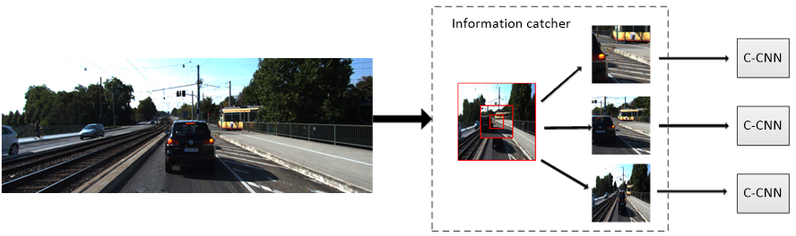
Determine the position of the initial attention point: The position of the initial attention point needs to be given in advance in our method. The first step, the coordinates of the image are converted to [−1,1], and the dot of the image is then set as the center of the image. The coordinates of the initial attention point are obtained by random sampling from the uniform distribution of [−r,r], r ∈ [0,1] under this coordinate system.

Set the parameters: The input of DVAN is the image of KITTI with the size of [376,1242,3] and

Table 1. The structure parameter setting of each sub-module.

Sub-Module	IC	C-CNN	IPM	MOM
		Conv1:$3\times 3\times 3\times 16$
	$S_m=32\times 32$	Conv2:$3\times 3\times 16\times 16$		$O^t\to 256\times 5$
Parameters	N = 3	Conv3:$3\times 3\times 16\times 16$	GRUs:[256] $\times 3$
	$s_f$ = 3	Conv4:$3\times 3\times 16\times 16$		$C^t\to 256\times 3$
	$S_u=64\times 64$	Conv5:$3\times 3\times 16\times 4$
		FC+Relu:$1024\times 256$		$P^{t+1}\to 256\times 2$

shows the specific parameter settings. The structure of all C-CNN is the same, but the parameter settings are slightly different.

3.3. The Setting of Loss Function

The loss function ${\mathrm{L}}_{\mathrm{S}}$ of our network includes three parts, which are the loss part for classification ${\mathrm{L}}_{\mathrm{C}}$, the loss part for attention points ${\mathrm{L}}_{\mathrm{p}}$, and the loss part for location ${\mathrm{L}}_{\mathrm{L}}$. Additionally, we can optimize the entire network structure by minimizing ${\mathrm{L}}_{\mathrm{S}}$.

The loss of classification part (${\mathrm{L}}_{\mathrm{C}}):$ Our method employs the cross entropy loss function to measure the accuracy of the predicted distribution ${\mathrm{C}}^{\mathrm{t}}$ and the real distribution ${\mathrm{C}}^{\mathrm{g}}$ of each category. Additionally, Formula (12) shows the expression of the loss part for classification ${\mathrm{L}}_{\mathrm{C}}$, where N represents the number of categories and ${\mathrm{C}}_{\mathrm{k}}^{\mathrm{g}}$ and ${\mathrm{C}}_{\mathrm{k}}^{\mathrm{t}}$ represent the k-th component of ${\mathrm{C}}^{\mathrm{g}}$ and ${\mathrm{C}}^{\mathrm{t}}$, respectively.

$${\mathrm{L}}_{\mathrm{C}}={\displaystyle \sum }_{\mathrm{k}=1}^{\mathrm{N}}-{\mathrm{C}}_{\mathrm{k}}^{\mathrm{g}}\ln \left({\mathrm{C}}_{\mathrm{k}}^{\mathrm{t}}\right)$$

(12)

The loss of attention point part (${\mathrm{L}}_{\mathrm{p}})$: The role of attention points is to provide C-CNN with feature points for extracting information. The prediction process by constraining attention points with ${\mathrm{L}}_{\mathrm{p}}$ can ensure more accurate local feature extraction. We use the strategy reward mechanism in reinforcement learning [33] to optimize the decision process of attention points, according to the particularity of attention point prediction. Figure 6 shows the optimization process.

In our work, the Agent represents the attention point ${\mathrm{P}}^{\mathrm{t}+1}$ to be predicted. The action of the attention point ${\mathrm{P}}^{\mathrm{t}}$ represents the search of the driver’s interest target or region by the attention point. The Reward is the overlap between the predicted frame and the real frame. The Environment represents the currently processed image. The state represents the accuracy of the search for the driver’s region of interest by the attention point. Additionally, ${\mathrm{R}}^{\mathrm{t}+1}$ and ${\mathrm{S}}^{\mathrm{t}+1}$ are the inputs of Environment to Rward and state, respectively. Moreover, we adopted the L2 loss function to constrain the attention point in the last step, forcing it to approach the center of the target, in order to more accurately simulate the driver’s visual attention mechanism. Accordingly, the loss part ${\mathrm{L}}_{\mathrm{p}}$ of the attention process is expressed as follows, where $\mathsf{\pi }\left(\prime ,″,\prime \right)$ is the distribution of attention points ${\mathrm{P}}^{\mathrm{t}}$, ${\mathrm{b}}^{\mathrm{t}}$ is the expectation of ${\mathrm{R}}^{\mathrm{t}}$, and ${\mathrm{R}}^{\mathrm{t}}$ can be optimized by scoring under the L2 criterion ${\mathrm{O}}_{\mathrm{s}}^{\mathrm{t}}$ to estimate.

$$\begin{gathered} {\mathrm{L}}_{\mathrm{p}}=-{\displaystyle \sum }_{\mathrm{t}=1}^{\mathrm{T}}\ln (\mathsf{\pi }\left({\mathrm{P}}^{\mathrm{t}}|\left({\mathrm{u}}_{\mathrm{p}}^{\mathrm{t}},{\mathsf{\sigma }}^2\right)\right)\left({\mathrm{R}}^{\mathrm{t}}-{\mathrm{b}}^{\mathrm{t}}\right) \\ +\frac{1}{\mathrm{T}}{\displaystyle \sum }_{\mathrm{t}=1}^{\mathrm{T}}{\left({\mathrm{O}}_{\mathrm{s}}^{\mathrm{t}}-{\mathrm{R}}^{\mathrm{t}}\right)}^2+\parallel {\mathrm{u}}^{\mathrm{t}}-\left({\mathrm{O}}_{\mathrm{yx}}^{\mathrm{t}}+\frac{1}{2}{\mathrm{O}}_{\mathrm{hw}}^{\mathrm{t}}\right){\parallel }_2^2 \end{gathered}$$

(13)

The loss of locating part (${\mathrm{L}}_{\mathrm{L}}$): Drivers will pay more attention to dangerous targets or regions ahead of the road during driving. Therefore, we only detect the targets that are most interesting to the driver in the picture in order to simulate this process in a real scenario. The coordinates of the upper left point are ${\mathrm{O}}_{\mathrm{yx}}^{\mathrm{t}}$ and the size is ${\mathrm{O}}_{\mathrm{hw}}^{\mathrm{t}}$. We estimate the predicted amount ${\mathrm{O}}_{\mathrm{yx}}^{\mathrm{P}}$ of the location by means of the maximum contingent estimation. In addition, we also construct a loss function that is related to the predicted border size ${\mathrm{O}}_{\mathrm{hw}}^{\mathrm{P}}$ by predicting the overlap (IOU) of the border and the real border. At the same time, the accuracy of the predicted border is improved by maximizing the IOU. The loss of the positioning portion can be expressed as Equation (14).

$${\mathrm{L}}_{\mathrm{L}}=-\ln \left(\mathrm{P}\left({\mathrm{O}}_{\mathrm{yx}}^{\mathrm{P}}\right)\right)-\ln (\mathrm{IOU}\left({\mathrm{O}}_{\mathrm{hw}}^{\mathrm{P}},{\mathrm{O}}_{\mathrm{hw}}^{\mathrm{t}},{ \mathrm{O}}_{\mathrm{yx}}^{\mathrm{P}},{ \mathrm{O}}_{\mathrm{yx}}^{\mathrm{t}}\right))$$

(14)

Therefore, the loss function in our network is obtained by adding three parts, i.e., ${\mathrm{L}}_{\mathrm{S}}={\mathrm{L}}_{\mathrm{C}}+{\mathrm{L}}_{\mathrm{p}}+{\mathrm{L}}_{\mathrm{L}}$.

3.4. Experimental Results and Analysis

Figure 7 shows the results of this experiment and the change of the loss function during training. The graph (a) is the process variation graph of loss function and the graph (b) shows the final result of the verification of the method on the test set, where the mAP value reaches 79.3%, the overlap (IOU) reaches 58.6%, and the accuracy reaches 96.3%.

In addition, we employ Yolov2 and Yolov3 to train the data set in this paper and perform experimental comparison in order to verify the superiority of our method in real-time detection. The hardware configuration of the experimental environment is NVIDIA GTX1080 video card and 16GB of memory. The programming environment is Tensorflow. We compared the Frames Per Second (FPS) and the accuracy between different networks to show the performance of our method. Figure 8 shows the comparison results. It can be clearly seen from graph (a) that the FPS of our method is slightly lower than that of Yolov2, and it is about the same as that of Yolov3, which is sufficient for meeting the real-time requirements. It can be seen from graph (b) that the three networks have little difference in accuracy, which might be because we only detect three types of targets.

4. Validation

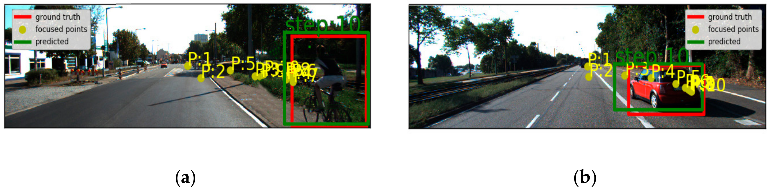
In real traffic scenes, the driver’s attention to important traffic elements as well as his immediate cognition and coping with complex road scenes is one of the most important factors affecting driving safety. In the process of driving, drivers can obtain various information of road traffic through visual search. For the driver’s visual attention mechanism, the driver will not pay the same attention to all targets in the field of vision during driving, but will pay more attention to the targets or regions of most interest. Thus, it is more efficient to directly detect dangerous targets or regions in front of the road, and pay more attention to some relatively important regional targets in the image. We set the number of searches for targets on each picture to 10, that is, the number of points of attention P to 10, so as to better mine context information, in order to verify that our method can simulate the driver’s visual attention mechanism. At the same time, we analyze the sparse traffic scene, the crowded traffic scene, and the intersection traffic scene, respectively, in order to verify that the method can deal with different traffic environments.

Figure 9 shows the traffic scenes with sparse vehicles, which is extremely common in country roads. The traffic scenes in graph (a) and graph (b) are very similar. In these scenes, the vehicles are sparse, but there are targets that may affect the travel in the immediate right front of our vehicles, where graph (a) shows cyclist and graph (b) shows a red vehicle. In this case, the driver should pay more attention to cyclist and the red vehicle in order to prevent traffic accidents. It can be clearly seen from graph (c) and (d) that the targets affecting the forward movement of the vehicle are exactly the opposite of those shown in graph (a) and (b), and are located in the front left of the vehicle. Our method can also accurately locate them. In particular, the car in graph (d) is meeting with a car and another car is moving slowly in the distance, in which case the driver will pay full attention to the silver vehicle with which he meets. According to the above analysis, our method can accurately locate the driver’s most interesting regions in the traffic scenes with sparse vehicles.

Figure 10 shows the traffic scenes with heavy traffic. For the traffic scenes in graph (a) and (b), there are many vehicles in the driver’s field of vision. Not only are there vehicles parked on both sides of the road, but also vehicles in front of them. At this moment, our car is passing through the middle of the road and it is getting closer to the vehicle in front of the left. The driver needs to pay more attention to the vehicle in front of the left in order to prevent collisions. In the traffic scene in graph (c), our car is driving on the highway, and there are many vehicles. Although there are vehicles in front of the own lane, the black vehicle in the adjacent lane is closer to the vehicle and is more prone to collisions. Therefore, the driver will pay more attention to this car. It can be clearly seen from graph (d) that the car meets with a white car on a road with many vehicles. In this scene, the driver will pay full attention to the white car meeting with it. From the above analysis, we know that our method can accurately locate the driver’s most interesting regions in the traffic scenes with heavy traffic.

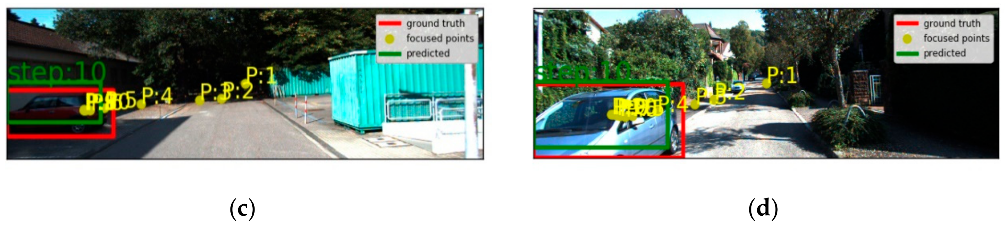
Figure 11 shows the traffic scenes at the intersection. The road conditions at city intersections are very complex, and drivers need to pay more attention to them. Therefore, the effectiveness of our method can be verified to the maximum extent under this scenario. Graph (a) shows the traffic scene, where our car is about to enter the main road from the side road. In this case, the driver pays attention to many regions, but only in the case of graph (a), the driver’s current view is relatively wide and there is no obvious danger information. Therefore, the driver pays more attention to fast moving vehicles in order to avoid potential dangers. In the scene of graph (b), a white vehicle passes in our vertical lane, and the white vehicle is completely exposed to the driver’s field of vision. In this traffic scene, the driver will focus on the white vehicle to prevent traffic accidents.

The scenes in graph (c) and (d) are basically similar, where our cars are waiting for red lights at the intersection. The difference is that there is a red car in front of our car in the graph (c), so the driver will pay more attention to the red car and follow it slowly through the intersection. In graph (d), our car and the white vehicle in the adjacent lane are waiting for the red light together. The driver will pay attention to the white vehicle on the adjacent lane in order to prevent scratches and other accidents at the intersection. According to the above analysis, our method can accurately locate the driver’s most interesting regions in the traffic scenes at the intersection.

5. Conclusions

The current intelligent driving systems do not systematically consider the selective attention mechanism of human drivers, and cannot completely replace the drivers to extract effective road information. This paper proposes a Driver’s Visual Attention Network based on the theory of deep learning and attention model, which is used to simulate the driver’s search and recognition of key road information during driving by predicting the driver’s attention points, to solve this problem. In the experimental part, we first use KITTI dataset for training, and then analyze the three traffic scenes of sparse vehicles, crowded vehicles, and intersections respectively. The experimental results show that the driver’s visual attention mechanism can be simulated in both complex and simple traffic scenes to extract the information of the target or region of the driver’s greatest interest.

References

1. Singh, S. Critical reasons for crashes investigated in the national motor vehicle crash causation survey. In Traffic Safety Facts—Crash Stats; NHTSA: Washington, WA, USA, 2015. [Google Scholar]
2. Shuanfeng, Z.; Wei, G.; Chuanwei, Z. Extraction method of driver’s mental component based on empirical mode decomposition and approximate entropy statistic characteristic in vehicle running state. J. Adv. Transp. 2017, 2017, 9509213. [Google Scholar]
3. Zhao, S. The implementation of driver model based on the attention transfer process. Math. Probl. Eng. 2017, 2017, 15. [Google Scholar] [CrossRef]
4. Zhao, S.; Zhao, Q.; Bai, Y.; Li, S. A traffic flow prediction method based on road crossing vector coding and a bidirectional recursive neural network. Electronics 2019, 8, 1006. [Google Scholar] [CrossRef] [Green Version]
5. Zhouqiu, Z.; Peng, Z.; Shoutao, X.; XingDong, W. Object detection with deep learning: A review. IEEE Trans. Neural Netw. Learn. Syst. 2019, 30, 3212–3232. [Google Scholar]
6. Girshick, R.; Donahue, J.; Darrell, T.; Jitendra, M. Rich feature hierarchies for accurate object detection and semantic segmentation. In Proceedings of the IEEE Conference on Computer Vision and Pattern Recognition, Belfast, UK, 22 October 2014; pp. 580–587. [Google Scholar]
7. Ren, S.; He, K.; Girshick, R.; Jian, S. Faster R-CNN: Towards real-time object detection with region proposal networks. IEEE Trans. Pattern Anal. Mach. Intell. 2017, 39, 1137–1149. [Google Scholar] [CrossRef] [Green Version]
8. Redmon, J.; Divvala, S.; Girshick, R.; Farhadi, A. You only look once: Unified, real-time object detection. In Proceedings of the IEEE Conference on Computer Vision and Pattern Recognition, Las Vegas, NV, USA, 26 June–1 July 2016; pp. 779–788. [Google Scholar]
9. Redmon, J.; Farhadi, A. YOLO 9000: Better, faster, stronger. In Proceedings of the IEEE Conference on Computer Vision and Pattern Recognition, Honolulu, HI, USA, 22–25 July 2017; pp. 6517–6525. [Google Scholar]
10. Ioffe, S.; Szegedy, C. Batch normalization: Accelerating deep network training by reducing internal covariate shift. arXiv 2015, arXiv:1502.03167. [Google Scholar]
11. He, K.; Xiangyu, Z.; Ren, S.; Jian, S. Deep residual learning for image recognition. arXiv 2015, arXiv:1502.03167. [Google Scholar]
12. Yilin, T.; Dollár, P.; Girshick, R.; He, K.; Hariharan, B.; Belongie, S. Feature pyramid networks for object detection. arXiv 2016, arXiv:1612.03144. [Google Scholar]
13. Redmon, J.; Farhadi, A. Yolov3: An incremental improvement. arXiv 2018, arXiv:1804.02767. [Google Scholar]
14. Putra, M.H.; Yussof, Z.M.; Lim, K.C.; Salim, S.I. Convolutional neural network for person and car detection using YOLO framework. J. Telecommun. Electron. Comput. Eng. 2018, 10, 67–71. [Google Scholar]
15. Zhongbao, Z.; Hongyuan, W.; Ji, Z.; Yang, W. A vehicle real-time detection algorithm based on YOLOv2 framework. In Real-Time Image and Video Processing 2018; International Society for Optics and Photonics: Bellingham, WA, USA, 2018; Volume 10670. [Google Scholar]
16. Liu, W.; Anguelov, D.; Erhan, D.; Szegedy, C.; Reed, S.; Fu, C.; Berg, A.C. SSD: Single shot multibox detector. In Proceedings of the European Conference on Computer Vision, Amsterdam, The Netherlands, 8–16 October 2016; pp. 21–37. [Google Scholar]
17. Kim, H.; Lee, Y.; Yim, B.; Park, E. On-road object detection using deep neural network. In Proceedings of the IEEE International Conference on Consumer Electronics-Asia (ICCE-Asia), Seoul, Korea, 26–28 October 2016; Volume 201, pp. 1–4. [Google Scholar]
18. Alletto, S.; Palazzi, A.; Solera, F.; Calderara, S.; Cucchuara, R. Dr (eye) ve: A dataset for attention-based tasks with applications to autonomous and assisted driving. In Proceedings of the IEEE Conference on Computer Vision and Pattern Recognition Workshops, Las Vegas, NV, USA, 26 June–1 July 2016; pp. 54–60. [Google Scholar]
19. Alletto, S.; Palazzi, A.; Solera, F.; Calderara, S.; Cucchuara, R. Learning where to attend like a human driver. In Proceedings of the IEEE Intelligent Vehicles Symposium, Redondo Beach, CA, USA, 11–14 June 2017; pp. 920–925. [Google Scholar]
20. Palazzi, A.; Abati, D.; Calderara, S. Predicting the driver’s focus of attention: The DR (eye) VE project. IEEE Intell. Veh. Symp. 2019, 41, 1720–1733. [Google Scholar] [CrossRef] [Green Version]
21. Tawari, A.; Kang, B. A computational framework for driver’s visual attention using a fully convolutional architecture. In Proceedings of the IEEE Intelligent Vehicles Symposium, Redondo Beach, CA, USA, 11–14 June 2018; pp. 887–894. [Google Scholar]
22. Jaderberg, M.; Karen, S.; Zisserman, A. Spatial transformer networks. arXiv 2015, arXiv:1506.02025. [Google Scholar]
23. Jie, H.; Shen, L.; Gang, S. Squeeze-and-excitation networks. arXiv 2017, arXiv:1709.01507. [Google Scholar]
24. Bo, Z.; Xiao, W.; Jiashi, F.; Qiang, P.; Shuicheng, Y. View all authors diversified visual attention networks for fine-grained object classification. IEEE Trans. Multimed. 2017, 19, 1245–1256. [Google Scholar]
25. Oliva, A.; Torralba, A. The role of context in object recognition. Trends Cogn. Sci. 2007, 11, 520–527. [Google Scholar] [CrossRef]
26. Mnih, V.; Heess, N.; Graves, A. Recurrent models of visual attention. arXiv 2014, arXiv:1406.6247. [Google Scholar]
27. Torralba, A.; Oliva, A.; Castelhano, M.S.; Henderson, J.M. Contextual guidance of eye movements and attention in real-world scenes: The role of global features in object search. Psychol. Rev. 2006, 113, 766–786. [Google Scholar] [CrossRef] [Green Version]
28. Chung, J.; Gulcehre, C.; Cho, K.; Bengio, Y. Empirical evaluation of gated recurrent neural networks on sequence modeling. arXiv 2014, arXiv:1412.3555. [Google Scholar]
29. Hocheiter, S.; Schmidhuber, J. Long short-termmemory. Neural Comput. 1997, 9, 1735–1780. [Google Scholar] [CrossRef]
30. Theeuwes, J. Top-down and bottom-up control of visualselection. Acta Psychol. 2010, 135, 77–99. [Google Scholar] [CrossRef]
31. Hayhoe, M.; Ballard, D. Eye movements in natural behavior. Trends Cogn. Sci. 2005, 9, 188–194. [Google Scholar] [CrossRef]
32. Geiger, A.; Lenz, P.; Urtasun, R. Are we ready for autonomous driving? The KITTI vision benchmark suite. In Proceedings of the IEEE Conference on Computer Vision and Pattern Recognition, Providence, RI, USA, 16–21 June 2012. [Google Scholar]
33. Williams, R.J. Simple statistical gradient-following algorithms for connectionist reinforcement learning. Mach. Learn. 1992, 8, 229–256. [Google Scholar] [CrossRef] [Green Version]
Figure 1. The overall structure of driver’s visual attention network (DVAN).
Applsci 10 01083 g001
Figure 2. The effect diagram of Information Capture (IC).
Applsci 10 01083 g002
Figure 3. The schematic diagram of Cross Convolutional Neural Network (C-CNN).
Applsci 10 01083 g003
Figure 4. The structure diagram of Gate Recurrent Unit (GRU).
Applsci 10 01083 g004
Figure 5. The part of data set display diagram.
Applsci 10 01083 g005
Figure 6. The training process of attention point.
Applsci 10 01083 g006
Figure 7. The training results of our experiment. (a) The training process of loss; (b) the values of the three indicators.
Applsci 10 01083 g007
Figure 8. The comparison between our method and other networks. (a) The comparison of Frames Per Second (FPS); and, (b) the comparison of accuracy.
Applsci 10 01083 g008
Figure 9. The four situations in traffic scenes with sparse vehicles. (ad) shows four different situation, respectively.
Applsci 10 01083 g009aApplsci 10 01083 g009b
Figure 10. The four situations in traffic scenes with heavy traffic. (ad) shows four different situation, respectively.
Applsci 10 01083 g010
Figure 11. The four situations in the intersection traffic scene. (ad) shows four different situation, respectively.
Applsci 10 01083 g011