Article

Theoretical Analysis of Fractional Viscoelastic Flow in Circular Pipes: Parametric Study

1
Department of Mechanical and Industrial Engineering, University of Illinois at Chicago, Chicago, IL 60607, USA
2
Computational Science Division and Leadership Computing Facility, Argonne National Laboratory, Lemont, IL 60439, USA
*
Author to whom correspondence should be addressed.
Appl. Sci. 2020, 10(24), 9080; https://doi.org/10.3390/app10249080
Submission received: 29 October 2020 / Revised: 7 December 2020 / Accepted: 14 December 2020 / Published: 18 December 2020

Abstract

:
Pipe flow is one of the most commonly used models to describe fluid dynamics. The concept of fractional derivative has been recently found very useful and much more accurate in predicting dynamics of viscoelastic fluids compared with classic models. In this paper, we capitalize on our previous study and consider space-time dynamics of flow velocity and stress for fractional Maxwell, Zener, and Burgers models. We demonstrate that the behavior of these quantities becomes much more complex (compared to integer-order classical models) when adjusting fractional order and elastic parameters. We investigate mutual influence of fractional orders and consider their limiting value combinations. Finally, we show that the models developed can be reduced to classical ones when appropriate fractional orders are set.

1. Introduction

Fractional calculus in general and fractional derivative in particular has been gathering an increasing researchers interest recently. This mathematical tool provides the means for significant improvement of predictive power for numerous practical applications as summarized in a recent literature [1,2,3,4,5,6,7,8,9,10,11,12,13,14,15,16,17,18]. Heat conduction [5,18], anomalous diffusion [4,7], and viscoelastic properties of fluids and solids [3,9,10,13] are just a few examples of fundamental phenomena where fractional calculus finds immediate practical applications and provides promising results. While fractional models in general demonstrate better fit of experimental data compared to their classical counterparts, those involving variable-order fractional operators (VO-FC) are the handy tools for the cutting-edge research. VO-FC not only provides an effective tool to alter the system properties described by the fractional orders but also allows accounting for fractional orders variations with time, coordinate, and internal system-specific parameters.
One of the fields where fractional calculus has already proven its efficiency is the prediction of dynamics of viscoelastic flows in various constrained geometries, with circular pipe being one of the most popular ones. With theoretical foundations laid in [19], researchers considered numerous specific problems. The models studied here were addressed by Yin in [20] (Maxwell), by Shah in [21] (Burgers) to name a few. Fractional viscoelastic models, including Maxwell and Zener ones, were considered in close detail in series of works by Schiessel, Friedrich, and others [22,23]. Those authors provided in-depth physical analysis of mathematical concepts introduced via fractional calculus formalism, suggested, developed, and explained various ladder models. This brief literature overview is intended to mention the most recent achievements in a field of FC and to point out studies that specifically targeted fractional models studied here. A more detailed consideration that includes historic retrospective can be found in our previous study [1].
In this paper, we capitalize on the approaches developed in [1] to examine the behavior of fractional viscoelastic Maxwell, Zener, and Burgers models in application to pipe flow. We present an in-depth parametric analysis of these models and outline various operating regimes for each of them. Different from [1], here we consider 3D profiles of flow velocity and stress. It allows for the exploration of flow dynamics in spatial and frequency domains simultaneously and catches the specifics that cannot be easily visible in 2D projections. We consider various combinations of fractional orders, investigate their mutual influence, and establish an approach for viscoelastic flow optimization. The paper is organized as follows. We first provide domain definition. The governing equations for fluid flow and constitutive equations for the model considered are given in Section 2.1 and Section 2.2, respectively. The main results of this study appear in Section 3. In particular, Section 3.1 describes the general approach for seeking the solution. Section 3.2, Section 3.3, Section 3.4, Section 3.5, Section 3.6 and Section 3.7 present and discuss space-frequency dynamics of velocity and stress profiles. In particular, Section 3.2 presents velocity for fractional Maxwell model. Stress profiles for fractional Maxwell model are considered in Section 3.3. Zener model behavior is studied in Section 3.4 and Section 3.5 (velocity and stress, respectively). Section 3.6 and Section 3.7 are devoted to fractional Burgers model. The results of this study are summed up in Section 4. Hereafter we use the following notions. Under “classic” we understand either model or profile corresponding to integer values of fractional orders. “Fractional order” and “fractional parameter” is essentially the same. We also use “frequency domain” to refer to nondimensional frequency.

2. Problem Formulation

Here we provide brief problem formulation and key governing equations. All the details as well as derivations and overview of mathematical apparatus involved can be found in our previous study [1].
Let us introduce cylindrical coordinate system ( r , θ , z ) and consider laminar flow of incompressible viscoelastic fluid along z axis of infinitely long pipe of radius R with circular cross-section. The corresponding schematic is shown in Figure 1.

2.1. Flow Dynamics

cyanThe flow dynamics is governed by continuity and momentum equations with no-slip boundary condition at the wall applied. Due to flow and geometry specifics, only z-component of momentum equation remains and reads as:
ρ u z t = p z + 1 r ( r σ r z ) r
Here ρ , u z , p , σ r z stand for fluid mass density, z-component of flow velocity, pressure, and r z -component of stress.

2.2. Constitutive Equations

First, we consider fractional Maxwell model (Figure 2a). Its constitutive equation reads as:
σ ( t ) + τ a α β D t α β σ ( t ) = E τ a α D t α ε ( t ) , 0 α 1 , 0 β 1 , α β
Here α and β are the fractional orders, τ , E are given by:
τ = E 1 τ 1 α E 2 τ 2 β 1 α β , E = E 1 τ 1 τ α , E = E 2 τ 2 τ β ,
where E 1 , τ 1 , E 2 , τ 2 stand for the Young’s moduli, relaxation times of elements “1” and “2”, respectively. The ranges imposed for α and β have both physical and mathematical meaning. Physically, changing α and β from 0 to 1 allows balancing between viscous and elastic properties of fluid. Mathematically, all fractional orders should be non-negative, in order to ensure that we deal with fractional derivatives, not fractional integrals. An additional relation bounds α and β , so that the entire range for β can only be considered provided α = 1 . The limiting integer values of fractional orders deserve special attention, as they allow restoring various classical cases. In particular, α = 1 and β = 0 correspond to the classical Maxwell fluid:
σ + τ σ ˙ = E τ ε ˙ ,
while α = 1 and β = 1 results in a constitutive equation for the Newtonian fluid:
σ = E τ 2 ε ˙
Here we omitted time dependence of stresses and strains for brevity and introduced dot as a time derivative operator. A closer look at the definition of τ reveals that the case α = β is somewhat special. Indeed, it corresponds to a critical gel. It means that τ blows up when α = β . However, it happens when the base (expression in brackets) is greater than unity. If the opposite is true, then τ is bounded. However, the detailed analysis of all the specifics it brings is beyond the scope of this study.
Next, we consider fractional Zener model shown in Figure 2b. In this case constitutive equation is:
σ ( t ) + τ a α β D t α β σ ( t ) = E τ a α D t α ε ( t ) + E 0 τ a γ D t γ ε ( t ) + E 0 τ a γ + α β D t γ + α β ε ( t ) , 0 α 1 , 0 β 1 , 0 γ 1 , α β 0 , γ + α β 0
Here γ is the fractional order of element “3” and E 0 is defined as:
E 0 = E 3 τ 3 τ γ ,
where E 3 , τ 3 stand for Young’s modulus and relaxation time of element “3” and all other notations are the same as above. At a glance, here we end up with two additional relations for the fractional orders α , β , and γ : α β 0 and γ + α β 0 . A closer look to this inequalities reveals that if α β 0 is held, the second one is satisfied automatically. That is, of course, only true for non-negative values of the fractional orders. To get classical Zener fluid, one should assume α = 1 , β = 0 , and γ = 0 . Then the constitutive equation reduces to:
σ + τ σ ˙ = E 0 ε + ( E + E 0 ) τ ε ˙
Next, assuming α = 1 , β = 1 , and γ = 1 , one will end up with Newtonian fluid and constitutive equation of the form:
σ = E + 2 E 0 2 τ ε ˙
Finally, for fractional Burgers model, (Figure 2c) we have:
σ ( t ) + E E 0 τ a α γ D t α γ σ ( t ) + E E 0 τ a α δ D t α δ σ ( t ) + E E 0 τ a β γ D t β γ σ ( t ) + E E 0 τ a β δ D t β δ σ ( t ) = = E τ a α D t α ε ( t ) + E τ a β D t β ε ( t ) , 0 α 1 , 1 β 2 , 0 γ 1 , 0 δ 1 , α γ 0 , β γ 0 , α δ 0 , β δ 0
Here δ is the fractional order of element “4”, (7) is still valid and additionally:
E 0 = E 4 τ 4 τ δ ,
where E 4 , τ 4 stand for Young’s modulus and relaxation time of element “4” and all other notations being the same as above. Here we impose four additional conditions for fractional orders α , β , γ and δ . Different from previous models, the range of β has changed as the classical Burgers model should include second derivatives of stresses and strains with respect to time. Moreover, there are no relations for fractional orders α and β . At the same time, the whole range of values for fractional orders γ and δ can only be considered if α = 1 . To get classical Burgers model, one should set α = 1 , β = 2 , γ = 0 and δ = 0 . Then the constitutive equation reads as:
σ + 2 E E 0 τ ( σ ˙ + τ σ ¨ ) = E τ ( ε ˙ + τ ε ¨ ) ,
where two dots stand for the second derivative with respect to time. Newtonian fluid can be obtained by setting α = β = γ = δ = 1 . Corresponding constitutive equation reads as:
σ = 2 E E 0 E 0 + 4 E τ ε ˙

3. Results and Discussion

3.1. General Solution

Here we follow the approach proposed earlier by Yin [20] for Maxwell model and then generalize it for all other models. Introduce pressure gradient of the form:
p z = P 0 e i ω t
For all models considered in this study, nondimensional velocity and stress profiles are given by:
u ˜ = u z u 0 = 1 J 0 ( ω ¯ a ˜ ϕ ) J 0 ( ω ¯ a ˜ ) , σ ˜ = σ r z σ 0 = J 1 ( ω ¯ a ˜ ϕ ) ω ¯ a ˜ J 0 ( ω ¯ a ˜ ) ,
where we used the following quantities:
r ˜ = r ν τ , a ˜ = R ν τ , ω ˜ = ω τ , ϕ = r ˜ a ˜ , u 0 = 1 4 ρ ω p z , r 2 ξ 2 = ω ¯ r ˜ 2 ,
and ν , ω stand for kinematic viscosity and angular frequency, σ 0 = p z R , and J l ( · ) is the Bessel function of first kind of order l. For all the models considered, we set a ˜ = 0.1 . Table 1 provides expressions for parameter ξ 2 and ranges of fractional orders for all three models. The details of velocity and stress profiles derivation can be found in [1].

3.2. Velocity Profiles for Fractional Maxwell Model

For fractional Maxwell model parameters that can vary are fractional orders α and β . We examine dynamics of normalized velocity along pipe diameter with respect to nondimensional frequency, ω ˜ . Both fractional orders α and β are varied considering α β . Let us first fix β = 0.2 and vary α : α = 0.2 , …, 1 (See Supplementary Materials animation muz1 https://youtu.be/wNkKfdEOS4Q). Alternatively, α = 1 and β is varied as: β = 0.2 , …, 1 (animation muz2 https://youtu.be/2dWZ6KNwL5I). These two velocity profiles have both similarities and distinct differences. Consider similarities first. Oscillatory behavior of the velocity profile is observed with respect to both spatial and frequency coordinates while for the latter these oscillations are also damped. Moreover, up to a certain nondimensional frequency, velocity increases rapidly until forming a nearly parabolic profile. Additionally, with α and β increasing, resonant peaks of velocity profile shift to higher values of non-dimensional frequency. Upon passing this profile, oscillations emerge along the pipe diameter. The dynamics of initial parabolic profile, however, differ when changing α and β . In particular, when β is fixed and α increases, peak amplitudes in initial parabolic profile oscillate. In contrast to it, when we fix α and vary β , initial parabolic profile peak amplitude gradually decreases with increasing β . What is even more noticeable, for α = 1 and β = 0.2 , …, 1, the velocity profile reduces to parabolic for the entire range of nondimensional frequency as β increases. This result is not surprising as for α = 1 and β = 1 we end up with a Newtonian fluid.

3.3. Stress Profiles for Fractional Maxwell Model

Now let us have a look at stress profiles (animations msf1 https://youtu.be/3YnhhJUy1Wg and msf2 https://youtu.be/wTi8FdTpyok). Here again we either fix β = 0.2 and vary α : α = 0.2 , …, 1 (animation msf1 ) or fix α = 1 and vary β : β = 0.2 , …, 1 (animation msf2 ), while satisfying α β . Let us start from the similarities. The profiles are symmetrical with respect to pipe centerline. For both cases, stress exhibits aperiodic oscillations in a frequency domain and increases monotonically (nonlinear) from the pipe center up to the wall. Here come the differences. When β is fixed, stress peak amplitudes oscillate with increasing α in frequency domain with resonant peak shifting to higher values. More specifically, peak amplitude initially decay up to α 0.5 . For α > 0.5 trend reverses. Interestingly, the rate of amplitude change is higher for α < 0.5 . The situation changes dramatically when α = 1 , β = 0.2 , …, 1. While the initial behavior is very similar to the first case, the stress becomes independent of frequency and increases linearly from the pipe center up to the wall as β approaches unity (Newtonian fluid).

3.4. Velocity Profiles for Fractional Zener Model

Fractional Zener model is described by four parameters, namely three fractional orders α , β , γ and elastic parameter ψ ( ψ = E 0 / E ). Let us first set ψ = 1 and examine contributions made by fractional orders α , β , γ . In the first pair of animations (zuz1 https://youtu.be/T8LLEwgiC4k and zuz2 https://youtu.be/dXQCrXTNLbQ) we investigate the influence of fractional order α ( α = 0.2 , …, 1) for two limiting cases of β and γ ( β = γ = 0.2 and β = γ = 1 , respectively). In both cases we observe parabolic profiles along the pipe diameter with the amplitude increasing when so does nondimensional frequency. However, in case of lower limits for fractional orders β and γ , the parabolic profile is followed by complex oscillatory pattern. Moreover, peak values of initial parabolic profile also oscillate. The situation is strikingly different if we consider the upper limit for fractional orders β and γ ( β = γ = 1 ). Here parabolic profile occupies the entire range of nondimensional frequency considered. Moreover, it is independent from fractional order α .
Let us now have a look at the impact of the fractional order β . More specifically, we fix fractional orders α = 1 , γ = 0.2 (animation zuz3 https://youtu.be/bjLWJxFWy8I) and α = 1 , γ = 1 (animation zuz4 https://youtu.be/9VaIO3HkW8Y), while varying β : β = 0.2 , …, 1. Initial velocity profiles look somewhat similar to the previous case. That is, for lower limit value of γ profile is initially parabolic and switches to oscillatory in both space- and frequency domains. For the upper limit of γ , increasing parabolic profile along pipe diameter occupies entire frequency domain. However, it all changes when β start increasing. In particular, velocity profile gradually becomes parabolic along pipe diameter for the entire frequency range thus delivering a case of Newtonian fluid (animation zuz3 https://youtu.be/bjLWJxFWy8I). For the upper limit value of γ (animation zuz4 https://youtu.be/9VaIO3HkW8Y), the amplitudes of parabolic profile gradually decrease (up to roughly 60% from the maximum value) with increasing β .
Next, we investigate the effect of varying fractional order γ . More specifically, we fix α = 1 for both lower limit of β ( β = 0.2 , animation zuz5 https://youtu.be/j8AGHtMGXV8) and upper limit of β ( β = 1 , animation zuz6 https://youtu.be/-wJNeA8hTXY), while varying γ : γ = 0.2 , …, 1. While the plots exhibit some similarities with the case of varying fractional order β , their dynamics is different. In particular, the rate of amplitudes decay for both parabolic and oscillating components is much higher. The same can be said when the profile turns to a parabolic for the entire frequency domain. As for the upper limit value of β , the amplitudes of parabolic profile also decay relatively faster (up to roughly 35% from the maximum value).
Finally, we consider the impact of elastic parameter ψ . More specifically, we fix α = 0.5 and β = 0.2 for both lower (animation zuz7 https://youtu.be/GExLFiUC8Hk) and upper (animation zuz8 https://youtu.be/YbKXMIgcwSY) limits of fractional order γ ( γ = 0.2 and γ = 1 , respectively). At the same time, we vary ψ : ψ = 0.01 100 . For the lower limit of γ , the peak amplitudes of the velocity profile increase until switching happens ( ψ 20 ) from parabolic+oscillatory behavior to purely parabolic. Upon reaching parabolic profile, its amplitudes start decaying while further increasing ψ . The rate of decay, however, decreases with increasing ψ (especially for ψ > 30 ). Different from all other cases with upper limit values of fractional order set, here for γ = 1 we observe a combination of parabolic and oscillatory profiles for lower values of ψ . It changes abruptly to a parabolic one ( ψ 0.1 ) and almost vanish for ψ > 5 . This more complex structure can, however, be attributed to the fact that we set α not at the upper limit value ( α = 1 ) but at α = 0.5 .
Generally speaking, the influence of fractional orders and elastic parameter on a velocity profile is quite different. The strongest effect is achieved when varying elastic parameter ψ . Among fractional orders, the most powerful contribution in a profile dynamics is made by the fractional order γ , while influence of α is the weakest one. This trend is especially visible for the upper limit values of the fractional orders.

3.5. Stress Profiles for Fractional Zener Model

We further consider the dynamics of stress profiles for fractional Zener model. We first fix ψ = 1 and examine the influence of fractional parameters only. We consider the contribution made by the different parameters in the same order as for velocity profiles, i.e., varying α , β , γ and ψ . Let us start from the fractional order α . Corresponding plots are shown in animations zsf1 https://youtu.be/SOV4_XRiL1s and zsf2 https://youtu.be/ajgZpM0JQS8. For the first one we set β = 0.2 , γ = 0.2 and vary α : α = 0.2 , …, 1. As previously, profile is symmetric with respect to the pipe centerline. Moreover, it exhibits abruptly decaying aperiodic oscillations in a frequency domain. As α increases, peak amplitudes of the stress initially reduce, followed by increase for α > 0.5 . Different from fractional Maxwell model (see animation msf1 https://youtu.be/3YnhhJUy1Wg), the rate of peak amplitude change appears to be almost the same for α < 0.5 and α > 0.5 . The stress profile for upper limit values of β and γ is shown in animation zsf2 https://youtu.be/ajgZpM0JQS8. It reveals that the stress is independent from the fractional order α and remains almost the same for the entire frequency domain.
Next, we examine the influence of fractional order β . More specifically, α is fixed ( α = 1 ) with β varying ( β = 0.2 , …, 1) and limiting values of γ . Stress dynamics for γ = 0.2 is given in animation zsf3 https://youtu.be/jSkii6WKFlg. Different from the case with varying α , here we observe switching from oscillatory to constant behavior in a frequency domain as β increases. Stress profile for upper limit of γ ( γ = 1 ) is shown in animation zsf4 https://youtu.be/zpyOc_J-Xnc. It turns out to be very slightly increasing at the pipe walls with increasing β in a frequency domain, while linearly increasing from the pipe center up to its walls.
Let us now vary fractional order γ . We set α = 1 ; β = 0.2 (animation zsf5 https://youtu.be/M72Hy5s1D_U) or β = 1 (animation zsf6 https://youtu.be/A-yh4HRlXz4) and vary γ : γ = 0.2 , …, 1. Here again we observe a switch from oscillatory to V-shape profile with increasing γ ( β = 0.2 ). When β = 1 , V-shape profile is present for the entire range of γ . It slightly decays at the pipe walls. However, this decay vanishes with increasing γ to to being completely independent from ω ˜ .
Finally, we looked at the difference made by varying elastic parameter ψ . We fixed α = 0.5 , β = 0.2 , vary ψ ( ψ = 0.01 100 ). The lower limit case ( γ = 0.2 ) is given in animation zsf7 https://youtu.be/qlLd7LQ6mtw. Switching between oscillatory and V-shape profiles is observed. However, its dynamics is different from the cases of varying fractional orders. More specifically, the peak stress values first increase with increasing ψ . This trend is observed until switching to V-shape profile, when stress amplitudes start gradually decrease. Next, we set γ = 1 (animation zsf8 https://youtu.be/WqIpXuk0tG8). Here too, a drastic difference from all the cases with varying fractional orders is observed. That is, complex symmetric oscillatory profile is present for the lowest values of ψ . As ψ starts increasing, stress amplitudes drop abruptly and switching to a V-shape profile occurs. Upon reaching this point, stress amplitude at the pipe walls starts growing.

3.6. Velocity Profiles for Fractional Burgers Model

Finally, let us examine the most complex model presented in this study, fractional Burgers model. Here five parameters should be considered, namely four fractional orders α , β , γ , δ and elastic parameter ψ . Here we follow the pattern used above to maintain consistency. In particular, we first fix elastic parameter value and study the influence of fractional parameters on model dynamics and then include varying elastic parameter in consideration. To demonstrate the model to be universal, we picked a different value of elastic parameter, ψ = 10 , when varying fractional orders α , β , γ and δ . It is worth remembering that for fractional Burgers model the range of fractional order β is different ( 1 β 2 ) from those for fractional Maxwell and Zener model ( 0 β 1 ).
As previously, let us start from a varying fractional order α ( α = 0.2 , …, 1). We fix β = 1.2 and consider lower ( γ = 0.2 , δ = 0.2 ) and upper ( γ = 1 , δ = 1 ) limits of the fractional orders γ and δ . Corresponding plots are shown in animations buz1 https://youtu.be/tLqceVl3ywk and buz2 https://youtu.be/JlIdYSZ-hbk. For lower limit values of fractional orders γ and δ , velocity profile appears to be independent from the fractional order α . Moreover, profile itself looks different from those fractional Maxwell and Zener models (for varying α ). In particular, as nondimensional frequency increases, the velocity profile changes from parabolic to a resonant with plateaus. This difference, however, can be attributed to the fact that we picked a different value of elastic parameter ψ . When upper limit values of γ and δ are considered, velocity profile changes to parabolic with gradually increasing amplitude for the entire frequency domain. As α increases, no changes in profile shape are observed until α 0.6 . Starting from it, peak profile value starts decreasing and reduces by approximately 40%.
Next, we fix α = 1 and consider the impact of fractional order β . Velocity profile for lower limit of the remaining fractional orders ( γ = 0.2 , δ = 0.2 ) is given in animation buz3 https://youtu.be/TUZE3HmaUg8. While the initial profile looks similar to the previous case, its dynamics with β differs. More specifically, profile consists of parabolic and resonant profiles. As β increases, peak value of parabolic profile slowly increases. Upon reaching β 1.8 it remains almost unchanged. In contrast to it, as shown in animation buz4 https://youtu.be/Cp6h-9S-7hA, for γ = δ = 1 , there is only parabolic profile present for the entire frequency domain. Its peak amplitudes decrease gradually with increasing β dropping by approximately 70% from their maximum values. Moreover, as β surpasses a certain value ( β 1.7 ), profile remains almost unchanged up to upper limit ( β = 2 ).
Now let us have a look at the influence made by varying fractional order γ . More specifically, we fix α = 1 , consider lower ( β = 1 , δ = 0.2 ) and upper ( β = 2 , δ = 1 ) limits for fractional orders β and δ . Finally, we vary γ in a range: γ = 0.2 , …, 1. For the lower limit (animation buz5 https://youtu.be/X2DWL3tJDV8) we start with a combination of parabolic and resonant profiles. As γ increases, peak value amplitudes for both components gradually decrease. Simultaneously, the profile degenerates to a parabolic for the entire frequency domain. These trends are observed up to γ 0.6 . Upon passing this value, profile remains parabolic. Its peak amplitude starts slowly increasing up to the limit value ( γ = 1 ). When it comes to upper limit ((animation buz6 https://youtu.be/hs7pUv2nybo)), dynamic parabolic profile is observed for the entire frequency domain. It, however, has some specifics that distinguishes it from previous cases. That is, for lower values of γ , peak values of parabolic profiles approach resonance at a certain ω ˜ , then starts decaying, and finally reaches nearly constant value. The situation, however, changes when γ starts increasing. Peak values of parabolic profile start reducing until peak itself disappears. Then for the entire frequency domain parabolic profile is observed with amplitudes gradually increasing with ω ˜ .
The last, but the least fractional order to vary is δ . Other fractional orders are as follows: α = 1 ; β = 1 , γ = 0.2 (lower limit) and β = 2 , γ = 1 (upper limit). Finally, δ = 0.2 , …, 1. Lower limit case is given in animation buz7 https://youtu.be/wmkBTIXXI0I. Similar to animation buz5 https://youtu.be/X2DWL3tJDV8, where we varied γ , a combination of parabolic and resonant profiles is observed. With δ increasing it degenerates to a parabolic profile for the entire frequency range with a resonance at a certain ω ˜ . For the upper limit (animation buz8 https://youtu.be/0UQ6tFeV3yc) the profile is overall similar to animation buz6 https://youtu.be/hs7pUv2nybo, where varying γ was considered.
Finally, we consider the impact made by a varying elastic parameter ψ . Here ψ changes in a range ψ = 0.1 , …, 100. We start from α = 1 , β = 1 , γ = 0.2 and δ = 0.2 (animation buz9 https://youtu.be/t_BV2foEg5w). The profile dynamics appears to be the most complex considered so far. For the lowest values of ψ we have a combination of parabolic profile, inclined decaying oscillations that are symmetric with respect to pipe centerline. The latter enclose a plateau. As ψ increases, this complex combination transforms to parabolic+oscillatory profile observed for fractional Maxwell and Zener models. Next, it turns to a combination of parabolic and resonant profiles. With further increase in ψ , parabolic profile with resonance at certain ω ˜ emerges. Finally, it becomes a simple parabolic profile with the amplitude increasing with ω ˜ . The next set of fractional parameters considered is: α = 1 , β = 2 , γ = 0.2 , and δ = 0.2 (animation buz10 https://youtu.be/Fyel0IDrbtU). The variety of the profiles remains the same. However, in this case switching between them occurs slower compared to the previous one. Moreover, relative peak amplitudes turn out to be higher. Two final profiles correspond to parameter sets: α = 1 , β = 1 , γ = 1 , δ = 1 and α = 1 , β = 2 , γ = 1 , δ = 1 (animations buz11 https://youtu.be/MboUM5_YEM0 and buz12 https://youtu.be/U7uPEOWOc5s, respectively). This pair appears to be a way more simpler compared its immediate predecessors. More specifically, for both cases plots represent a combination of parabolic and M-shape profiles. Both reduce to simple parabolic profiles as ψ increases, with amplitudes increasing when so does ω ˜ . In contrast to animation buz10 https://youtu.be/Fyel0IDrbtU, in animation buz12 https://youtu.be/U7uPEOWOc5s relative peak amplitudes decay faster for the upper limit of β ( β = 2 ). Relative simplicity of these two profiles can be attributed to the fact that all fractional orders as well as their differences are set to integers.

3.7. Stress Profiles for Fractional Burgers Model

Finally, we will have a look at the dynamics of stresses for fractional Burgers model. In picking the values for parameters affecting system behavior, we pursue the logic developed for the velocity profiles. In particular, we first fix the value of the elastic parameter at ψ = 10 , set limiting values for three out of four fractional parameters and vary the fourth one. Then vary ψ for various limiting values of fractional orders. Once again, let us start from varying fractional order α ( α = 0.2 , …, 1). Simultaneously, we set β = 1.2 , γ = 0.2 , δ = 0.2 for lower limit (animation bsf1 https://youtu.be/Pa3jHar4Ld8) and β = 1.2 , γ = 1 , δ = 1 for the upper limit (animation bsf2 https://youtu.be/mTf29Vn1TSQ). When compared to animations zsf1 https://youtu.be/SOV4_XRiL1s and zsf2 https://youtu.be/ajgZpM0JQS8 for fractional Zener model, both similarities and differences can be outlined. For upper limit values, stresses are independent from α and do not change in frequency domain. For lower limit, plots have similar structure and are independent from α . At the same time, for Zener model major peak is sharper and higher, while for Burgers it has lower peak amplitude and is way more dispersive.
Next, we fix α = 1 and consider the impact of fractional order β . Velocity profile for lower limit of the remaining fractional orders ( γ = 0.2 , δ = 0.2 ) is given in animation bsf3 https://youtu.be/UdAFrW3Ut-8. It differs dramatically from a similar plot for fractional Zener model (animation zsf3 https://youtu.be/jSkii6WKFlg). In particular, while aperiodic oscillations are also observed in both frequency and space domains, no switching to V-shape profile occurs. Instead, amplitude of major peak slowly increases with increasing β . As for the upper limit ( γ = 1 , δ = 1 ), static V-shape profile is observed.
Now let us have a look on the influence made by varying fractional order γ . More specifically, we fix α = 1 , consider lower ( β = 1 , δ = 0.2 ) and upper ( β = 2 , δ = 1 ) limits of fractional orders β and δ . Finally, we vary γ in a range: γ = 0.2 , …, 1. For lower limit, plot is shown in animation bsf5 https://youtu.be/eRX9wVxeW_Y. It exhibits aperiodic oscillations in both space- and frequency domains. As γ increases, the value of the major peak increases too. Moreover, the peak itself shifts to higher values of ω ˜ . When compared to appropriate Zener model (animation zsf5 https://youtu.be/M72Hy5s1D_U), a striking difference can been seen. More specifically, for Zener model, increasing γ results in switching profile from oscillating to V-shape. For the upper limit, plot is given in animation bsf6 https://youtu.be/owVOe5Nvc9Q. As γ increases, it demonstrates switching between oscillatory and V-shape profiles. When compared to appropriate Zener model (animation zsf6 https://youtu.be/A-yh4HRlXz4), the major difference is that for the latter only V-shape profile is present.
Next in line, we consider varying fractional order δ ( δ = 0.2 1 ). Corresponding plots for lower limit ( α = 1 , β = 1 , γ = 0.2 ) and upper limit ( α = 1 , β = 2 , γ = 1 ) are shown in animations bsf7 https://youtu.be/8H_w4KVlAp8 and bsf8 https://youtu.be/Djga0UAMybI, respectively. We start with the lower limit case. Here we observe aperiodic oscillatory behavior of the stress profile. As δ increases up to δ 0.5 , amplitudes of the major peaks decrease. Upon passing this point, trend reverses and peak amplitudes start increasing up to the upper limit of δ ( δ = 1 ). For the upper limit case switching between aperiodic oscillatory and V-shape profiles occurs as δ increases. Interestingly, relative stress amplitudes keep decreasing for the entire δ range. At the same time, the rate of this decrease gradually becomes smaller and is almost not visible for δ > 0.8 .
Finally, we consider the impact made by a varying elastic parameter ψ . Here ψ changes in a range ψ = 0.1 , …, 100. We start from the pair α = 1 , β = 1 , γ = 0.2 , δ = 0.2 (animation bsf9 https://youtu.be/a_TNASPHc8Y) and α = 1 , β = 2 , γ = 0.2 , δ = 0.2 (animation bsf10 https://youtu.be/v35B5JzHzmE). Different from all the cases with varying fractional orders, here we observe very sharp major peaks in a frequency domain followed by abrupt decay and almost zero, flat plateaus. As ψ increases, aperiodic oscillatory profiles in space domain emerge. Moreover, major peaks become more dispersive and move to higher values of nondimensional frequency. For both cases profiles are on the track to V-shape but end up with nonlinear behavior in both space and frequency domains. Thus, a typical picture observed earlier with V-shape profile and stress independent from nondimensional frequency is not achieved. The difference between two is in the relative amplitudes of the major peaks. These are larger when the upper limit for β is set ( β = 2 , animation bsf10 https://youtu.be/v35B5JzHzmE). Animations bsf11 https://youtu.be/KKaSzIMAMDY and bsf12 https://youtu.be/d_qQx1P7fXw show the cases with the upper limits of fractional orders γ and δ . More specifically, animation bsf11 corresponds to α = 1 , β = 1 , γ = 1 , δ = 1 , while animation bsf12 shows the case of α = 1 , β = 2 , γ = 1 , δ = 1 . For both cases curved V-shaped profiles are observed starting from the lowest values of ψ . As ψ increases, both profiles tend V-shape and become independent from nondimensional frequency ω ˜ . Both profiles remain unchanged for ψ > 5 . The only difference is that for upper limit of β ( β = 2 , animation bsf12) the rate of transformation to V-shape profile is higher.
We would like to pay attention to a parameter ξ . It has been earlier introduced as a wave number but is also related to other physical quantities. A closer look at Table 1 reveals similarities in the form of these expressions. More specifically, ξ 2 for fractional Maxwell, Zener, and Burgers models differ by the terms in square brackets. What are these terms? In fact, divided by E, these are complex compliances, J * ( ω ) ( ξ 2 = ρ ω 2 J * ( ω ) ), as they were defined in literature (see, for example, [22] for fractional Maxwell and fractional Zener models). As ξ enters both velocity and stress profiles, it delivers deeper physical meaning and establishes its role in fluid flow characterization. Moreover, with complex compliance introduced, other physical quantities can be readily obtained, including creep compliance, complex, and relaxation moduli. All these quantities are routinely measured in experiments for material properties characterization.
Fractional orders, their mutual influence, and underlying physical meaning should also be considered. Each fractional order (except for β in fractional Burgers model) varies in a range from 0 to 1. As outlined earlier, it allows to balance material properties between purely elastic and purely viscous. The same is true for all the differences of fractional orders. However, when both elastic and viscous behavior are present, damped oscillations of flow velocity are observed (in nondimensional frequency domain). Velocity profiles for models considered in this study are not symmetrical with respect to fractional orders. To better understand this phenomenon, let us look again at velocity profiles for fractional Maxwell model. Why does profile behavior in frequency domain differ in animations muz1 https://youtu.be/wNkKfdEOS4Q and muz2 https://youtu.be/2dWZ6KNwL5I? In animation muz1 an initial situation ( α = β = 0.2 ) results in α β = 0 in the left-hand side of the constitutive equation. At the same time, in the right-hand side α = 0.2 . Consequently, damped ( α 0 ) oscillations are observed. When α increases, α β 0 . It starts contributing in oscillatory behavior of the flow. That is why damped oscillations are present for α = 1 . Now examine animation muz2. At the very beginning we have α = 1 and α β = 0.8 . When β starts increasing, oscillations in frequency domain gradually disappear. Why? Because we are on the track to pure dashpot that is reached for α = β = 1 ( α = 1 in a right-hand side of (7) and α β = 0 in a left-hand side of (7)).
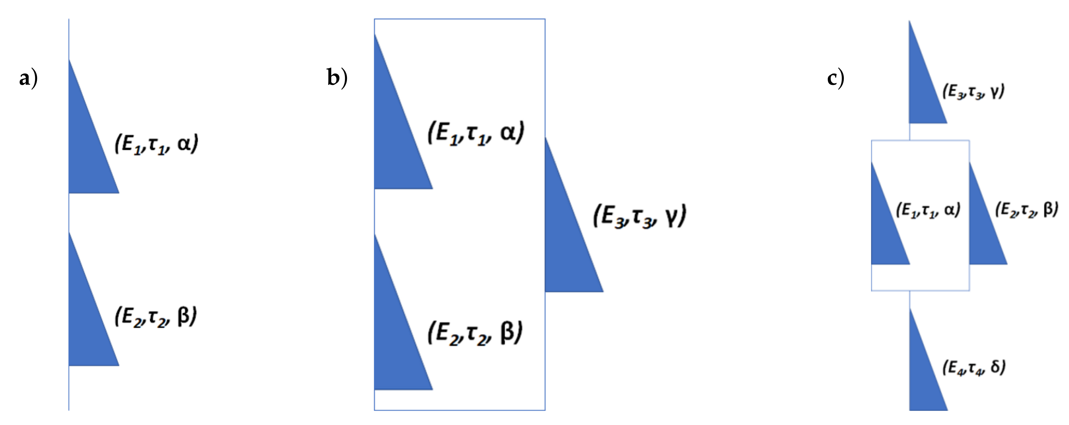
Finally, if we examine Figure 2, simple-to-complex approach in constructing fractional viscoelastic models can be restored. All the models are constructed via connecting fractional elements in series/ parallel. For instance, fractional Zener model is readily obtained from Maxwell one via adding fractional element in parallel. More complex models can be built in a similar fashion. Fractional Burgers model, for example, can be obtained from fractional Kelvin-Voigt one, as outlined in [1]. Fractional viscoelastic models are principally different from their integer-order counterparts. An increase in the number of fractional elements is made to properly describe the specific class of materials. For integer-order models, adding more elements often serves to increase model accuracy. Thus, fractional viscoelastic models not only help to describe behaviors missed by integer-order ones but also simplify problem solving and material characterization.

4. Conclusions

This study has provided detailed parametric analysis of velocity and stress profiles for three fractional viscoelastic models, namely Maxwell model, Zener model, and Burgers model. These models were chosen to represent two-, three-, and four-element viscoelastic systems. Two types of parameters were considered: fractional and elastic. We have extended 2D projections of velocity and stress profiles studied in [1] and considered 3D dynamic velocity and stress surfaces in space and frequency domains. It allowed better visual representation of quantities studied. Surface plots simplified comparison of contributions made by varying individual fractional orders for each model considered. Dependent on researchers’ needs, proper altering of fractional and elastic parameters can be made. Whether achieving of local/global minimum/maximum is required for practical applications, an optimal operating regime can found and visualized. In case the predictions of fractional models should be compared with classical or Newtonian ones, we have provided corresponding constitutive equations.
Fractional Maxwell model was found to be dependent on a pair ( α , β ) of fractional parameters only. The model has demonstrated dynamic behavior with fixed one and varying another fractional parameter, switching from a combination of parabolic and oscillatory behaviors (for lower values of fractional parameters) to purely classic parabolic behavior for the velocity profile (for higher values of fractional parameters). The latter took place only when both tended to unity that corresponded to Newtonian fluid. Fractional Zener model was found to be dependent on three fractional parameters and one elastic parameter. Among these four parameters, the strongest impact is made by the elastic one. As for varying fractional orders, the strongest effect (profile switching rate) was caused by γ , while the weakest by α . Moreover, for all combinations of upper limits for fractional orders, only parabolic profiles were observed. Fractional parameters were found to be proportional to the “rate” of switching between parabolic+oscillating and parabolic profile as well as determining the position of the dominant resonant peak in frequency domain. Fractional Burgers model was defined by four fractional parameters and one elastic parameter. As changing various parameter combinations, several distinct profile types have been obtained. When elastic parameter was fixed, combinations of three fractional parameters set to lower limit with fourth varying resulted in a combination of parabolic and complex resonant (with plateaus) components of varying amplitudes. No switching to purely parabolic profiles was observed. In contrast to it, when three out of four fractional parameters were set to their upper limits, velocity profiles appeared to be purely parabolic with amplitudes decreasing with fractional orders α and β increasing. At the same time, peak amplitudes grew monotonically in a frequency domain. When fractional parameters γ and δ varied, the shape of the parabolic profile changed. More specifically, in a frequency domain it demonstrated a presence of resonant peak followed by decay and finally reaching a nearly constant value. For changing elastic parameter, new types of velocity profiles emerged. In particular, setting fractional orders to lower limits resulted in a series of changing profiles. It started with a combination of parabolic profile, inclined decaying oscillations that were symmetric with respect to pipe centerline. The latter enclosed a plateau. Next, it transformed to parabolic+oscillatory profile. Further increase in ψ resulted in parabolic profile with resonance at certain ω ˜ . We ended up with a simple parabolic profile with the amplitude increasing with ω ˜ . For upper limit values of fractional parameters, a dynamic combination of parabolic and M-shape profile was obtained.
Stress profiles for all three models exhibited three types of behavior. These were aperiodic oscillations in spatial and frequency domains and V-shape profiles (curved or straight). Individual features of the stress profiles, however, varied from model to model. In particular, for fractional Maxwell model the stress profiles changed dynamically with the fractional parameters. More specifically, an increase in fractional parameters resulted in switching from aperiodic oscillations to V-shape profile. For fractional Zener model, two types of behavior were obtained: switching and complete independence from fractional parameters. Stress profiles independent from fractional parameters corresponded to “classic” case. Finally, for fractional Burgers model all three types of profiles were obtained. Different from fractional Zener model, however, here V-shape profiles were observed for both lower and upper limits of fractional orders.
The variety of profile shapes and its dynamics clearly demonstrates how powerful the approach developed is. It is applicable for completely different materials in a wide range of viscous and elastic properties. Dependent on the material used, an appropriate model can be chosen for more accurate predication of viscoelastic pipe flow dynamics. The beauty of the approach developed is that it provides analytical generalization of several most commonly used viscoelastic models as well as clearly demonstrates how rich and complex flow dynamics is when applying fractional calculus methods.
The methods developed in this study not only allow representation of different viscoelastic models in a similar functional form but also relate purely mathematical quantities with that measured experimentally. Thus, theoretical considerations appear to be on a venue of immediate practical applications.

Supplementary Materials

The following are available online at https://www.mdpi.com/2076-3417/10/24/9080/s1.

Author Contributions

Conceptualization, D.G. and R.P.; methodology, D.G.; software, D.G.; validation, R.P.; formal analysis, D.G.; investigation, D.G.; resources, R.P.; writing—original draft preparation, D.G.; writing—review and editing, R.P.; funding acquisition, R.P. All authors have read and agreed to the published version of the manuscript.

Funding

This research was funded by Argonne National Laboratory through grant #ANL 4J-303061-0030A “Multiscale modeling of complex flows”.

Conflicts of Interest

The authors declare no conflict of interest.

References

  1. Gritsenko, D.; Paoli, R. Theoretical analysis of fractional viscoelastic flow in circular pipes: General solutions. Appl. Sci. 2020, 1, 5. [Google Scholar] [CrossRef]
  2. Sun, H.; Zhang, Y.; Baleanu, D.; Chen, W.; Chen, Y. A new collection of real world applications of fractional calculus in science and engineering. Commun. Nonlinear Sci. Numer. Simul. 2018, 64, 213–231. [Google Scholar] [CrossRef]
  3. Atanacković, T.M.; Janev, M.; Pilipović, S. On the thermodynamical restrictions in isothermal deformations of fractional Burgers model. Philos. Trans. R. Soc. A 2020, 378, 20190278. [Google Scholar] [CrossRef]
  4. Chen, R.; Wei, X.; Liu, F.; Anh, V.V. Multi-term time fractional diffusion equations and novel parameter estimation techniques for chloride ions sub-diffusion in reinforced concrete. Philos. Trans. R. Soc. A 2020, 378, 20190538. [Google Scholar] [CrossRef]
  5. Li, S.N.; Cao, B.Y. Fractional-order heat conduction models from generalized Boltzmann transport equation. Philos. Trans. R. Soc. A 2020, 378, 20190280. [Google Scholar] [CrossRef] [PubMed]
  6. Bologna, E.; Di Paola, M.; Dayal, K.; Deseri, L.; Zingales, M. Fractional-order nonlinear hereditariness of tendons and ligaments of the human knee. Philos. Trans. R. Soc. A 2020, 378, 20190294. [Google Scholar] [CrossRef] [PubMed]
  7. Chugunov, V.; Fomin, S. Effect of adsorption, radioactive decay and fractal structure of matrix on solute transport in fracture. Philos. Trans. R. Soc. A 2020, 378, 20190283. [Google Scholar] [CrossRef] [PubMed]
  8. Failla, G.; Zingales, M. Advanced Materials Modelling via Fractional Calculus: Challenges And Perspectives. Philos. Trans. R. Soc. A 2020, 378, 20200050. [Google Scholar] [CrossRef]
  9. Fang, C.; Shen, X.; He, K.; Yin, C.; Li, S.; Chen, X.; Sun, H. Application of fractional calculus methods to viscoelastic behaviours of solid propellants. Philos. Trans. R. Soc. A 2020, 378, 20190291. [Google Scholar] [CrossRef]
  10. Ionescu, C.M.; Birs, I.R.; Copot, D.; Muresan, C.; Caponetto, R. Mathematical modelling with experimental validation of viscoelastic properties in non-Newtonian fluids. Philos. Trans. R. Soc. A 2020, 378, 20190284. [Google Scholar] [CrossRef]
  11. Li, J.; Ostoja-Starzewski, M. Thermo-poromechanics of fractal media. Philos. Trans. R. Soc. A 2020, 378, 20190288. [Google Scholar] [CrossRef] [PubMed]
  12. Tenreiro Machado, J.; Lopes, A.M.; de Camposinhos, R. Fractional-order modelling of epoxy resin. Philos. Trans. R. Soc. A 2020, 378, 20190292. [Google Scholar] [CrossRef] [PubMed]
  13. Di Paola, M.; Alotta, G.; Burlon, A.; Failla, G. A novel approach to nonlinear variable-order fractional viscoelasticity. Philos. Trans. R. Soc. A 2020, 378, 20190296. [Google Scholar] [CrossRef] [PubMed]
  14. Patnaik, S.; Hollkamp, J.P.; Semperlotti, F. Applications of variable-order fractional operators: A review. Proc. R. Soc. A 2020, 476, 20190498. [Google Scholar] [CrossRef] [PubMed] [Green Version]
  15. Patnaik, S.; Semperlotti, F. Variable-order particle dynamics: Formulation and application to the simulation of edge dislocations. Philos. Trans. R. Soc. A 2020, 378, 20190290. [Google Scholar] [CrossRef] [PubMed]
  16. Povstenko, Y.; Kyrylych, T. Fractional thermoelasticity problem for an infinite solid with a penny-shaped crack under prescribed heat flux across its surfaces. Philos. Trans. R. Soc. A 2020, 378, 20190289. [Google Scholar] [CrossRef]
  17. Zhang, X.; Ostoja-Starzewski, M. Impact force and moment problems on random mass density fields with fractal and Hurst effects. Philos. Trans. R. Soc. A 2020, 378, 20190591. [Google Scholar] [CrossRef]
  18. Zorica, D.; Oparnica, L. Energy dissipation for hereditary and energy conservation for non-local fractional wave equations. Philos. Trans. R. Soc. A 2020, 378, 20190295. [Google Scholar] [CrossRef]
  19. Bagley, R.L.; Torvik, P. A theoretical basis for the application of fractional calculus to viscoelasticity. J. Rheol. 1983, 27, 201–210. [Google Scholar] [CrossRef]
  20. Yin, Y.; Zhu, K.Q. Oscillating flow of a viscoelastic fluid in a pipe with the fractional Maxwell model. Appl. Math. Comput. 2006, 173, 231–242. [Google Scholar] [CrossRef]
  21. Shah, S.H.A.M.; Qi, H. Starting solutions for a viscoelastic fluid with fractional Burgers’ model in an annular pipe. Nonlinear Anal. Real World Appl. 2010, 11, 547–554. [Google Scholar] [CrossRef]
  22. Schiessel, H.; Metzler, R.; Blumen, A.; Nonnenmacher, T. Generalized viscoelastic models: Their fractional equations with solutions. J. Phys. A Math. Gen. 1995, 28, 6567. [Google Scholar] [CrossRef]
  23. Friedrich, C.; Schiessel, H.; Blumen, A. Constitutive behavior modeling and fractional derivatives. In Rheology Series; Elsevier: Amsterdam, The Netherlands, 1999; Volume 8, pp. 429–466. [Google Scholar]
Figure 1. Domain definition for circular pipe.
Applsci 10 09080 g001
Figure 2. Fractional viscoelastic models: (a) Maxwell; (b) Zener; (c) Burgers.
Applsci 10 09080 g002
Table 1. Fractional models and their parameters.
Parameter ξ 2 α β γ δ
Model
Fractional Maxwell ρ ω 2 / E 1 ( i ω τ ) α + 1 ( i ω τ ) β [ 0 , 1 ] [ 0 , 1 ]
Fractional Zener ρ ω 2 / E 1 ( E 0 / E ) ( i ω τ ) γ + ( i ω τ ) α + β ( i ω τ ) α + ( i ω τ ) β [ 0 , 1 ] [ 0 , 1 ] [ 0 , 1 ]
Fractional Burgers ρ ω 2 / E 1 ( E 0 / E ) ( i ω τ ) γ + ( i ω τ ) δ + 1 ( i ω τ ) α + ( i ω τ ) β [ 0 , 1 ] [ 1 , 2 ] [ 0 , 1 ] [ 0 , 1 ]
Publisher’s Note: MDPI stays neutral with regard to jurisdictional claims in published maps and institutional affiliations.

