Stability Numbers for Unsupported Conical Excavations in Multi-Layered Cohesive Soils

Abstract

This paper presents the results of a numerical analysis into undrained stability of conical excavation in multi-layered clays. Stability predictions for a wide range of geometric and material combinations are calculated by finite element analyses. The results from the present analysis are expressed in the familiar form of stability numbers reflecting the effect of (1) angle of inclination, (2) depth ratio, which is relative top layer thickness to excavation depth, (3) strength difference between two layers on the rigid base, (4) width ratio, which is excavation height to radius at the bottom of excavation, and (5) thickness ratio, which is the ratio of the excavation height to thickness of soil 1 layers. The obtained stability numbers are compared with existing solutions published in the literature. The failure mechanism in multi-layered clays are also discussed in terms of the displacement pattern.

1. Introduction

The unsupported excavations are commonly encountered in civil engineering projects. Slope instability failures pose serious threat to structures, as these failures may lead to great loss of lives and property [1]. Predicting the stability of excavation is an important task for geotechnical engineers. The combined effects of geology, hydrology, and soil properties generally exist as stability issues.

In order to design the excavation, more rigorous numerical modeling is needed, especially for large-scale complex projects. However, the performing numerical simulations are not always warranted or feasible because of time and cost constraints [2]. Therefore, stability numbers can be seen as convenient tools that provide an easier way to determine the factor of safety.

The stability numbers (N) were used extensively as design tools, and draw the attention of many investigators. The first set of stability number was proposed by Taylor [3] and various stability charts have been developed [4,5,6,7,8,9,10,11]. Traditionally, majority of research have studied the stability number by using the limit-equilibrium method (LEM), which is one of the most popular methods to assess the slope stability [12,13,14]. It is known that for the LEM not only the potential slip surface must be assumed before calculating the factor of safety, but also it cannot guarantee the best solutions [15]. It was found that the factor of safety, which is calculated by LEM, is overestimating compared with the other method [16] and using the finite-element method (FEM) can avoid this drawback, as the failure mechanism is generated automatically [17,18]. With the finite-element method it is generally possible to model many complex conditions with a high degree of realism, including in the analyses, such as things as nonlinear stress–strain behavior, non-homogeneous conditions, and changes in geometry during construction of an excavation [19].

The finite element method has been widely used to simulate excavation construction steps (e.g., [20,21,22]). In a few research [5,9], FEM was used to perform stability charts by using FEM, and only limited parameters such as angle of inclination, the depth ratio, width ratio, which consists of a height, and a radius at the bottom of excavation was considered. In particular, majority of studies have studied homogenous soil. Therefore, various charts based on different valuable parameters such as a strength difference between two layers, relative to the top layer thickness in multi-layer is needed.

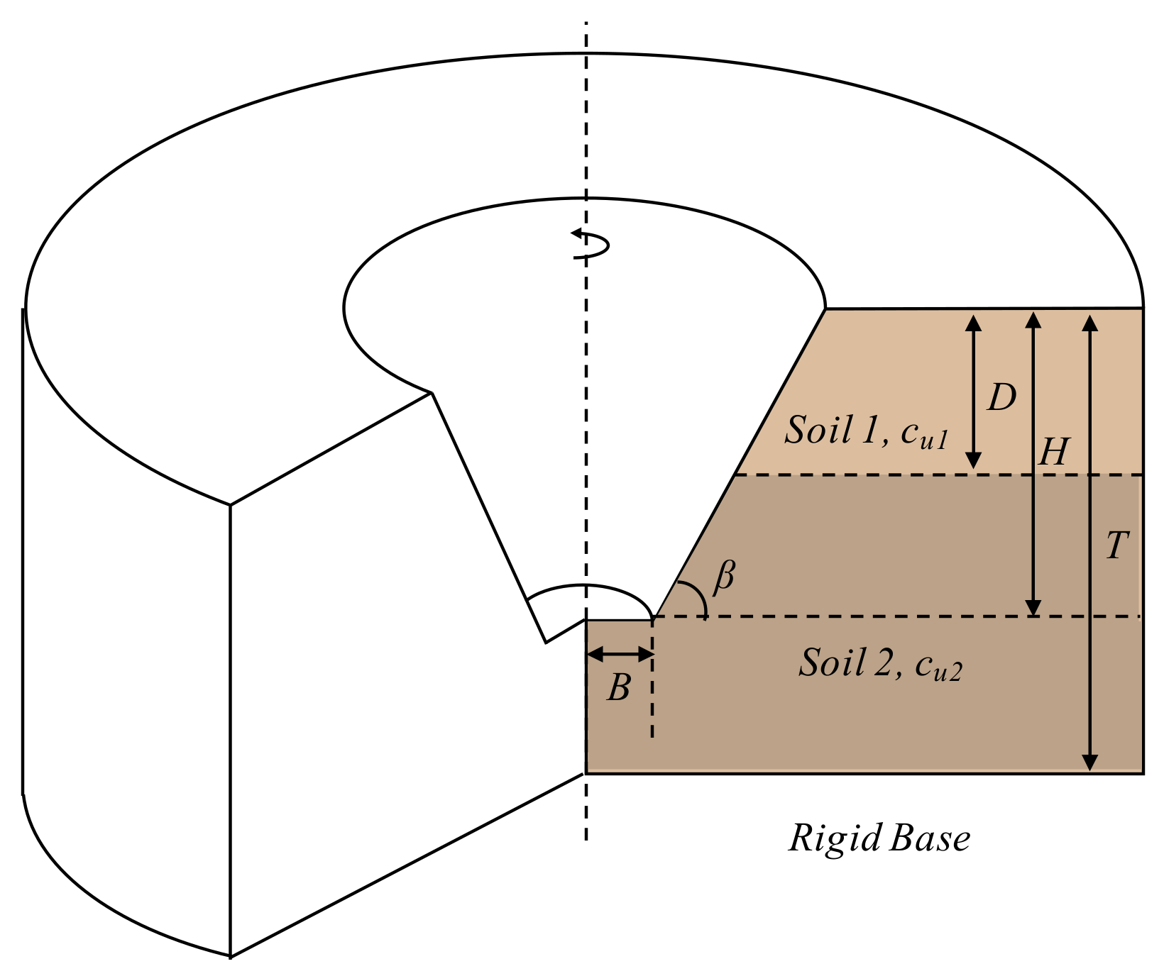
In this study, a series of numerical studies were conducted to assess the variation of the stability number in the multi-layer using FEM. The valuable parameters, which are (1) angle of inclination (β), (2) depth ratio (D/H), which is relative to the top layer thickness to excavation depth, (3) strength ratio (c_u1/c_u2), which is strength difference between two different layers on the rigid base, (4) width ratio (H/B), which is the excavation height to radius at the bottom of excavation, and (5) thickness ratio (T/H), which is the ratio of the excavation height to thickness of soil layers, are considered to confirm the stability. The stability number (N) was provided as a function of these parameters. The obtained stability numbers are compared with existing solutions published in the literature [5,6]. The analysis results are in good agreement with published data. The stability numbers in variable conditions are presented using chart solutions. This chart shows the trend of stability number according to parameters and it can be used for engineering practice.

2. Materials and Methods

2.1. Problem Definition

Griffith and Yu [5] identified the failure regions, which are deep circle, base circle, toe circle, and slope circle by using the finite-element method (FEM). The deep circle is defined that the critical failure surface outcrops to the outside of the toe, but does not reach the strong layer below. The base circle is defined that the critical failure surfaces are base circles and tangent to the strong layer below. The strong layer starts to influence the stability number (N) causing it to rise gradually as the depth ratio is reduced. The toe circle is defined as the critical circles that all pass through the toe and are tangent to the strong layer below. The slope circles are defined as the critical circles outcrop on the slope and are tangent to the strong layer.

Figure 1 shows the different types of critical failure circles. Figure 1a shows the deep circle failure surface, Figure 1b shows the base circle, which is tangent to the strong layer below, Figure 1c shows a toe circle in which the critical circles all pass through the toe and are tangent to the strong layer below, and Figure 1d shows the slope circle, which is the critical circles outcrop on the slope and is tangent to the strong layer.

The soil layers can be more varied at the excavation. Figure 2 shows the case with two layers on a rigid base. Figure 2a shows the case where the top soil layer was smaller than the excavation depth. Figure 2b shows when excavation depth was located on the boundary of two layers. Figure 2c shows the case where the boundary of two layers was behind the excavation depth.

The problem definition is shown in Figure 3, where (1) H is the excavation depth, (2) B is the radius of circular excavation, (3) T is the thickness of total soil layers, (4) D is the depth of the relative top soil layer, and (5) β is the angle of inclination.

The geometry analyzed with two purely cohesive layered soils, where H/B is the width ratio, which is the excavation height to radius at the bottom of excavation, T/H is the thickness ratio, which is the ratio of the excavation height to the thickness of soil layer ratio of the thickness of total soil layers to excavation depth, D/H is the depth ratio, which is relative top layer thickness to excavation depth, c_u1/c_u2 is the strength ratio, which is the top layer strength to second layer strength, and β is the angle of inclination. In order to assess the variation of the stability number (N) the valuable parameters (H/B, T/H, D/H, c_u1/c_u2, and β) were changed.

The variation of parameters is summarized in

Table 1. The range of the parameters studied.

Parameters	Symbol	Values
Width ratio	H/B	0.5, 1, 2, 3, 4, 5, 6 7, 8, 9, 10
Thickness ratio	T/H	1, 1.2, 1.4, 1.6, 1.8, 2.0, 2.2, 3
Depth ratio	D/H	0.25, 0.5, 0.75, 1, 1.25, 1.5, 2
Strength ratio	cu1/cu2	0.25, 0.5, 0.75, 1, 1.25, 1.5, 2, 3, 4, 5
Angle of inclination	β (°)	15, 30, 45, 60

.

The stability numbers are needed as convenient tools that provide an easier way to determine the factor of safety for an excavation. The stability number (N) is significantly affected by the angle of inclination, slope height and thickness of total soil layer [23].

The stability number N is proportional to the factor of safety (FS) as shown in Equation (1)

$$FS=N\frac{\rho }{\gamma }$$

(1)

where ρ is the gradient of strength increase with depth z and γ is the saturated unit weight.

Hunter and Schuster [23] introduced a dimensionless strength gradient parameter M, defined as

$$M=\frac{c_{u0}}{\rho H}$$

(2)

where, c_u0 is the strength at the crest level (z = 0), ρ is the gradient of strength increase with depth z, and H is the slope height (or excavation depth).

In this study, the special case of M = 2 was considered to show that the stability number N depends only on geometry and simplifies the problem.

2.2. Finite Element Model

Two dimensional small-strain finite-element (FE) analysis with axis-symmetry were conducted to predict the stability of excavation for a wide range of geometric and material combinations. All analyses were conducted using the commercial software PLAXIS 2D [24]. The typical 2D mesh and boundary conditions are shown in Figure 4. The soil was modeled with fifteen-node triangular elements. The outer boundary of the mesh was fixed against displacements and the axis-symmetric boundary was adapted to simulate the conical excavation. The soil was modeled as a linearly elastic-perfectly plastic material given by the Mohr–Coulomb criterion. The gravitational acceleration was used to the only load condition.

In the finite-element analysis, the strength reduction method (SRM) was used to estimate and obtain the factor of safety [25,26]. The strength reduction method (SRM) was used to obtain its factor of safety. The strength reduction procedure is defined as follows:

$$c=\frac{c_0}{SRF}$$

(3)

where, c₀ is the original cohesion and shear strength reduction (SRF) is the trial strength reduction factor.

We begin with initial SRF for the initial failure envelope based on c₀ that will not cause failure. The SRF is then iteratively increased, thereby reducing cohesion until the failure envelope intercepts the final failure envelope, which is defined by c_f. At this point the FS is determined by the corresponding SRF.

The factor of safety (FS) is defined as follows:

$$FS=\frac{c_0}{c_{\mathrm{f}}}$$

(4)

where, c₀ is the original cohesion and c_f is the cohesion at failure.

2.3. Validation

To verify the finite element predictions, the numerical results were compared with reported data by Griffiths and Yu [5], and Keawsawasvong and Ukritchon [6]. As shown in Figure 5, the obtained results were in good agreement with the published data. Keawsawasvong and Ukritchon [6] conducted axisymmetric finite element limit analysis for undrained stability of unsupported conical excavations in homogeneous clays. The parametric studies were conducted on the excavated width ratio (H/B) from 0.5 to 10, slope inclinations (β) from 45 to 90°, and dimensionless strength gradients (2bρ/c_u0) from 0 to 4.

In this study, the values defined the dimensionless strength gradients (2bρ/c_u0) as 1 was compared. As shown in Figure 5a, the simulated results were in good agreement with the published data. Griffiths and Yu [5] present the charts that give the stability number as a function of the thickness ratio, strength gradient and slope angle. The numerical analysis was conducted on a thickness ratio (T/H) from 0 to 4, strength gradient (M = c_u0/ρH) from 0.25 to 2, and slope angle (β) from 5 to 60°. When the thickness ratio (T/H) was 1.0 and the strength gradient (M = c_u0/ρH) was 2, the stability number was compared with values of various angles (Figure 5b).

3. Results and Discussion

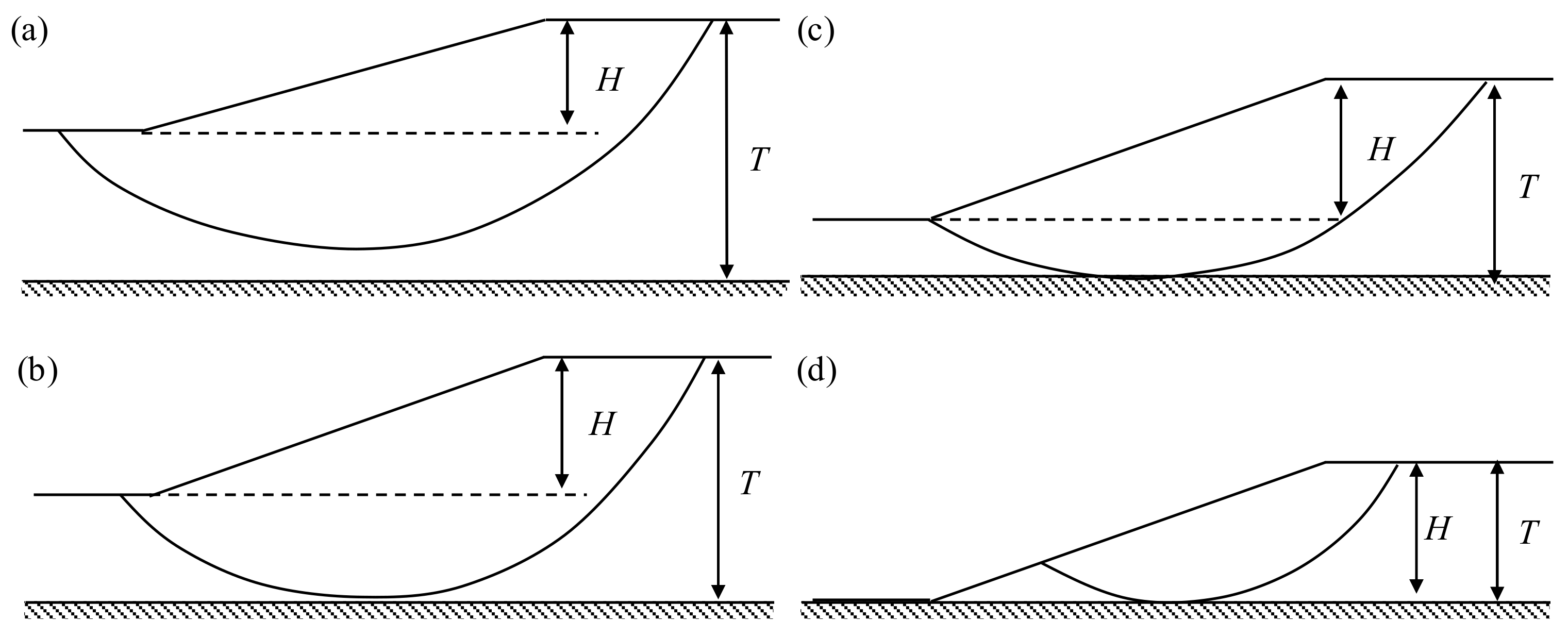
The variation of the stability number (N) for a range of values of the parameters (H/B, T/H, D/H, c_u1/c_u2, and β) was obtained from finite element (FE) analyses. Before showing a full set of results for different parametric combinations, a typical set of graphical results is given to explain the trends of the slip surface.

Figure 6 shows the total deviatoric strain according to the different ranges of the thickness ratio (T/H = 1.2, 1.6, 2.0). All results were performed with only one soil layer on the rigid base. When the excavation surface is closer to the rigid base, the stability number increased due to the slip surface through the rigid base. Griffith and Yu [5] have represented the influence of the thickness ratio (T/H), which is T/H > 2.02 is the deep circle, 2.02 > T/H ≥ 1.54 is the base circle, 1.54 > T/H ≥ 1.37 is the toe circle, and 1.37 > T/H are the slope circles.

As shown in Figure 6, it was confirmed that the slip surface was changed from deep circle to toe circle and stability number (N) was increased as decreasing the thickness ratio. Figure 6a shows the deep circle, which is critical failure surface outcrops to the left of the toe, but is not reached to the strong layer below. Figure 6b shows the base circle, which the slip surface tangent to tangent to the strong layer below. As an influence of the rigid layer, the stability number N was raised. Figure 6c shows the toe circle, which is the slip surface all passes through the toe and is tangent to the rigid layer below.

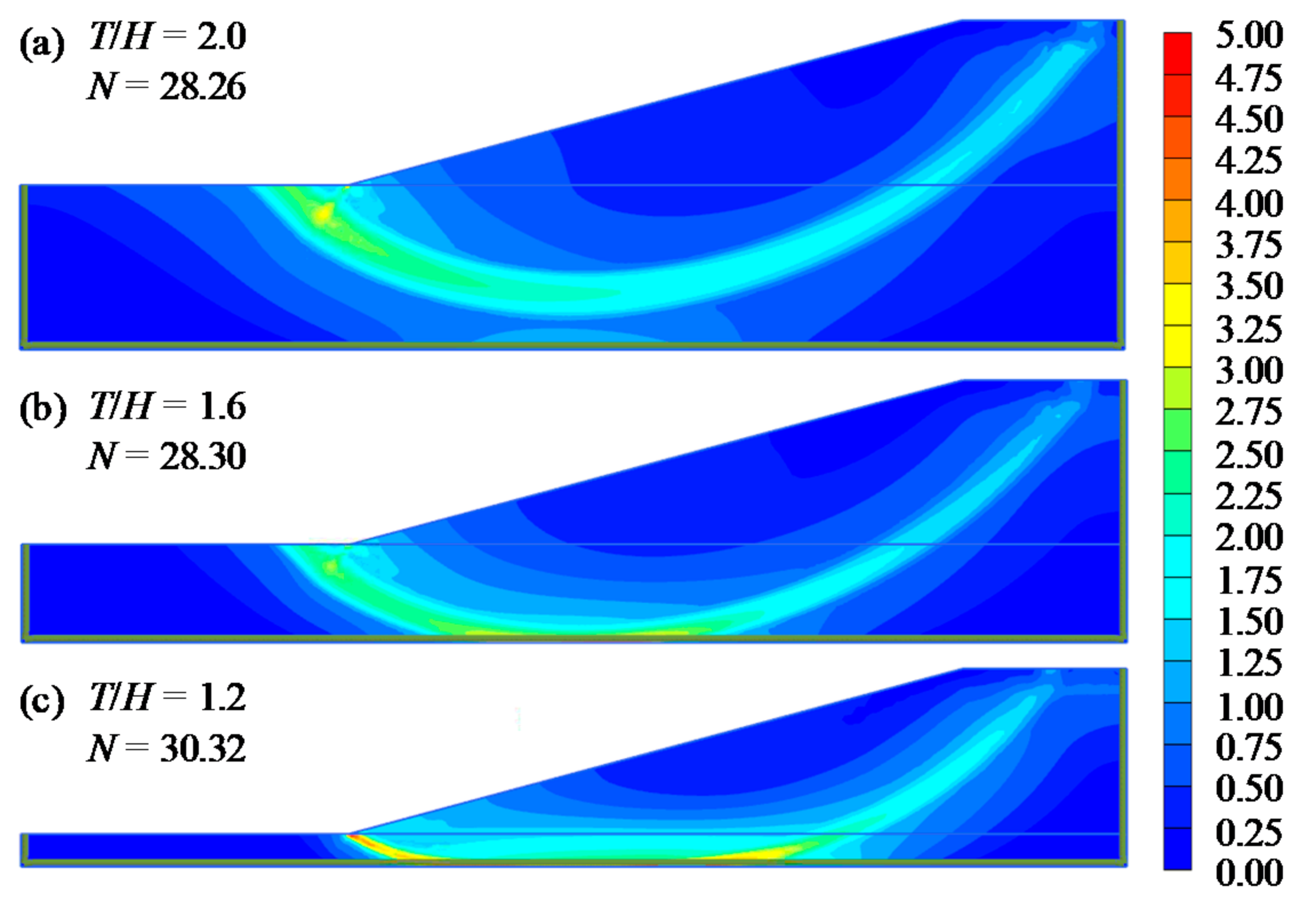
The effect of the width ratio (H/B) is studied by Lyamin and Sloan [27], Keawsawasvong and Ukritchon [6], and Chakraborty and Kumar [28]. The magnitudes of the stability numbers reduce further with decreases in the width ratio (H/B). In order to confirm the effect of width ratio (H/B), which is the excavation height to radius at the bottom of excavation, three cases, which was one soil layer (c_u1/c_u2 = 1.0, D/H = ∞) on the rigid base, were shown in Figure 7. Figure 7a shows the case of the width ratio (H/B) being 0.5, which was a small value. It was represented that the slip surface was a deep circle, which included the entire slip surface due to wide radius of circular excavation. As the width ratio (H/B) increased, the slip surface was affected by the radius of circular excavation (Figure 7b). It was leading to increasing the stability number (Figure 7c).

The geometric parameters such as the width ratio (H/B), depth ratio (D/H) and thickness ratio (T/H) were constant to confirm the effect of angle of inclination (β). Figure 8 shows the effect of angle of inclination (β) in two layers on the rigid base where the strength ratio is (c_u1/c_u2 = 0.25).

Figure 8a shows the shape of the slip surface by the total deviatoric strain in the angle of inclination (β) was 15°. The slip surface was represented by the slope circle, which was the slip surface outcrop on the slope and was tangent to the strong layer due to the c_u1/c_u2 = 0.25, which is the lower layer was relatively strong. As shown in Figure 8b, the shape of slip surface changed to toe circle in β = 30°. Figure 8c shows the shape of the slip surface in β = 45° and Figure 8d shows the shape of the slip surface in β = 60°. It is confirmed that the shape of slip surface changed from the slope circle to the toe circle as the angle of inclination increased.

In order to investigate the effect of the depth ratio (D/H), the typical set (D/H = 0.5, 0.75, 1.00, and 1.25) of results for the case of an excavation with H/B = 0.5, T/H = 2, c_u1/c_u2 = 0.5, and β = 15° was considered. Figure 9 shows the effect of the depth ratio (D/H) in two layers. The slip surface by using the total deviatoric strain was represented according to the depth ratio (D/H) and changing the failure mechanism.

Figure 9a shows the shape of the slip surface by the total deviatoric strain in D/H = 0.5. The slip surface was the base circle. Figure 9b shows the shape of the slip surface, which was both the base circle and deep circle in D/H = 0.75. As shown in Figure 9c, the shape of slip surface was changed to the deep circle in D/H = 1.0. Figure 9d shows the shape of the slip surface, which was the toe circle in D/H = 1.25. It is found that the types of slip surface were changed according to the depth ratio. When c_u1/c_u2 = 0.5, the stability number was decreased as depth ratio was increased.

To examine the effect of the strength difference between two layers, the typical geometry was chosen as T/H = 2, H/B = 0.5, β = 30°, and D/H = 0.75. Figure 10 shows the total deviatoric strain according to strength difference between two layers (c_u1/c_u2). It is revealed that the types of critical failure circles change according to the relative two layers strength. Figure 10a shows the shape of the slip surface which is toe circle on top layer due to the lower layer was relatively strong. As strength ratio (cu1/cu2) increases, it is confirmed that slip surface moves to the lower layer (Figure 10b–d).

The results obtained from the analysis have been presented to give the slope stability numbers. Figure 11 shows the effect of the total thickness of the soil layer to the rigid body and strength difference between two layers on the slope stability number.

Increasing the thickness ratio (T/H) means increasing the thickness of the soil layer to the rigid body at the toe of the slope. Griffiths and Yu [5] showed that as the thickness ratio (T/H) increases in homogeneous soil, the slope stability number gradually decreased and then converged. To confirm the effects of the thickness ratio (T/H), and strength difference between two layers (c_u1/c_u2), the width ratio (H/B) was fixed at 0.5 and depth ratio (D/H) was set to 1. In addition, c_u1 was fixed and c_u2 was changed to change c_u1/c_u2. When c_u1/c_u2 was less than 1, which is c_u2 was greater than c_u1, the stability number had a value similar to T/H = 1 regardless of thickness. When c_u1/c_u2 was greater than or equal to 1, the slope stability number decreased and converged as thickness ratio (T/H) increased, it is similar to the results of Griffiths and Yu [5].

Figure 11a shows the result for β = 15°. When the thickness ratio (T/H) > 1.6, stability number (N) did not change. Figure 11b shows the result for β = 30°. The stability number was reduced and stability number did not change when the thickness ratio (T/H) > 1.4. Figure 11c,d shows the result for β = 45° and β = 60°, respectively. The stability number (N) did not change when the thickness ratio (T/H) > 1.2. Through this, it can be seen that the effect of the thickness ratio (T/H) was larger the lower the slope.

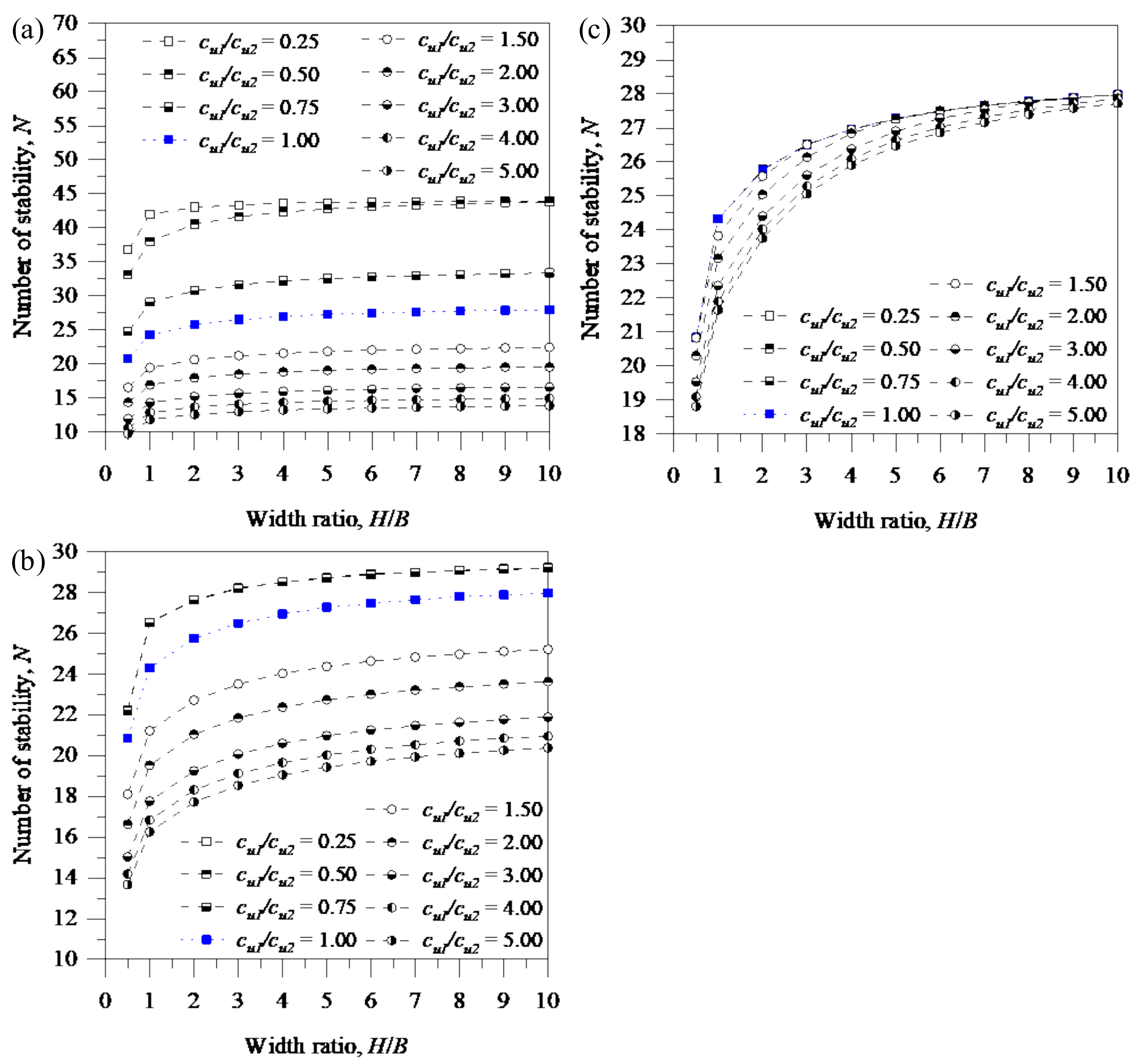
Figure 12 shows the effect of the ratio of excavation height to the radius of the circular excavation ratio (H/B), and strength difference between two layers (c_u1/c_u2) on the slope stability number for a purely two cohesive soil layers on the rigid base. The value of the thickness ratio and angle of inclination was fixed as the thickness ratio (T/H) was 2, and β = 30° to confirm the effects of the width ratio (H/B).

Figure 12a shows the result for D/H = 0.5, which is the top layer thickness was smaller than the excavation depth. The stability number (N) did not change when the width ratio (H/B) was > 5. Figure 12b shows the result for D/H = 1.0, which is the top layer thickness was equal with excavation depth. Figure 12c shows the result for D/H = 1.5, which is the top layer thickness was deeper than excavation depth. It was confirmed that the variation of the stability number was increased as the depth ratio (D/H) increased. However, the effect on the strength ratio (c_u1/c_u2) was reduced as the depth ratio (D/H) increased. As the width ratio (H/B) increased, which is the height of the slope increased or the radius of excavation decreased, the slope stability number increased. This finding can be seen that the sharp increase in H/B < 1. This is because the collapse type changes from deep seated failure to toe failure.

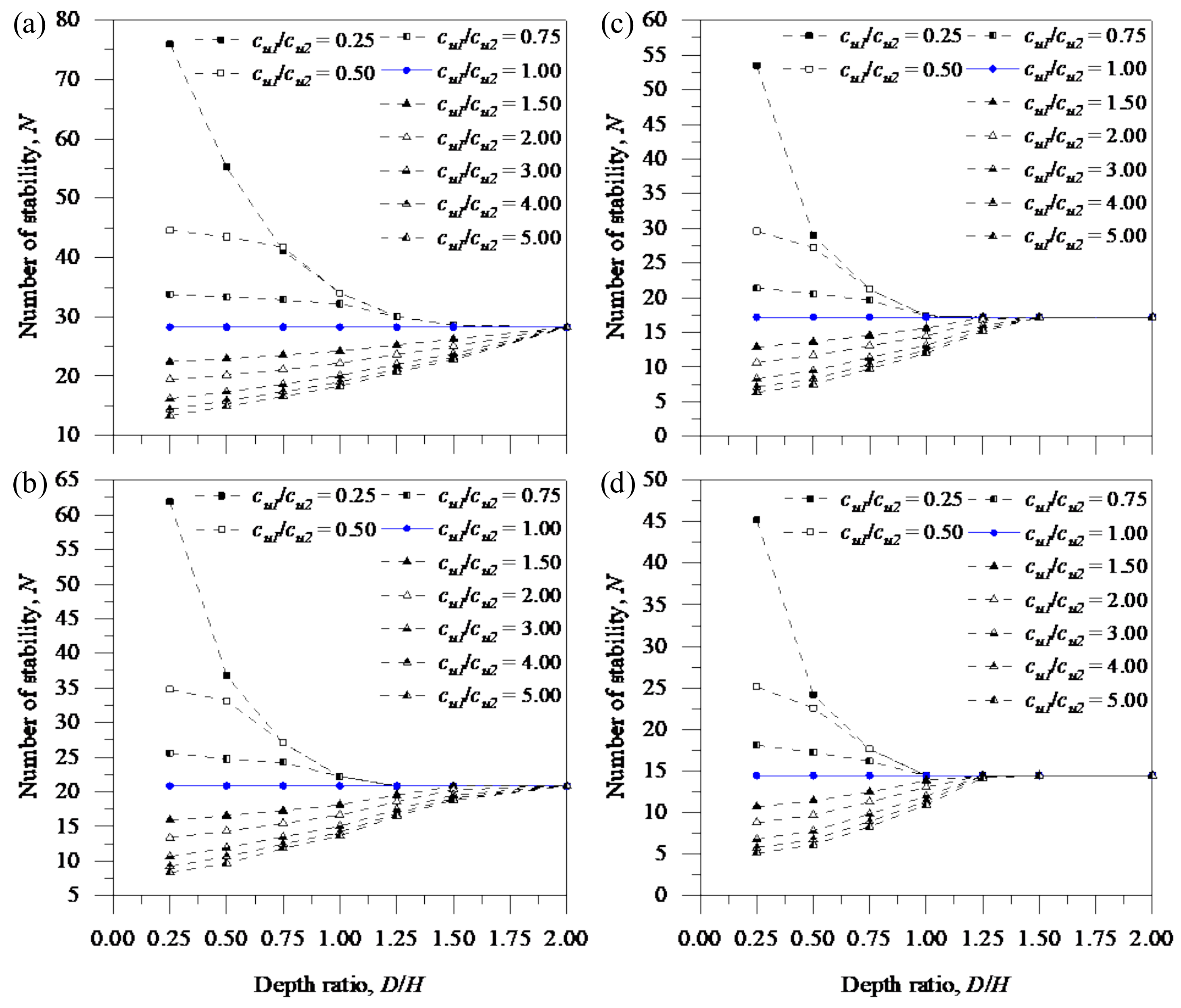
Figure 13 shows the effect of the depth ratio (D/H), which is the relative top layer thickness to excavation depth on the slope stability number. In the multi-layered soil, the relative top layer thickness and strength was a significant influence factor on stability.

Figure 13a shows the stability numbers in β = 15°. The stability number when c_u1/c_u2 < 1 was larger than the stability number when c_u1/c_u2 = 1, which was a homogenous soil layer, but the stability number when c_u1/c_u2 > 1 was smaller than the stability number when c_u1/c_u2 = 1. The variation of stability number was larger as the depth ratio (D/H) was smaller. Figure 13b shows the stability numbers at β = 30°. Figure 13c shows the stability numbers at β = 45°. The stability number was the same with c_u1/c_u2 = 1 when the depth ratio (D/H) > 1.5. Figure 13d shows the stability numbers at β = 60°. The stability number was the same with c_u1/c_u2 = 1 when the depth ratio (D/H) > 1.25. As the angle of inclination increases, the variation of stability number gets small.

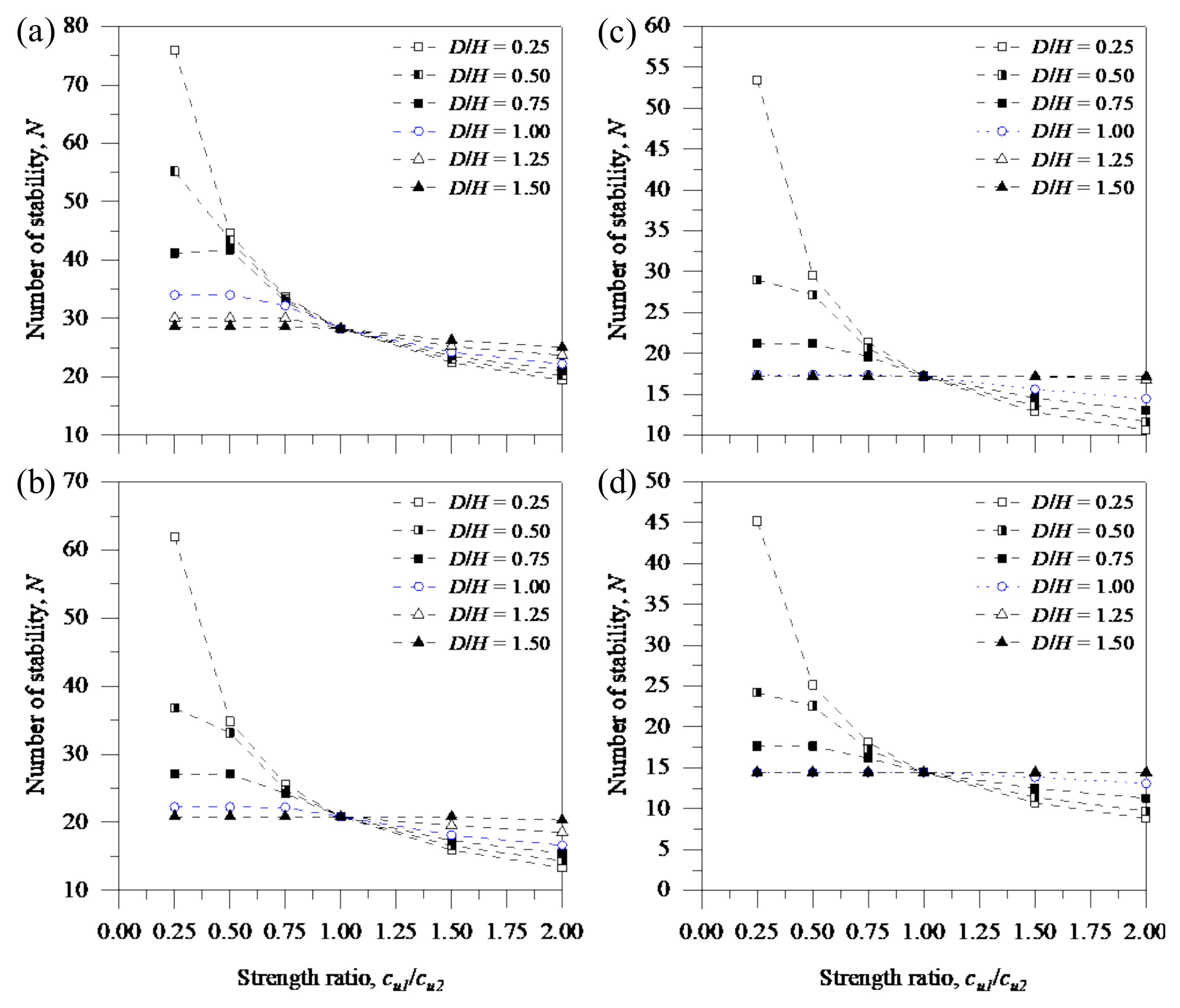
Figure 14 shows the effect of the strength ratio (c_u1/c_u2) which is strength difference between the two layers with the relative top layer thickness to excavation depth. Numerical analyzes were conducted for various slope angle which is β = 15°, β = 30°, β = 45°, and β = 60° with T/H = 2, H/B = 0.5. The strength ratio was defined as c_u1/c_u2 = 0.25, c_u1/c_u2 = 0.50, c_u1/c_u2 = 0.75, c_u1/c_u2 = 1.00, c_u1/c_u2 = 1.25, c_u1/c_u2 = 1.50, and c_u1/c_u2 = 2.0.

Figure 14a shows the stability numbers at β = 15°. When c_u1/c_u2 < 1, the stability number when D/H < 1 was larger than the stability number when D/H = 1, but the stability number when D/H > 1 was smaller than the stability number when D/H = 1. When c_u1/c_u2 > 1, the stability number when D/H < 1 was smaller than the stability number when D/H = 1, but the stability number when D/H > 1 was larger than the stability number when D/H = 1, which is the top layer thickness is equal with excavation depth. Figure 14b shows the stability numbers at β = 30°. Figure 14c shows the stability numbers at β = 45°, and Figure 14d shows the stability numbers at β = 60°. As the angle of slope increases (β = 15° to 60°), the influence of strength ratio (c_u1/c_u2) was decreased.

4. Conclusions

The stability numbers for an unsupported conical excavation in a cohesive soil are generated by using the 2D axis-symmetric FE analysis. The results of the FE analyses were validated by comparing with existing solutions published in the literature for the unsupported stability number. The effects of the slope angle, the strength ratio between two layers, the ratio of the top layer thickness, the width ratio, the excavation height ratio and the depth ratio to stability number were investigated. The results of this research are as follows.

The finite element analysis was conducted to assess the stability of slopes for a wide range of geometric and material combinations. The analysis results are in good agreement with existing solutions published in the literature.

Results were presented for the stability number N as a function of (1) slope inclination, (2) relative top layer thickness, (3) strength difference between two layers, (4) width ratio (excavation height ratio), and (5) depth ratio (ratio of the slope height to thickness of soil layers). The suggested chart for stability number (N) can be used for excavation design in engineering application. It was found that the types of slip surface, which are deep circle, base circle, toe circle, and slope circle could be changed by different parametric combinations.

References

1. Marrapu, B.; Jakka, R.S. Assessment of slope stability using multiple regression analysis. Geomech. Eng. 2017, 13, 237–254. [Google Scholar] [CrossRef]
2. Qian, Z.G.; Li, A.J.; Merifield, R.S.; Lyamin, A.V. Slope Stability Charts for Two-Layered Purely Cohesive Soils Based on Finite-Element Limit Analysis Methods. Int. J. Géoméch. 2015, 15, 06014022. [Google Scholar] [CrossRef]
3. Taylor, D.W. Stability of earth slopes. J. Bost. Soc. Civ. Eng. 1937, 24, 197–246. [Google Scholar]
4. Gens, A.; Hutchinson, J.N.; Cavounidis, S. Three-dimensional analysis of slides in cohesive soils. Géotechnique 1988, 38, 1–23. [Google Scholar] [CrossRef]
5. Griffiths, D.V.; Yu, X. Another look at the stability of slopes with linearly increasing undrained strength. Géotechnique 2015, 65, 824–830. [Google Scholar] [CrossRef]
6. Keawsawasvong, S.; Ukritchon, B. Stability of unsupported conical excavations in non-homogeneous clays. Comput. Geotech. 2017, 81, 125–136. [Google Scholar] [CrossRef]
7. Kim, J.; Salgado, R.; Yu, H.S. Limit Analysis of Soil Slopes Subjected to Pore-Water Pressures. J. Geotech. Geoenviron. Eng. 1999, 125, 49–58. [Google Scholar] [CrossRef]
8. Kumar, J.; Samui, P. Stability determination for layered soil slopes using the upper bound limit analysis. Geotech. Geol. Eng. 2006, 24, 1803–1819. [Google Scholar] [CrossRef]
9. Li, X. Finite element analysis of slope stability using a nonlinear failure criterion. Comput. Geotech. 2007, 34, 127–136. [Google Scholar] [CrossRef]
10. Michalowski, R.L. Stability Charts for Uniform Slopes. J. Geotech. Geoenviron. Eng. 2002, 128, 351–355. [Google Scholar] [CrossRef]
11. Yu, H.S.; Salgado, R.; Sloan, S.W.; Kim, J.M. Limit analysis versus limit equilibrium for slope stability. J. Geotech. Geoenviron. Eng. 1998, 124, 1–11. [Google Scholar] [CrossRef]
12. Bishop, A.W. The use of the Slip Circle in the Stability Analysis of Slopes. Géotechnique 1955, 5, 7–17. [Google Scholar] [CrossRef]
13. Fredlund, D.G.; Krahn, J. Comparison of slope stability methods of analysis. Can. Geotech. J. 1977, 14, 429–439. [Google Scholar] [CrossRef]
14. Morgenstern, N.R.; Price, V.E. The Analysis of the Stability of General Slip Surfaces. Géotechnique 1965, 15, 79–93. [Google Scholar] [CrossRef]
15. Li, A.; Cassidy, M.J.; Wang, Y.; Merifield, R.S.; Lyamin, A. Parametric Monte Carlo studies of rock slopes based on the Hoek–Brown failure criterion. Comput. Geotech. 2012, 45, 11–18. [Google Scholar] [CrossRef]
16. Li, A.J.; Lyamin, A.; Merifield, R.S. Seismic rock slope stability charts based on limit analysis methods. Comput. Geotech. 2009, 36, 135–148. [Google Scholar] [CrossRef]
17. Krabbenhoft, K.; Lyamin, A.V.; Hjiaj, M.; Sloan, S.W. A new discontinuous upper bound limit analysis formulation. Int. J. Numer. Methods Eng. 2005, 63, 1069–1088. [Google Scholar] [CrossRef]
18. Lyamin, A.V.; Sloan, S.W. Lower bound limit analysis using non-linear programming. Int. J. Numer. Methods Eng. 2002, 55, 573–611. [Google Scholar] [CrossRef]
19. Duncan, J.M. State of the Art: Limit Equilmrium and Finite-Element Analysis of Slopes 8. J. Geotech. Eng. 1996, 122, 577–596. [Google Scholar] [CrossRef]
20. Zheng, G.; Du, Y.; Cheng, X.; Diao, Y.; Deng, X.; Wang, F. Characteristics and prediction methods for tunnel deformations induced by excavations. Géoméch. Eng. 2017, 12, 361–397. [Google Scholar] [CrossRef]
21. Zhang, W.; Zhang, R.; Fu, Y.; Goh, A.T.C.; Zhang, F. 2D and 3D numerical analysis on strut responses due to one-strut failure. Geomech. Eng. 2018, 15, 965–972. [Google Scholar] [CrossRef]
22. Mansouri, H.; Asghari-Kaljahi, E. Two dimensional finite element modeling of Tabriz metro underground station L2-S17 in the marly layers. Geomech. Eng. 2019, 19, 315–327. [Google Scholar] [CrossRef]
23. Hunter, J.H.; Schuster, R.L. Stability of Simple Cuttings in Normally Consolidated Clays. Géotechnique 1968, 18, 372–378. [Google Scholar] [CrossRef]
24. Brinkgreve, R.B.J.; Kumarswamy, S.; Swolfs, W.; Foria, F. PLAXIS Finite Element Code for soil and Rock Analyses. Plaxis 2D. Balkema: Rotterdam, The Netherlands, 2018. [Google Scholar]
25. Griffiths, D.V.; Marquez, R.M. Three-dimensional slope stability analysis by elasto-plastic finite elements. Géotechnique 2007, 57, 537–546. [Google Scholar] [CrossRef] [Green Version]
26. Griffiths, D.V.; Lane, P.A. Slope stability analysis by finite elements. Géotechnique 1999, 49, 387–403. [Google Scholar] [CrossRef]
27. Lyaminz, A.V.; Sloan, S.W. Upper bound limit analysis using linear finite elements and non-linear programming. Int. J. Numer. Anal. Methods Géoméch. 2002, 26, 181–216. [Google Scholar] [CrossRef]
28. Chakraborty, D.; Kumar, J. Stability Numbers for a Vertical Circular Excavation with Surcharge. Proc. Natl. Acad. Sci. India Sect. A Phys. Sci. 2016, 87, 115–123. [Google Scholar] [CrossRef]
Figure 1. Different types of critical failure circles: (a) deep circle, (b) base circle, (c) toe circle, and (d) slope circle (modified from Griffith and Yu [5]).
Applsci 10 08839 g001
Figure 2. A schematic diagram of depth ratio variation (a) D/H < 1, (b) D/H = 1, and (c) D/H > 1.
Applsci 10 08839 g002
Figure 3. Problem notation of an unsupported conical excavation.
Applsci 10 08839 g003
Figure 4. Typical finite element mesh and boundary conditions.
Applsci 10 08839 g004
Figure 5. Comparison with published data (a) comparison with Keawsawasvong and Ukritchon [6] and (b) comparison with Griffiths and Yu [5].
Applsci 10 08839 g005
Figure 6. Total deviatoric strain according to T/H, where H/B = 0.5, cu1/cu2 = 1, β = 15° (a) T/H = 2.0, (b) T/H = 1.6, and (c) T/H = 1.2.
Applsci 10 08839 g006
Figure 7. Total deviatoric strain according to width ratio (H/B), where T/H = 2, cu1/cu2 = 1.0, D/H = ∞, β = 15° (a) H/B = 0.5, (b) H/B = 1.0, and (c) H/B = 2.0.
Applsci 10 08839 g007
Figure 8. Total deviatoric strain according to the angle of inclination, where D/H = 1.0, H/B = 0.5, cu1/cu2 = 0.25, T/H = 2.0, (a) β = 15°, (b) β = 30°, (c) β = 45°, and (d) β = 60°
Applsci 10 08839 g008
Figure 9. Total deviatoric strain according to D/H, where T/H = 2, H/B = 0.5, cu1/cu2 = 0.5, β = 15° (a) D/H = 0.50, (b) D/H = 0.75, (c) D/H = 1.0, and (d) D/H = 1.25.
Applsci 10 08839 g009
Figure 10. Total deviatoric strain according to cu1/cu2, where T/H = 2, H/B = 0.5, β = 30°, D/H = 0.75 (a) cu1/cu2 = 0.25, (b) cu1/cu2 = 0.75, (c) cu1/cu2 = 1.50, and (d) cu1/cu2 = 3.00.
Applsci 10 08839 g010
Figure 11. The effect of thickness of the soil layer to the rigid body at a toe of slope, where D/H = 1, H/B = 0.5, (a) β = 15°, (b) β = 30°, (c) β = 45°, and (d) β = 60°.
Applsci 10 08839 g011
Figure 12. The effect of the width ratio on the stability numbers, where T/H = 2, β = 30°, (a) D/H = 0.5, (b) D/H = 1.0, and (c) D/H = 1.5.
Applsci 10 08839 g012
Figure 13. The effect of the relative top layer thickness, where T/H = 2, H/B = 0.5 (a) β = 15°, (b) β = 30°, (c) β = 45°, and (d) β = 60°.
Applsci 10 08839 g013
Figure 14. The effect of the strength difference between two layers, where T/H = 2, H/B = 0.5 (a) β = 15°, (b) β = 30°, (c) β = 45°, and (d) β = 60°.
Applsci 10 08839 g014