Trajectory/Path-Following Controller Based on Nonlinear Jerk-Level Error Dynamics

Abstract

This study proposes a novel, nonlinear trajectory/path-following controller based on jerk-level error dynamics. Therefore, at first the nonlinear acceleration-based kinematic equations of motion of a dynamic system are differentiated with respect to time to obtain a representation connecting the translation jerk with the (specific) force derivative. Furthermore, the path deviation, i.e., the difference between the planned and the actual path, is formulated as nonlinear error dynamics based on the jerk error. Combining the derived equations of motion with the nonlinear error dynamics as well as employing nonlinear dynamic inversion, a control law can be derived that provides force derivative commands, which may be commanded to an inner loop for trajectory control. This command ensures an increased smoothness and faster reaction time compared to traditional approaches based on a force directly. Furthermore, the nonlinear parts in the error dynamic are feedforward components that improve the general performance due to their physical connection with the real dynamics. The validity and performance of the proposed trajectory/path-following controller are shown in an aircraft-related application example.

Nomenclature

The nomenclature of this study is based upon the following principles and introduced here in concise form. A (relative) position vector is denoted as follows:

$${\left({\overrightarrow{\mathbf{r}}}^{AB}\right)}_C={\left({\overrightarrow{\mathbf{r}}}^B\right)}_C-{\left({\overrightarrow{\mathbf{r}}}^A\right)}_C$$

Here, A and B are the points, while C is the coordinate frame. A velocity is consequently given by

$${\left(\frac{\mathrm{d}}{\mathrm{d}t}\right)}^E{\left({\overrightarrow{\mathbf{r}}}^{AB}\right)}_C={\left({\dot{\overrightarrow{\mathbf{r}}}}_D^{AB}\right)}_C^E={\left({\overrightarrow{\mathbf{v}}}_D^{AB}\right)}_C^E$$

Here, D denotes the kind of the velocity, e.g., kinematic K. Furthermore, the superscript E describes the coordinate frame with respect to whom the time derivative is taken. Then, an acceleration is

$${\left(\frac{\mathrm{d}}{\mathrm{d}t}\right)}^F{\left({\overrightarrow{\mathbf{v}}}_D^{AB}\right)}_C^E={\left({\dot{\overrightarrow{\mathbf{v}}}}_D^{AB}\right)}_C^{EF}={\left({\overrightarrow{\mathbf{a}}}_D^{AB}\right)}_C^{EF}$$

The superscript F depicts the coordinate frame with respect to whom the second time derivative is taken.

After this overview on vectors, the following listing summarizes further symbols and indices used in this study.

$\overrightarrow{\mathbf{a}}$	Linear acceleration vector
$\Delta a_{x,T},\Delta a_{y,T},\Delta a_{z,T}$	Trajectory acceleration deviation in three axes
$\overrightarrow{\alpha }$	Rotation acceleration vector
${\alpha }_K$	Kinematic angle of attack
${\mu }_K,{\gamma }_K,{\chi }_K$	Kinematic trajectory angles
$\Delta \overrightarrow{\mathbf{f}}$	Specific force vector
$\Delta {\mathrm{f}}_{\mathrm{x}},\Delta {\mathrm{f}}_{\mathrm{y}},\Delta {\mathrm{f}}_{\mathrm{z}}$	Specific forces in three axes
$G_{\mathrm{LOES}}\left(s\right)$	Actuator transfer function
g	Gravitational acceleration
$\overrightarrow{\mathbf{𝑗}}$	Jerk vector
$\mathbf{K}$	Controller gain matrix
m	Mass
$\overrightarrow{\nu }$	Nonlinear dynamic inversion pseudocontrol
$\overrightarrow{\omega }$	Rotational velocity vector
${\omega }_0$	Natural frequency
$\varphi ,\theta ,\psi$	Euler angles
$\overrightarrow{\mathbf{r}}$	Position vector
$\Delta x_T,\Delta y_T,\Delta z_T$	Trajectory deviation in three axes
$x_N,y_N,z_N$	Aircraft position in navigation frame (generally: North-East-Down)
s	Laplace transform variable
$\overrightarrow{\mathbf{u}}$	Nonlinear dynamic inversion control vector
$\Delta u_T,\Delta v_T,\Delta w_T$	Trajectory velocity deviation in three axes
$V_K$	Kinematic velocity
$\overrightarrow{\mathbf{v}}$	Linear velocity vector
$\zeta$	Relative damping
$Z_{\alpha }$	Lift force derivative w.r.t. angle of attack
F	Trajectory foot point
K	Kinematic quantity/frame
N	Navigation/inertial frame
O	Aircraft-/Trajectory-fixed North-East-down Frame
R	Aircraft reference point
T	Trajectory frame

Assumptions

The following listing summarizes the assumptions used throughout this study.

A. 1

Dynamic model is a rigid-body, i.e., there is no relative movement/velocity between two points on the body.

A. 2

Quasi-stationary mass distribution, i.e., $\dot{m}\approx 0$.

A. 3

Reference frame is a navigation frame $N$ (e.g., North-East-Down) on a fixed-flat earth (i.e., no influence of earth rotation and ellipsoidal earth shape are considered).

A. 4

Reference point is the center of gravity.

It should be noted that these assumptions are fairly standard in, e.g., aviation or robotics [1], and are only used in this paper for the sake of simplicity. Indeed, the specified assumptions are generally not required for the derivation as well as for the application of the proposed methodology and can thus be relaxed based on the required model fidelity. Thus, they do not imply any loss of generality.

1. Introduction

Trajectory control as well as path-following are important topics in the research and industrial communities among others in, e.g., the fields of mobile robotics [2] and autonomous driving [3]. Research in these areas is mainly concerned with both a high availability of the path generation as well as a high integrity, stability, and accuracy of the trajectory/path-following controller. Especially, the importance of stable trajectory/path-following control is central as it ensures the safety of, e.g., the vehicle’s and robot’s operation.

As a consequence of the increased onboard computation power and the emergence of small aerial vehicles, which should operate in close proximity to, e.g., housing, high accurate path control became of paramount importance in the context of aviation in the previous years as well. An overview on often used algorithms is given in [4,5]: The variety of the applied algorithms ranges from simple geometric approaches to linear and decoupled control law design as well as sophisticated nonlinear control techniques, such as dynamic inversion and backstepping, and even optimal control-based approaches like model predictive control.

Especially, nonlinear control techniques have shown their viability in application as they are able to exploit the full physical capabilities and available control authority of an aircraft, thus ensuring a high availability, integrity, and accuracy of the controller command. Additionally, they provide good interaction with the necessary inner-loop controllers as they can consider their dynamic behavior. Examples comprise backstepping control approaches [6], (nonlinear) adaptive control [7], and nonlinear dynamic inversion [8,9,10].

Considering the application to aircraft trajectory/path-following, the approach presented in [8,10] has proven to be viable due to its modularity and independence of the dynamic model. Additionally, it allows for an independent control of the rigid-body/rotational dynamics in an inner loop by a stabilizing controller. Still, a drawback of the methodology is the fact that it is based on acceleration-level aircraft dynamics and kinematics, and thus produces force commands that the inner loop must directly follow. While this is theoretically possible, the inner-loop dynamics and actuators do not allow for direct changes of forces. Thus, this study proposes an enhancement of the existing trajectory/path-following approach by using jerk instead of acceleration-based dynamics and kinematics. In doing so, the command to the inner loop is a force derivative instead of the force, which allows for consideration of actuator dynamics [11,12] and also yields smoother force commands by construction. A further advantage of the jerk-based control for manned application is that studies suggest an increased passenger comfort by controlling the jerk [13]. In addition, jerk is also a major contributor to the efficiency and this therefore often a minimization objective in robot manipulator path planning [14].

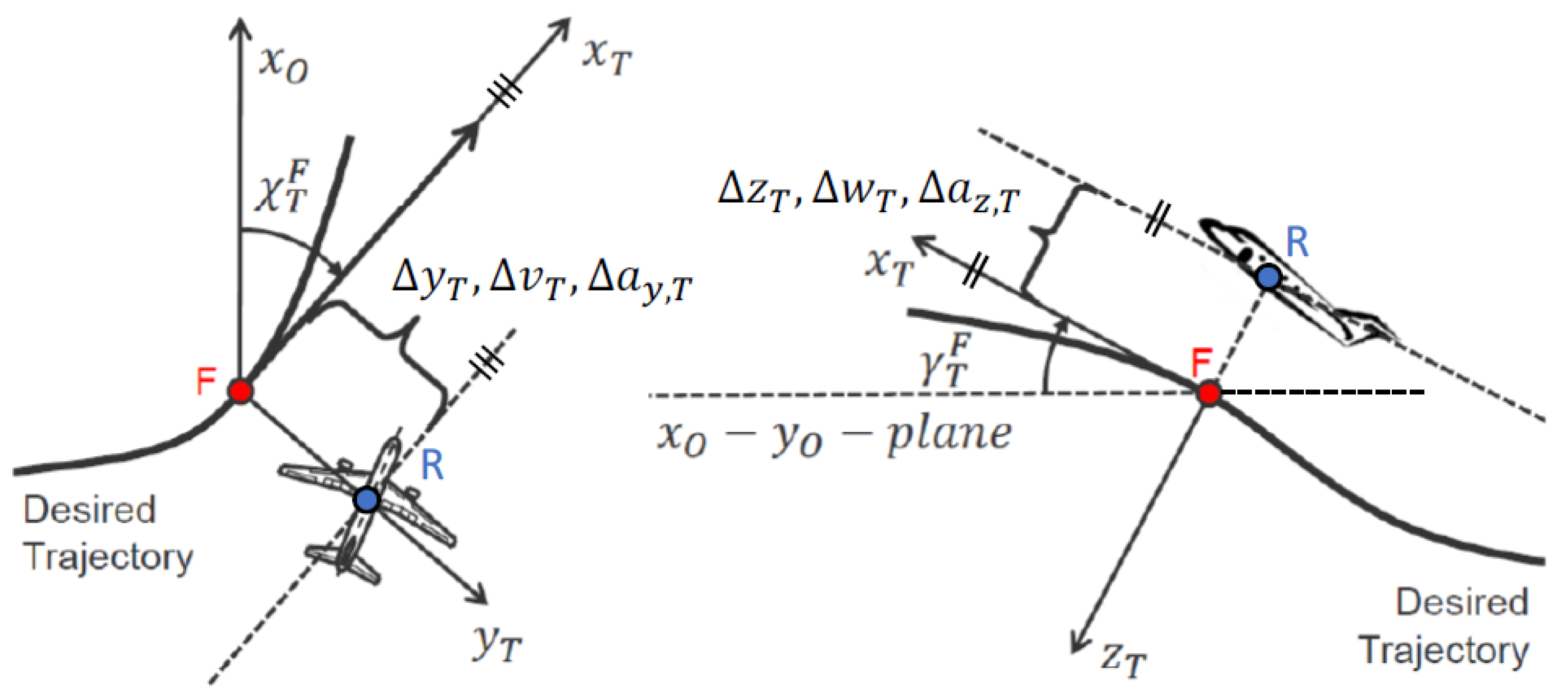
The general idea of the control approach of the paper is depicted in Figure 1: The desired trajectory is generated by a suitable method, e.g., geometric approaches [15,16], (robust) optimal control [17,18,19,20], or shortest path methods [21]. As the aircraft is generally never able to follow the path exactly, either due to imperfect planning or disturbances (e.g, wind or model errors), a deviation between the aircraft reference point $R$ and the trajectory foot point $F$ arises. This point is either specified by a “virtual” aircraft that the actual aircraft “chases” (this is said to be “trajectory control” in this study) [5] or by the orthogonal projection of the aircraft reference point on the trajectory (this is said to be “path-following control” in this study), which may be calculated by the methods proposed in [15,22]. The trajectory/path-following controller then uses these deviations as well as their derivatives (velocity and acceleration) to calculate a suitable control command to reduce them. It should be noted that already by considering acceleration errors, the controller can react faster to deviation than with the acceleration based formulation in [8,10], which only starts acting on velocity errors.

Summarizing, the contributions of this study are as follows.

• Derivation of jerk-level dynamic equations, i.e., a connection between the jerk and the (specific) force derivatives.
• Derivation of nonlinear, jerk-based error dynamics between the reference point of the dynamic model and the desired point (“foot point”) on the trajectory.
• Connection of jerk-based dynamics and kinematics to formulate control law based on nonlinear dynamic inversion.

To achieve this, the study is structured as follows. In Section 2, the kinematic equations of motion are extended to the jerk-level and force derivative. This is used in Section 3 together with the jerk-level error dynamics and nonlinear dynamic inversion to formulate a nonlinear control law. Then, the viability of the approach is illustrated by the example in Section 4. Concluding, Section 5 gives remarks and an outlook on future work.

2. Jerk-Based Dynamic Equations

The derivation of the jerk-based dynamics starts with the acceleration-based kinematic equation of motion using specific forces on a fixed-flat earth (Assumption A.3) [1,10]:

$${\left({\overrightarrow{\mathbf{a}}}_K^R\right)}_K^{NK}+{\left({\overrightarrow{\omega }}_K^{OK}\right)}_K\times {\left({\overrightarrow{\mathbf{v}}}_K^R\right)}_K^N={\left(\Delta {\overrightarrow{\mathbf{f}}}^R\right)}_K$$

(1)

Here, the specific forces ${\left(\Delta {\overrightarrow{\mathbf{f}}}^R\right)}_K={\left[\begin{array}{ccc}\Delta {\mathrm{f}}_{\mathrm{x}}& \Delta {\mathrm{f}}_{\mathrm{y}}& \Delta {\mathrm{f}}_{\mathrm{z}}\end{array}\right]}^{\mathsf{T}}$ are normalized by the mass $m$ of the dynamic system (e.g., aircraft or robot). It should be noted that this is possible due to Assumption A.2, i.e., because the model mass is time-invariant.

To get to the jerk-level and introduce the time derivative of the specific forces, Equation (1) must be differentiated with respect to time in an inertial frame, which is the navigation frame $N$ in this study (Assumptions A.2 and A.3):

$$\underset{{\left({\overrightarrow{\mathbf{𝑗}}}_K^R\right)}_K^{NKN}}{\underbrace{{\left({\dot{\overrightarrow{\mathbf{a}}}}_K^R\right)}_K^{NKN}}}+\underset{{\left({\dot{\overrightarrow{\omega }}}_K^{OK}\right)}_K^N}{\underbrace{{\left({\overrightarrow{\alpha }}_K^{OK}\right)}_K^N}}\times {\left({\overrightarrow{\mathbf{v}}}_K^R\right)}_K^N+{\left({\overrightarrow{\omega }}_K^{OK}\right)}_K\times {\left({\overrightarrow{\mathbf{a}}}_K^R\right)}_K^{NN}={\left({\dot{\Delta \overrightarrow{\mathbf{f}}}}^R\right)}_K^N$$

(2)

Using the Euler differentiation rule [1] and introducing the jerk for the time derivative of the acceleration, Equation (2) results in the following form.

$$\begin{array}{cc}\hfill & \underset{{\left({\overrightarrow{\mathbf{𝑗}}}_K^R\right)}_K^{NKN}}{\underbrace{{\left({\overrightarrow{\mathbf{𝑗}}}_K^R\right)}_K^{NKK}+{\left({\overrightarrow{\omega }}_K^{NK}\right)}_K\times {\left({\overrightarrow{\mathbf{a}}}_K^R\right)}_K^{NK}}}+\underset{{\left({\overrightarrow{\alpha }}_K^{OK}\right)}_K^N}{\underbrace{\left[{\left({\overrightarrow{\alpha }}_K^{OK}\right)}_K^K+{\left({\overrightarrow{\omega }}_K^{NK}\right)}_K\times {\left({\overrightarrow{\omega }}_K^{OK}\right)}_K\right]}}\times {\left({\overrightarrow{\mathbf{v}}}_K^R\right)}_K^N\hfill \\ \hfill +& {\left({\overrightarrow{\omega }}_K^{OK}\right)}_K\times \underset{{\left({\overrightarrow{\mathbf{a}}}_K^R\right)}_K^{NN}}{\underbrace{\left[{\left({\overrightarrow{\mathbf{a}}}_K^R\right)}_K^{NK}+{\left({\overrightarrow{\omega }}_K^{NK}\right)}_K\times {\left({\overrightarrow{\mathbf{v}}}_K^R\right)}_K^N\right]}}=\underset{{\left({\dot{\Delta \overrightarrow{\mathbf{f}}}}^R\right)}_K^N}{\underbrace{{\left({\dot{\Delta \overrightarrow{\mathbf{f}}}}^R\right)}_K^K+{\left({\overrightarrow{\omega }}_K^{NK}\right)}_K\times {\left(\Delta {\overrightarrow{\mathbf{f}}}^R\right)}_K}}\hfill \end{array}$$

(3)

Consequently, Equation (3) provides the desired connection between the jerk ${\left({\overrightarrow{\mathbf{𝑗}}}_K^R\right)}_K^{NKK}$ and the specific force derivative ${\left({\dot{\Delta \overrightarrow{\mathbf{f}}}}^R\right)}_K^K$ that is utilized in Section 3 to the dynamic equation with the nonlinear error dynamics.

3. Nonlinear Error Dynamics and Control Strategy

The error dynamics are derived in the following for the difference between the orthogonal projection of the trajectory foot point and the dynamic model reference point (see Figure 1) [8,10]:

$${\left({\overrightarrow{\mathbf{r}}}^{FR}\right)}_T={\left({\overrightarrow{\mathbf{r}}}^R\right)}_T-{\left({\overrightarrow{\mathbf{r}}}^F\right)}_T={\left[\begin{array}{ccc}\Delta x_T& \Delta y_T& \Delta z_T\end{array}\right]}^{\mathsf{T}}$$

(4)

Based on Equation (4), the velocity deviation can be calculated by deriving Equation (4) with respect to the trajectory frame and applying the Euler differentiation rule (it should be noted that we do not need to derive with respect to an inertial frame in this case, as the position deviation is not based on Newtonian mechanics. Furthermore, the velocity is specified kinematically, and thus has an additional index $K$ added inside the bracket) [8,10]:

$${\left(\frac{\mathrm{d}}{\mathrm{d}t}\right)}^T{\left({\overrightarrow{\mathbf{r}}}^{FR}\right)}_T={\left({\overrightarrow{\mathbf{v}}}_K^{FR}\right)}_T^T={\left[\begin{array}{ccc}\Delta u_T& \Delta v_T& \Delta w_T\end{array}\right]}^{\mathsf{T}}={\left({\overrightarrow{\mathbf{v}}}_K^{FR}\right)}_T^N+{\left({\overrightarrow{\omega }}_K^{TN}\right)}_T\times {\left({\overrightarrow{\mathbf{r}}}^{FR}\right)}_T$$

(5)

Then, the acceleration deviation is consequently given by deriving Equation (5) once more in the trajectory frame as well as applying the Euler differentiation rule to introduce measurable quantities [8,10]:

$$\begin{array}{cc}\hfill {\left({\overrightarrow{\mathbf{a}}}_K^{FR}\right)}_T^{TT}& ={\left[\begin{array}{ccc}\Delta a_{x,T}& \Delta a_{y,T}& \Delta a_{z,T}\end{array}\right]}^{\mathsf{T}}={\displaystyle \underset{{\left({\overrightarrow{\mathbf{a}}}_K^{FR}\right)}_T^{NT}}{\underbrace{\underset{{\left({\overrightarrow{\mathbf{a}}}_K^R\right)}_T^{NT}}{\underbrace{{\left({\overrightarrow{\mathbf{a}}}_K^R\right)}_T^{NK}+{\left({\overrightarrow{\omega }}_K^{TK}\right)}_T\times {\left({\overrightarrow{\mathbf{v}}}_K^R\right)}_T^N}}-{\left({\overrightarrow{\mathbf{a}}}_{\mathrm{des},K}^F\right)}_T^{NT}}}}\hfill \\ \hfill & +{\left({\overrightarrow{\omega }}_K^{TN}\right)}_T\times {\left({\overrightarrow{\mathbf{v}}}_K^{FR}\right)}_T^T+{\left({\overrightarrow{\alpha }}_K^{TN}\right)}_T^T\times {\left({\overrightarrow{\mathbf{r}}}^{FR}\right)}_T\hfill \end{array}$$

(6)

Here, the lead acceleration ${\left({\overrightarrow{\mathbf{a}}}_K^{FR}\right)}_T^{NT}$ is split (see Equation (4)) into the a part with respect to the reference point, ${\left({\overrightarrow{\mathbf{a}}}_K^R\right)}_T^{NT}$, and a part with respect to the foot point (the “desired” acceleration), ${\left({\overrightarrow{\mathbf{a}}}_{\mathrm{des},K}^F\right)}_T^{NT}$. This is used in the following to introduce the dynamic equations from Section 2 into the jerk dynamics derived next. Additionally, the desired acceleration/jerk is an additional design variable in the commanded trajectory specification that can be used to achieve a desired behavior.

Finally, the jerk error can be calculated by deriving Equation (6) one final time with respect to the trajectory frame:

$$\begin{array}{cc}\hfill {\left({\overrightarrow{\mathbf{𝑗}}}_K^{FR}\right)}_T^{TTT}& ={\left({\overrightarrow{\mathbf{𝑗}}}_K^R\right)}_T^{NKT}+{\left({\overrightarrow{\alpha }}_K^{TK}\right)}_T^T\times {\left({\overrightarrow{\mathbf{v}}}_K^R\right)}_T^N+{\left({\overrightarrow{\omega }}_K^{TK}\right)}_T\times {\left({\overrightarrow{\mathbf{a}}}_K^R\right)}_T^{NT}-{\left({\overrightarrow{\mathbf{𝑗}}}_{\mathrm{des},K}^F\right)}_T^{NTT}\hfill \\ \hfill & +{\left({\overrightarrow{\alpha }}_K^{TN}\right)}_T^T\times {\left({\overrightarrow{\mathbf{v}}}_K^{FR}\right)}_T^T+{\left({\overrightarrow{\omega }}_K^{TN}\right)}_T\times {\left({\overrightarrow{\mathbf{a}}}_K^{FR}\right)}_T^{TT}\hfill \\ \hfill & +{\left({\dot{\overrightarrow{\alpha }}}_K^{TN}\right)}_T^{TT}\times {\left({\overrightarrow{\mathbf{r}}}^{FR}\right)}_T+{\left({\overrightarrow{\alpha }}_K^{TN}\right)}_T^T\times {\left({\overrightarrow{\mathbf{v}}}_K^{FR}\right)}_T^T\hfill \end{array}$$

(7)

Now, the Euler differentiation rule may be applied once more to transform the derivatives with respect to the trajectory frame to a more suitable representation for analysis and implementation:

$$\begin{array}{cc}\hfill {\left({\overrightarrow{\mathbf{𝑗}}}_K^{FR}\right)}_T^{TTT}& =\underset{{\left({\overrightarrow{\mathbf{𝑗}}}_K^R\right)}_T^{NKT}}{\underbrace{{\left({\overrightarrow{\mathbf{𝑗}}}_K^R\right)}_T^{NKK}+{\left({\overrightarrow{\omega }}_K^{TK}\right)}_T\times {\left({\overrightarrow{\mathbf{a}}}_K^R\right)}_T^{NK}}}+{\left({\overrightarrow{\alpha }}_K^{TK}\right)}_T^T\times {\left({\overrightarrow{\mathbf{v}}}_K^R\right)}_T^N\hfill \\ \hfill & +{\left({\overrightarrow{\omega }}_K^{TK}\right)}_T\times \underset{{\left({\overrightarrow{\mathbf{a}}}_K^R\right)}_T^{NT}}{\underbrace{\left[{\left({\overrightarrow{\mathbf{a}}}_K^R\right)}_T^{NK}+{\left({\overrightarrow{\omega }}_K^{TK}\right)}_T\times {\left({\overrightarrow{\mathbf{v}}}_K^R\right)}_T^N\right]}}-{\left({\overrightarrow{\mathbf{𝑗}}}_{\mathrm{des},K}^F\right)}_T^{NTT}\hfill \\ \hfill & +{\left({\overrightarrow{\omega }}_K^{TN}\right)}_T\times {\left({\overrightarrow{\mathbf{a}}}_K^{FR}\right)}_T^{TT}+2{\left({\overrightarrow{\alpha }}_K^{TN}\right)}_T^T\times {\left({\overrightarrow{\mathbf{v}}}_K^{FR}\right)}_T^T+{\left({\dot{\overrightarrow{\alpha }}}_K^{TN}\right)}_T^{TT}\times {\left({\overrightarrow{\mathbf{r}}}^{FR}\right)}_T\hfill \end{array}$$

(8)

Thus, the nonlinear jerk-based error dynamics have been derived. It is important to note that Equation (8) shows that the error dynamics are, generally, a linear parameter varying system with respect to the trajectory deviation and its derivatives (last line in Equation (8)). Additionally, the top two lines in Equation (8) depict the nonlinear influence of the dynamic model, while the desired jerk of the foot point (second line) is a design variable of the planned trajectory.

As stated in the sections before, the goal of the trajectory controller is to command the specific force derivatives to the inner-loop controller, which stabilizes the rotational dynamics, utilizing the nonlinear error dynamics in Equation (8). To achieve this, Equation (3) can be solved for the jerk ${\left({\overrightarrow{\mathbf{𝑗}}}_K^R\right)}_T^{NKK}$ (including a transformation from the kinematic $K$ to the trajectory $T$ frame using an orthogonal transformation matrix) and inserted for the first addend in Equation (8):

$$\begin{array}{cc}\hfill \underset{\overrightarrow{\nu }}{\underbrace{{\left({\overrightarrow{\mathbf{𝑗}}}_K^{FR}\right)}_T^{TTT}}}& =\underset{\overrightarrow{\mathbf{u}}}{\underbrace{{\left({\dot{\Delta \overrightarrow{\mathbf{f}}}}^R\right)}_T^K}}+{\left({\overrightarrow{\omega }}_K^{NK}\right)}_T\times {\left(\Delta {\overrightarrow{\mathbf{f}}}^R\right)}_T\hfill \\ \hfill & -{\left({\overrightarrow{\omega }}_K^{NK}\right)}_T\times {\left({\overrightarrow{\mathbf{a}}}_K^R\right)}_T^{NK}-\left[{\left({\overrightarrow{\alpha }}_K^{OK}\right)}_T^K+{\left({\overrightarrow{\omega }}_K^{NK}\right)}_T\times {\left({\overrightarrow{\omega }}_K^{OK}\right)}_T\right]\times {\left({\overrightarrow{\mathbf{v}}}_K^R\right)}_T^N\hfill \\ \hfill & -{\left({\overrightarrow{\omega }}_K^{OK}\right)}_T\times \left[{\left({\overrightarrow{\mathbf{a}}}_K^R\right)}_T^{NK}+{\left({\overrightarrow{\omega }}_K^{NK}\right)}_T\times {\left({\overrightarrow{\mathbf{v}}}_K^R\right)}_T^N\right]+{\left({\overrightarrow{\omega }}_K^{TK}\right)}_T\times {\left({\overrightarrow{\mathbf{a}}}_K^R\right)}_T^{NK}\hfill \\ \hfill & +{\left({\overrightarrow{\alpha }}_K^{TK}\right)}_T^T\times {\left({\overrightarrow{\mathbf{v}}}_K^R\right)}_T^N+{\left({\overrightarrow{\omega }}_K^{TK}\right)}_T\times \left[{\left({\overrightarrow{\mathbf{a}}}_K^R\right)}_T^{NK}+{\left({\overrightarrow{\omega }}_K^{TK}\right)}_T\times {\left({\overrightarrow{\mathbf{v}}}_K^R\right)}_T^N\right]-{\left({\overrightarrow{\mathbf{𝑗}}}_{\mathrm{des},K}^F\right)}_T^{NTT}\hfill \\ \hfill & +{\left({\overrightarrow{\omega }}_K^{TN}\right)}_T\times {\left({\overrightarrow{\mathbf{a}}}_K^{FR}\right)}_T^{TT}+2{\left({\overrightarrow{\alpha }}_K^{TN}\right)}_T^T\times {\left({\overrightarrow{\mathbf{v}}}_K^{FR}\right)}_T^T+{\left({\dot{\overrightarrow{\alpha }}}_K^{TN}\right)}_T^{TT}\times {\left({\overrightarrow{\mathbf{r}}}^{FR}\right)}_T\hfill \end{array}$$

(9)

Here, nonlinear dynamic inversion [1,8,10], i.e.,

$$\overrightarrow{\mathbf{u}}=\overrightarrow{\nu }-\overrightarrow{\mathbf{g}}\left(·\right),$$

(10)

with $\overrightarrow{\mathbf{g}}\left(·\right)$ containing all nonlinear addends from Equation (8) being used to calculate the specific force derivative (command variable $\overrightarrow{\mathbf{u}}$), which may then be commanded to the inner loop. It should be noted that the values in $\overrightarrow{\mathbf{g}}\left(·\right)$ are all available from sensor measurements (e.g., aircraft linear/rotational velocity and acceleration) or can be easily calculated from these (e.g., deviations). For this, all desired (i.e., planned) trajectory related quantities are specified by, e.g., the trajectory generation module and consequently, also known. Thus, Equation (10) can be used to calculate the desired control $\overrightarrow{\mathbf{u}}$ (i.e., the specific force derivative) by solving for it and using the pseudocontrol $\overrightarrow{\nu }$ as an input variable. For this purpose, the pseudocontrol may, e.g., follow a linear error controller law:

$$\overrightarrow{\nu }={\left({\overrightarrow{\mathbf{𝑗}}}_K^{FR}\right)}_T^{TTT}=-{\mathbf{K}}_{\mathrm{p}}·{\left({\overrightarrow{\mathbf{r}}}^{FR}\right)}_T-{\mathbf{K}}_{\mathrm{d}}·{\left({\overrightarrow{\mathbf{v}}}_K^{FR}\right)}_T^T-{\mathbf{K}}_{\mathrm{dd}}·{\left({\overrightarrow{\mathbf{a}}}_K^{FR}\right)}_T^{TT},{\mathbf{K}}_p\succ \mathbf{0},{\mathbf{K}}_d\succ \mathbf{0},{\mathbf{K}}_{dd}\succ \mathbf{0}$$

(11)

Consequently, the pseudocontrol is chosen such that the error between reference and foot point reduces, while following the desired trajectory. The matrices ${\mathbf{K}}_p$, ${\mathbf{K}}_d$, and ${\mathbf{K}}_{dd}$ are positive definite design matrices specified to shape the response characteristics and to ensure the stability of the error dynamics by commanding a stabilizing pseudocontrol. Thus, a proper choice of these matrices ensures not only the stability of the trajectory controller, but also provides disturbance rejection.

It should be noted that the nonlinear error controller in Equations (9)–(11) is derived for the case of trajectory control here. Nonetheless, it is straightforward to apply the methodology to path-following control as well by removing the dependence on $\Delta x_T$ (i.e., not controlling this deviation).

Concluding, the control law based on nonlinear error dynamics has been derived in Equations (9) and (11) using nonlinear dynamic inversion as specified in Equation (10). The applicability is shown in an aircraft-related example in the next section.

4. Illustrative Example

This section gives different test results to show the viability of the proposed control scheme in Section 3. Therefore, Section 4.1 starts with an introduction of the generic simulation model. Then, Section 4.2 investigates the effect of the turn radius on the maximal lateral trajectory deviation, i.e., the effects of the model dynamics including actuators and how the error controller deals with it in a simple setup. Finally, Section 4.3 concludes with an example of the controller in trajectory control mode for a complex trajectory-following task.

4.1. Model Formulation

The model is based on the kinematic equations of motion introduced in Equation (1) with constants defined in

Table 1. Constants used in the simulation model.

Name	Symbol	Value	Unit
Actuator natural frequency	${\omega }_0$	20	$\frac{\mathrm{rad}}{\mathrm{s}}$
Actuator damping	$\zeta$	1	−
Gravitational acceleration	g	$9.81$	$\frac{\mathrm{m}}{{\mathrm{s}}^2}$
Linear force derivative	$Z_{\alpha }$	$-3$	$\frac{1}{\mathrm{s}}$
Position error gain matrix	${\mathbf{K}}_{\mathrm{p}}$	${\mathbf{I}}_{3\times 3}$	−
Velocity error gain matrix	${\mathbf{K}}_{\mathrm{d}}$	$3·{\mathbf{I}}_{3\times 3}$	−
Acceleration error gain matrix	${\mathbf{K}}_{\mathrm{dd}}$	$9·{\mathbf{I}}_{3\times 3}$	−
Aircraft mass	m	100	$\mathrm{kg}$

. To improve the model’s fidelity for real-world applications, a lower order equivalent system transfer function $G_{\mathrm{LOES}}$ is used for course and climb as well as the angle of attack dynamics to mimic a rigid-body behavior, and thus the rotational dynamics. This is defined as follows (in the Laplace domain [1]).

$$\begin{array}{cc}\hfill G_{\mathrm{LOES}}\left(s\right)& =\frac{{\omega }_0^2}{s^2+2\zeta {\omega }_{0}s+{\omega }_0^2},\hfill \\ \hfill {\dot{{\gamma }_K}}_{,\mathrm{cmd}}& \stackrel{G_{\mathrm{LOES}}\left(s\right)}{\to }\dot{{\gamma }_K},\hfill \\ \hfill {\dot{{\chi }_K}}_{,\mathrm{cmd}}& \stackrel{G_{\mathrm{LOES}}\left(s\right)}{\to }\dot{{\chi }_K},\hfill \\ \hfill \frac{m\Delta \mathrm{f}{}_z}{Z_{\alpha }}& \stackrel{G_{\mathrm{LOES}}\left(s\right)}{\to }\dot{{\alpha }_K}\hfill \end{array}$$

(12)

Beside the dynamic relations in Equation (12), the following kinematic relations are used to calculate quantities required to, e.g., evaluate the error dynamics in Equation (9) or transformation matrices:

$$\begin{array}{cc}\hfill \varphi & \approx {\mu }_K=arctan\left(\frac{V_K}{g}\dot{{\chi }_K}\right),\hfill \\ \hfill \theta & \approx {\alpha }_K+{\gamma }_K,\hfill \\ \hfill \dot{\psi }& \approx \dot{{\chi }_K}\hfill \end{array}$$

(13)

Thus, Equations (12) and (13) together with the basic kinematic equations of motion in Equation (1) and a position propagation in navigational frame specify the used generic aircraft model for the simulation assessment. The control inputs, i.e., the specific forces, are calculated by integrating the results obtained when applying Equations (9) and (10) (with zero specific force in x and y direction as well as negative gravitational acceleration $g$ in z direction, in order to account for the gravity and ensure a level flight, in the beginning of the simulation). It should be noted that this time-integration step reduces the efficiency of the proposed scheme in the context of this study as the specific force derivatives are not directly used as control variables. However, this formulation will interface with the inner-loop controller described in [11,12] that utilizes specific force derivatives as input. Nonetheless, the effectiveness of the approach is still shown in the following examples by this simplified setup.

Furthermore, the gain matrices specified in Table 1 used for the pseudocontrol calculation in Equation (11) are not specifically tuned and only designed to provide stability. A specific tuning can further improve the results, while, again, the simplified setup already proves the applicability of the proposed method.

Take into account that the desired trajectory, i.e., the path the simulation aircraft should follow, is specified using command signals for the desired velocity as well as climb and course rate. Finally, the desired jerk in Equation (9) is set to zero as minimum jerk trajectories are generally most energy-efficient and best perceived by passengers [13,14].

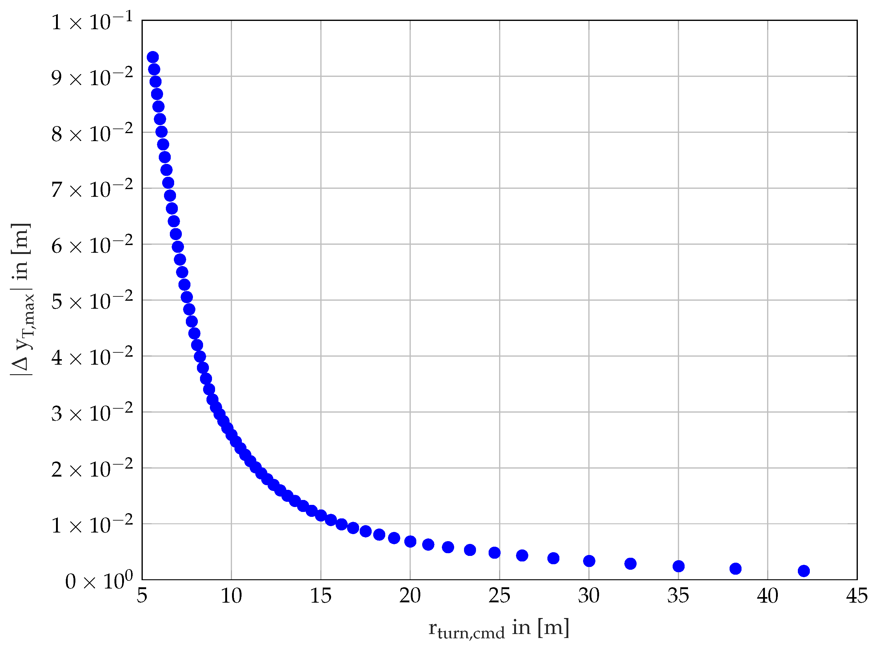
4.2. Turn Radius Influence on Maximal Error

This example deals with an analysis of the turn radius influence on the maximal lateral deviation allowed by the controller. Therefore, a ${180}^{\circ }$ turn is considered, while the aircraft velocity is set to $V_K=22\mathrm{m}/\mathrm{s}$, which corresponds to a typical flight velocity of a small unmanned aerial vehicle. Initially, the aircraft’s position and the desired trajectory match.

First, Figure 2 shows the maximum lateral deviation of the ${180}^{\circ }$-turn for different turn radii. It is clear that for a smaller turn radius, i.e., a tighter, more aggressive maneuver, the lateral deviation error is increased. Still, the maximum error is only around $0.1\mathrm{m}$ at a turn radius of approximately $5\mathrm{m}$, which shows the capabilities of the proposed controller for highly accurate trajectory control. It is furthermore seen that for gentle maneuvers, i.e., an increased turn radius, the lateral deviation asymptotically approaches zero. The remaining magnitude of the error is hereby mainly related to the model lags introduced in Equation (12). It should be further noted that it is expected that the maximum lateral deviation decreases further when not only the specific force is commanded to the aircraft but also its derivative. Then, the reaction to deviations is improved even further and the introduced lags in Equation (12) can be directly accounted for.

Continuing, Figure 3 displays the maximum absolute lateral specific force along the ${180}^{\circ }$-turn. As expected, a higher lateral force is required to follow a tighter, i.e., more aggressive, turn maneuver. This strengthens the argumentation used before in Figure 2 that a more aggressive maneuver, yielding a larger lateral specific force requirement, results in a greater deviation. Still, as also already seen in Figure 2, even a considerable lateral specific force of around $9\mathrm{m}/{\mathrm{s}}^2$ only yields to a tolerable lateral deviation of $0.1\mathrm{m}$.

Concluding, this application example shows the applicability of the proposed trajectory controller in scenarios with high accuracy demand. Specifically, both gentle as well as aggressive maneuvers are handled by the proposed scheme.

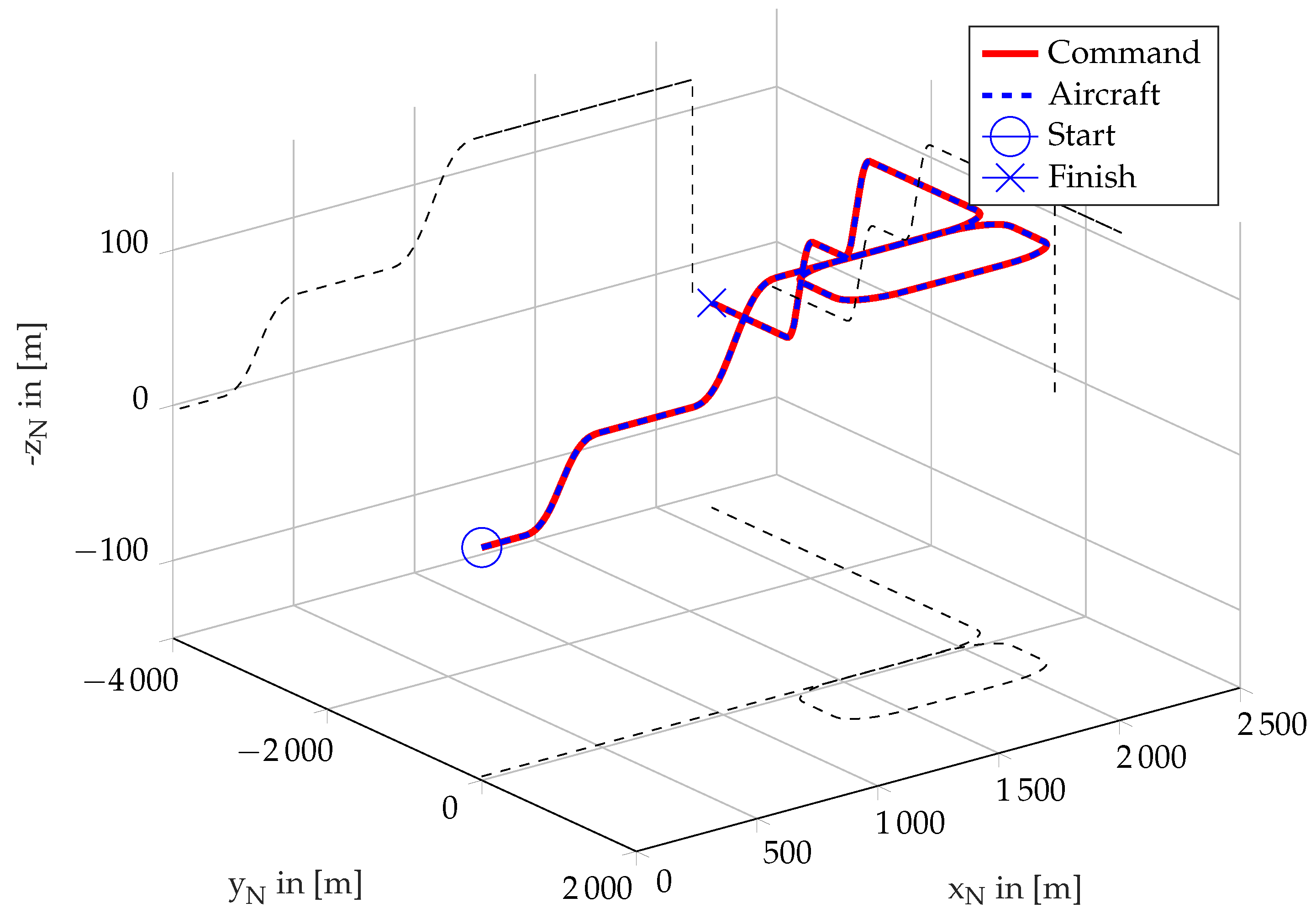
4.3. Four-Dimensional Trajectory Control

The application section concludes with an example of a complex trajectory following task. Here, Figure 4 shows the desired/commanded (solid red) vs. the actually flown (dashed blue) trajectory for a complex climb and turn maneuver including a holding. Furthermore, the planar projections (dashed black) of the maneuver are shown for convenience and to get a better overview of the maneuver structure.

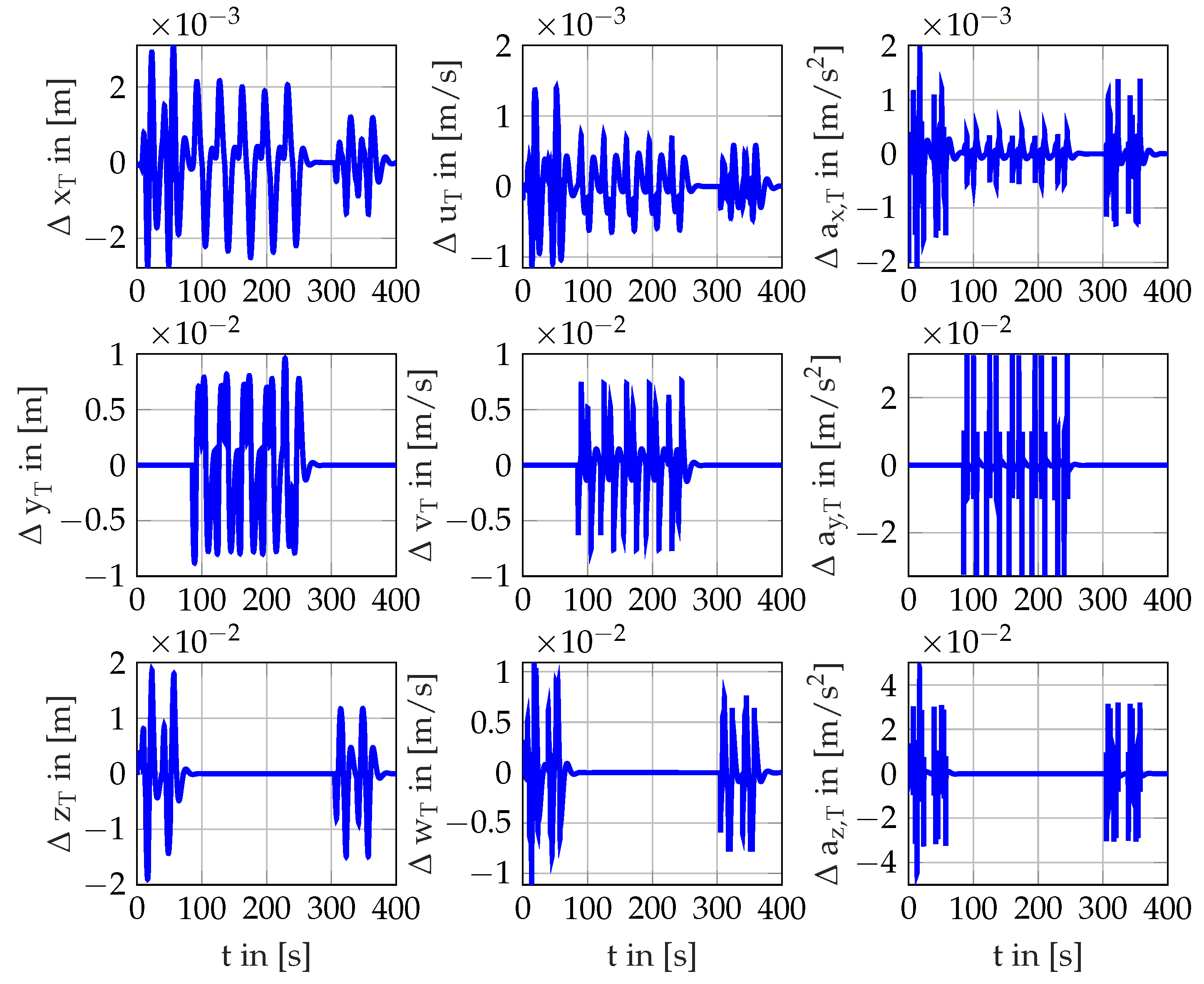
Then, Figure 5 shows the position, velocity, and acceleration deviations obtained from following the trajectory in Figure 4. It can be seen that maximum vertical errors of $\pm 0.02\mathrm{m}$ occur in climb/descent segments, while the maximum lateral deviation is around $\pm 0.01\mathrm{m}$. In general, the horizontal deviation shows the overall best tracking.

This overall shows the high accuracy of the controller. Additionally, the errors are rapidly reduced, which is specifically obtained due to the error controller that already starts acting at the acceleration deviation level. In this context, it can be seen that maximum vertical acceleration deviation of $\pm 0.05\mathrm{m}/{\mathrm{s}}^2$ and of $\pm 0.01\mathrm{m}/\mathrm{s}$ for velocity is achieved. This shows both the fast response of the controller to deviations as well as the smoothness, i.e., that small deviations are controlled with small control effort.

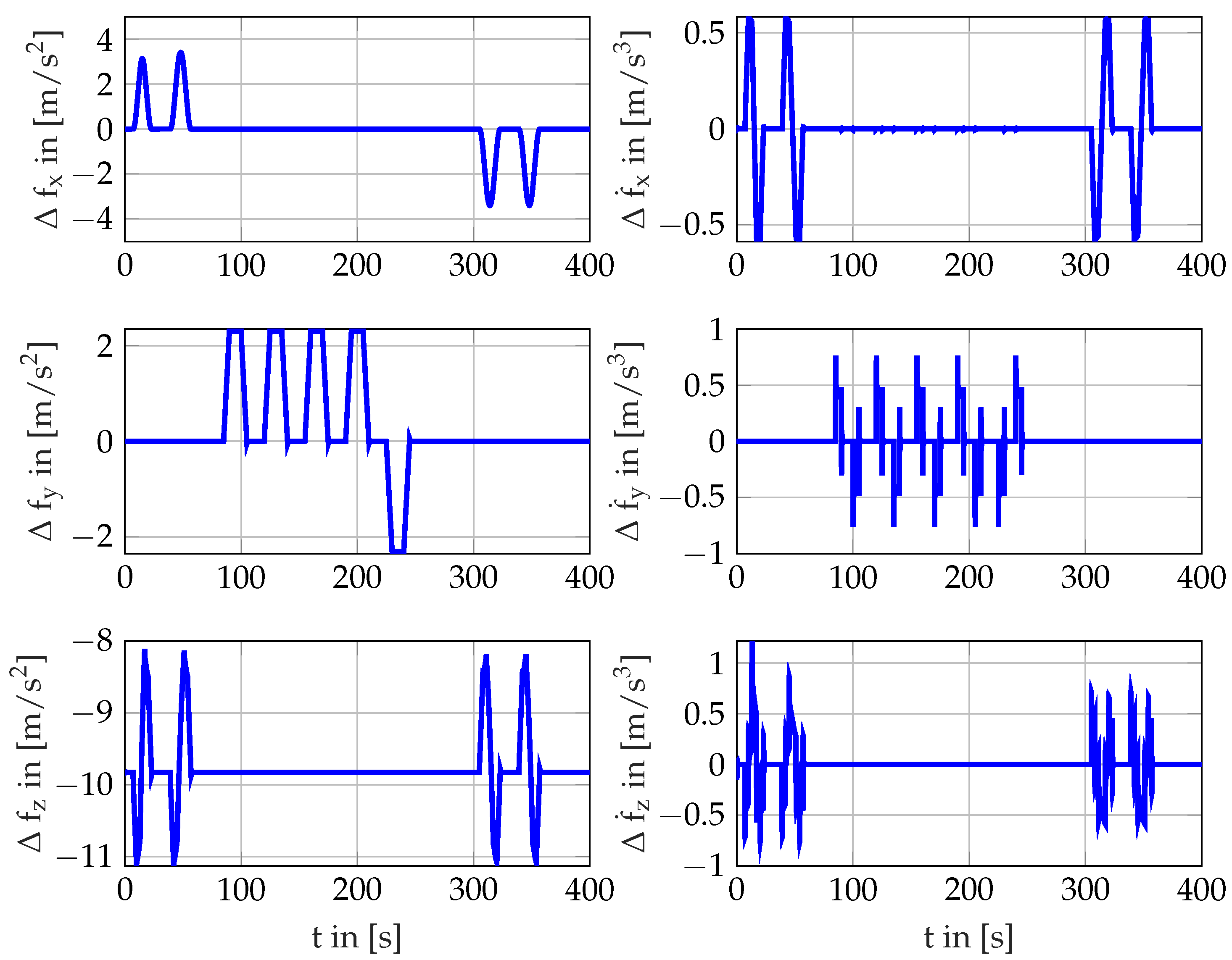
Finally, Figure 6 shows the specific forces and their derivatives commanded to the model when following the trajectory in Figure 4. It is specifically seen that a high smoothness for the specific forces as well as the decoupling of the axes by nonlinear dynamic inversion is achieved, which results in a more physical command for controlling the aircraft. Still, it is clearly seen that the specific force derivatives directly react to the deviations in Figure 5. Specifically, it can be observed that the specific force derivatives counteract the acceleration errors in Figure 5. Furthermore, it is seen that there are generally no high-frequency oscillations in the command signal, which is a specific consequence of the fact that the nonlinear aircraft kinematics are considered by the controller. Due to these, it is known how the aircraft can move, and thus the controller does not try to compensate deviations by large control effort but by reasonable magnitudes and dynamics that the aircraft is able to follow.

5. Conclusions

A novel trajectory controller utilizing full nonlinear kinematics on the jerk-level between the reference point of the dynamic model and the planned trajectory foot point was developed in this study. The resulting nonlinear error dynamics was controlled using a nonlinear dynamic inversion control law that connected jerk-based nonlinear error dynamics with kinematic equations of motion. The proposed scheme was applied in an aircraft-related context and shows promising results and significant capabilities in controlling the trajectory/path with a high accuracy.

Further work naturally starts with an incorporation of the trajectory controller into a real flying vehicle to show the capabilities in real flight test. Additionally, surveys on choosing suitable commands other than zero for the desired jerk command should be conducted to achieve, e.g., optimal minimum jerk trajectories. Finally, the gain tuning within the pseudocontrol in Equation (11) should be addressed. To this end, it is especially interesting to consider the nature of the derived nonlinear error dynamics in Equation (9), which are of a linear, parameter-varying type. Here, sophisticated analysis methods can be used to significantly boost performance and already ensure stability as well as desired behavior of the error dynamics in connection with a suitable design of the reference trajectory.