Impact of Horse Hoof Wall with Different Solid Surfaces

Abstract

This study aimed to investigate the impact of a horse hoof wall on three solid surfaces: steel, concrete and asphalt. Impact experiments were conducted for different impact angles and different initial impact velocities. The effect of impact surfaces, impact angles and initial impact velocities on the coefficient of restitution and the effective coefficient of friction were tested using one-way ANOVA. Analytical and numerical modeling of the impact were developed. The impact interval was divided into two phases: compression and restitution. For compression, a contact force with a damping term was used. The restitution was characterized by an elastic contact force. The stiffness and damping coefficients of the contact force were estimated from the normal impacts. The simulated velocities after the oblique impacts were compared to the velocities in the in vitro investigation. The coefficient of restitution varied significantly on different surfaces. The effective coefficient of friction was lower on steel compared to concrete and asphalt. The model presented in this study can be applied to refine the impact simulation of the equine hoof during locomotion.

1. Introduction

Impact is considered the most critical phase of the gait cycle for developing musculoskeletal injuries [1,2,3]. The hoof wall is the weight-bearing and protecting structure surrounding the distal phalanx of the horse. During impact, the hoof wall repetitively withstands concussive forces and transmits the forces to the bones and joints of the limb. During impact, the hoof wall must resist excessive abrasion in order to protect interior structures [4]. The reaction forces on the hoof during impact involve two dynamic processes. Low impact loads at high vibration frequency characterize the collision of the hoof with the ground, followed by high forces at low frequency which are largely attributable to the onset of the collision of the torso with the limb [5,6,7]. Factors that affect initial impact vibrations are the specialized tissues of the hoof wall, the ground surface and the shoe if the horse is shod.

Equine hoof wall is an anisotropic composite material composed of keratin; it appears to be one of the most fracture-resistant biological structures known [8]. Investigation of the surface strains of the hoof wall under different locomotion conditions indicate that the wall is loaded principally in compression [9,10]. Mechanical tests of the equine hoof wall indicate that the wall is stiffer in compression than in tension [11]. The effect of hoof wall viscoelasticity on the mechanical properties have been evaluated with the results suggesting that the stiffness increased with stain rate, while the fracture resistance was unaffected by strain rate [12]. The fracture resistance of the equine hoof wall is correlated with the morphological organization of the keratin tissue [13]. The level of hydration of the hoof wall normally decreases from interior to outer surfaces and from the proximal region to the distal margin. The effect of hydration on the material properties of hoof keratin has been investigated and it was found that stiffness decreased with moisture content whereas maximal fracture toughness was reached at a state of intermediate hydration [14]. Knowing the material properties of the equine hoof components, hoof capsule mechanics have been explored using finite element methods [15,16].

The shock and vibration at initial impact are absorbed and attenuated by the ground surface. Hoof acceleration and ground reaction forces of horses trotted on different surfaces revealed that the ground surface has a great effect on the maximum deceleration and impact forces [17,18,19]. Therefore composition of the ground surface is likely to affect the potential for injury by altering the force transmitted from the ground to the hoof and the propagation of the forces to limb structures [20]. Sliding of the hoof on the ground is considered to be a cause of soft-tissue injury and occurs when the horizontal deceleration force exceeds the maximal friction [21,22]. The coefficients of friction between cadaver horse hooves and different solid substrates and racetrack soil have been investigated with the results suggesting that the hoof has good traction on most rough surfaces [21,22,23].

Application of a shoe to the hoof wall has the potential to alter the interaction between the hoof and the ground, and therefore, has an effect on the risk of musculoskeletal injuries [1]. Evaluation of the impact forces under different shoeing conditions suggested that synthetic shoes attenuate hoof impact at a trot [3,24], while a finite element analysis showed that the steel shoe might increase the mechanical loading on the bones of the distal limb [25].

Contact force models have been extensively explored in studies of human locomotion. A typical model consisting of parallel linear spring-damper elements, also referred to as the Kelvin–Voigt model [26], has been applied to simulate the ground reaction force during human running [27,28]. Hunt and Crossley [29] proposed a nonlinear contact model using Hertz theory with a hysteresis damping which has been applied in simulating foot-ground interaction of a walking machine [30]. Liu and Nigg proposed a nonlinear model with combined material properties of heel pad, shoe and ground [31]. Ly et al. modified Liu and Nigg’s model to explicitly distinguish the ground reaction force with the force between the foot and the shoe [32]. In their model, the ground-shoe interaction was characterized by a linear function of the ground stiffness and the force between the foot and the shoe sole was modeled by the Hertz contact law with a linear damping.

Rigid body dynamics were also used to simulate the stance phase of horse locomotion. Linear spring damper models have been considered in simulating the horizontal and vertical interaction of the hoof with the ground [5]. A linear viscoelastic model and a pseudo-Coulomb friction model have been adopted to approximate the ground reaction forces in vertical and horizontal directions, respectively, where the parameters were chosen to produce practical ground penetration and sliding speed [33]. A nonlinear spring damper model was used to simulate the vertical loading of the equine limb galloping on the racetrack where the stiffness and damping properties of the hoof were estimated based on the data derived from other animals [34]. It has been shown that the racetrack surface stiffness properties have a greater effect on loading than the surface damping properties. Liu and Nigg’s nonlinear contact model [32] was applied to simulate the reaction force between the shoe and the ground at gallop [35].

We proposed a new contact force for the impact of the hoof with different surfaces. This contact force is viscoelastic for the compression and elastic for the restitution. This type of force was not used in previous studies and is validated by experiments. The purpose of this study was to provide quantitative comparison of the interaction of horse hoof with different surfaces and present a numerical model based on two phases of impact (compression and restitution). For each phase of impact, contact forces were developed. The impact surfaces were steel, concrete and asphalt. Steel is the most common material used for modern horseshoes. Equine lameness examinations are often conducted on a concrete or an asphalt surface.

2. Materials and Methods

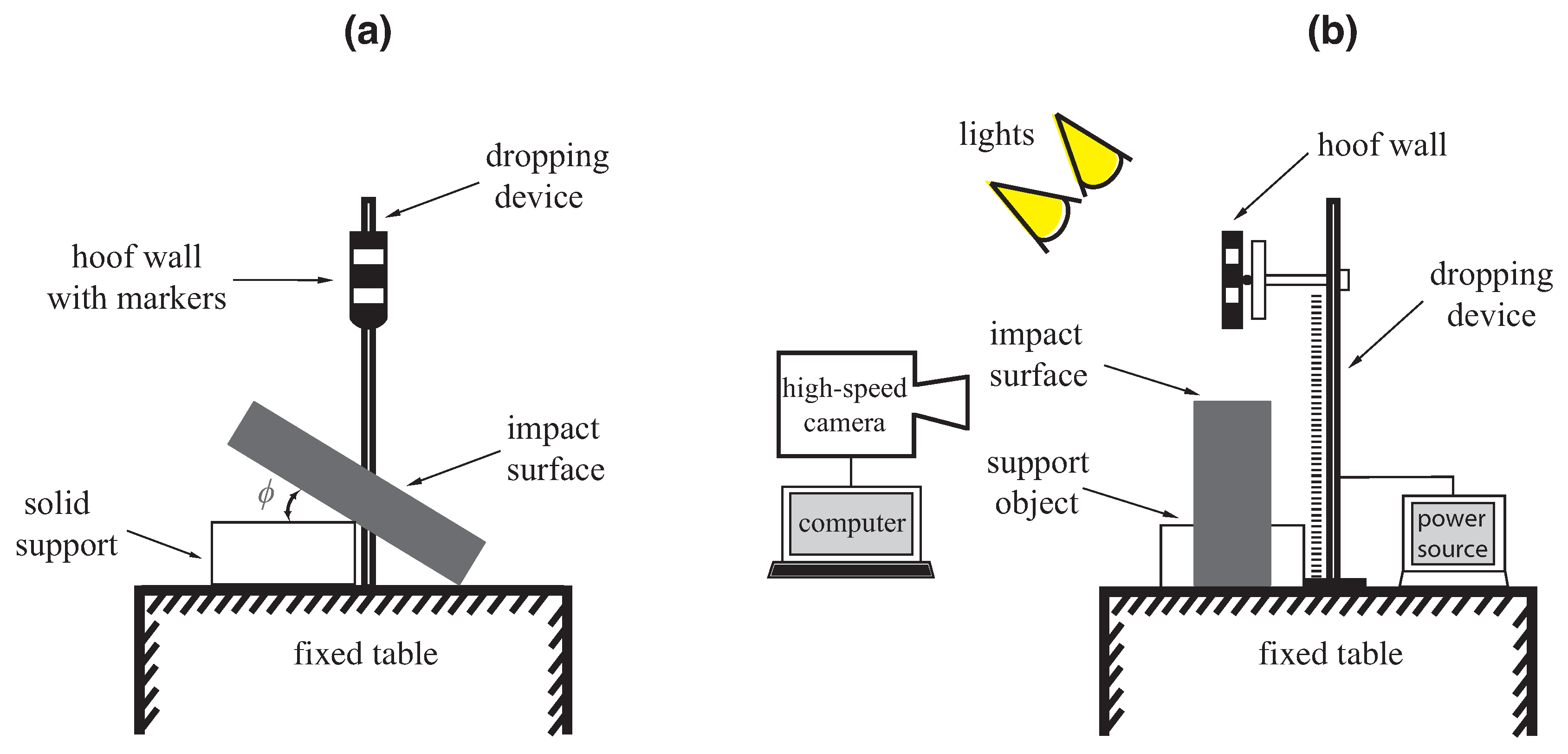
2.1. Experiments

The dorsal hoof wall specimen used in this study was obtained from the forelimb of a female Percheron cadaver. The wall was cut into a $0.045$ m long by $0.016$ m wide by $0.008$ m high section. One end of the longitudinal dimension was machined into round with a radius $R=0.009$ m. The mass of the wall specimen was $m=0.008$ kg.

The experimental setup, shown in Figure 1, was built for the impact of the hoof wall with different surfaces. The hoof wall was held in its initial position and released by a dropping device. The dropping position could be adjusted to provide different initial impact velocities for the hoof wall. The angle of the impact surface $\varphi$ was adjusted with a solid support placed under the impact surface. The support and the impact surface were fixed during the experiment. The steel, concrete and asphalt were used as the impact surface. Different initial impact velocities within 1.5–4 m/s were selected to approximate the magnitude of hoof landing velocity in trotting horses [36,37]. Four impact angles $0,{10}^{\circ },{20}^{\circ }\mathrm{and}{30}^{\circ }$ were tested. Three tests were performed for each combination of surface, impact angle and initial impact velocity.

Black and white markers were attached to the hoof wall as shown in Figure 1. A high-speed camera (NAC Hot Shot SC, NAC Image Technology Inc., Tokyo, Japan) with 8000 frames per second was used to track the motion of the white markers on the wall before and after impact. Triggering of the camera and release of hoof wall were simultaneous. Two 1000 W lights were used to provide sufficient visual separation for the camera. For each experiment, 20 frames before impact and 20 frames after impact were used to estimate the linear and angular velocities of the hoof wall. A high-speed camera provides appropriate accuracy in capturing kinematic data [38,39] The image processing was performed in MATLAB (Matlab R2018b, MathWorks Inc., Natick, MA, USA).

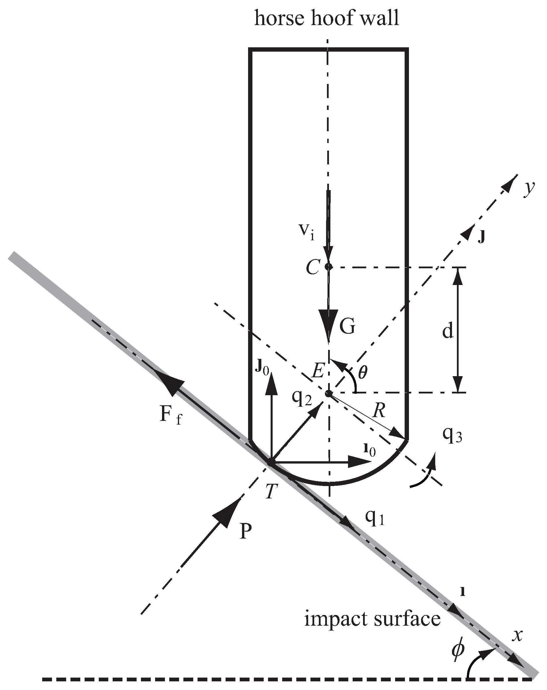
2.2. Mathematical Modeling

Figure 2 shows the schematic of the hoof wall during the impact with a solid surface. The angle of the impact surface with the horizontal axis is $\varphi$. The contact point on the hoof wall is T. The distance between the center of mass C and center of the circular end E of the hoof wall is d. The radius of the circular end is R. The unit vectors ${\mathit{ı}}_0$, ${\mathit{j}}_0$ and ${\mathit{k}}_0$ with the origin at the contact point T form a global reference frame. Let ı, j and $\mathit{k}$ be the unit vectors that form a local reference frame at the same origin with x-axis along the impact surface. To characterize the configuration of the hoof wall, the generalized coordinates $q_1,q_2,q_3$ were selected. Coordinates $q_1,q_2,q_3$ denote the displacement of the contact point T along $x,y,z$ directions, respectively. Forces acting on the hoof wall during impact are gravity $\mathbf{G}$, normal contact force $\mathbf{P}$ and friction force ${\mathbf{F}}_f$.

The position of the contact point T was ${\mathbf{r}}_T=q_1\mathit{ı}+q_2\mathit{j}$. The position of the center of the circular end E was ${\mathbf{r}}_E=q_1\mathit{ı}+(q_2+R)\mathit{j}$. The position of the center of mass C was calculated by ${\mathbf{r}}_C=(q_1+dcos{q}_3)\mathit{ı}+(q_2+R+dsin{q}_3)\mathit{j}$. The angular velocity and acceleration of the hoof wall were $\mathit{\omega }={\dot{q}}_3\mathit{k}\mathrm{and}\mathit{\alpha }={\ddot{\mathrm{q}}}_3\mathit{k}$. The velocity and acceleration of the center of the circular end E were ${\mathbf{v}}_E=\frac{d{\mathbf{r}}_E}{dt}\mathrm{and}{\mathbf{a}}_{\mathrm{E}}=\frac{{\mathrm{d}}^2{\mathbf{r}}_{\mathrm{E}}}{{\mathrm{dt}}^2}$. The velocity and acceleration of the contact point T were ${\mathbf{v}}_T={\mathbf{v}}_E+\mathit{\omega }\times ({\mathbf{r}}_T-{\mathbf{r}}_E)\mathrm{and}{\mathbf{a}}_{\mathrm{T}}={\mathbf{a}}_{\mathrm{E}}+\mathit{\alpha }\times ({\mathbf{r}}_{\mathrm{T}}-{\mathbf{r}}_{\mathrm{E}})+\mathit{\omega }\times \left[\mathit{\omega }\times ({\mathbf{r}}_{\mathrm{T}}-{\mathbf{r}}_{\mathrm{E}})\right]$. The velocity and acceleration of the center of mass C were ${\mathbf{v}}_C={\mathbf{v}}_E+\mathit{\omega }\times ({\mathbf{r}}_C-{\mathbf{r}}_E)\mathrm{and}{\mathbf{a}}_{\mathrm{C}}={\mathbf{a}}_{\mathrm{E}}+\mathit{\omega }\times ({\mathbf{r}}_{\mathrm{C}}-{\mathbf{r}}_{\mathrm{E}})+\mathit{\omega }\times \left[\mathit{\omega }\times ({\mathbf{r}}_{\mathrm{C}}-{\mathbf{r}}_{\mathrm{E}})\right]$.

Gravitational force was calculated as $\mathbf{G}=mgsin\varphi \mathit{ı}-mgcos\varphi \mathit{j}$, where m is the mass of the hoof wall and $g=9.81\mathrm{m}/{\mathrm{s}}^2$ is the gravitational acceleration. The normal contact force acting on the contact point T was along y-axis with an expression $\mathbf{P}=P\mathit{j}$. The friction force was calculated by ${\mathbf{F}}_f=-\mu \left|P\right|\frac{{\mathbf{v}}_T·\mathit{ı}}{|{\mathbf{v}}_T·\mathit{ı}|}\mathit{ı}$, where $\mu$ is the kinetic coefficient of friction. Newton–Euler equations of motion were developed for the impact analysis: $m{\mathbf{a}}_C=\mathbf{G}+\mathbf{P}+{\mathbf{F}}_f\mathrm{and}{\mathrm{I}}_{\mathrm{C}}\mathit{\alpha }=({\mathbf{r}}_{\mathrm{T}}-{\mathbf{r}}_{\mathrm{C}})\times (\mathbf{P}+{\mathbf{F}}_{\mathrm{f}})$, where $I_C$ is the mass moment of inertia about the center of mass C.

The impact was divided into two phases: compression and restitution. The compression phase started when the hoof wall contacted the impact surface with the initial impact velocity $v_i$ and continued until the maximum compression, ${\delta }_m$, was reached. At the maximum compression, the normal velocity of the contact point T became zero, i.e., ${\mathbf{v}}_T·\mathit{j}=0$. Next, the restitution phase began and ended when there was no contact between the hoof wall and the impact surface.

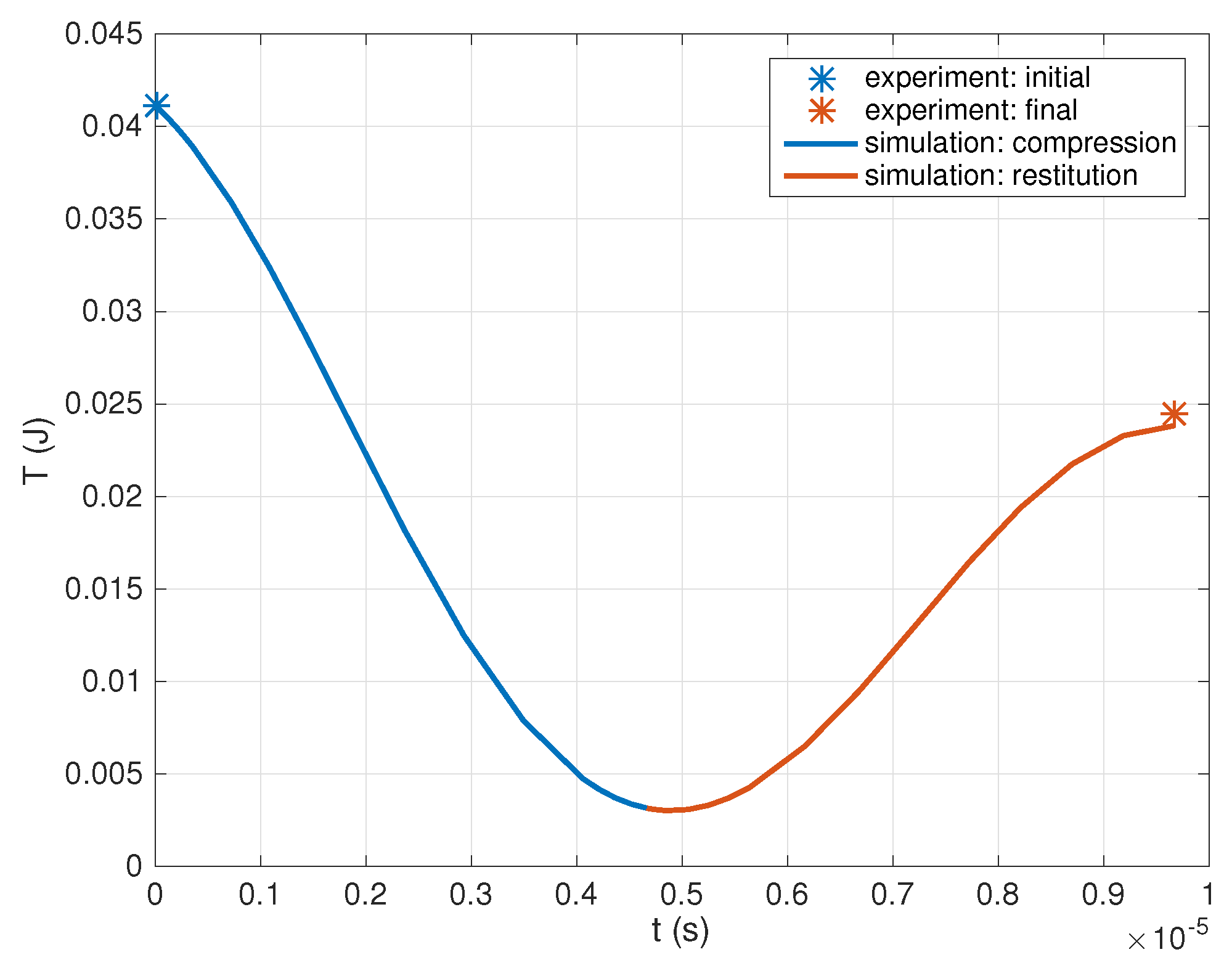
2.2.1. Compression Phase

The spring damper model was used for the normal contact force during the compression phase [26,27],

$$P=-k\delta -b\dot{\delta },$$

(1)

where k is the stiffness coefficient and b is the damping coefficient, $\delta =q_2$ is the normal elastic displacement of the impact surface. At the beginning of the compression phase, $\delta =0$. The initial conditions for compression phase were $q_1\left(t_i\right)=q_{1i},{\dot{q}}_1\left(t_i\right)=v_{i}sin\varphi ,q_2\left(t_i\right)=q_{2i},{\dot{q}}_2\left(t_i\right)=-v_{i}cos\varphi ,q_3\left(t_i\right)=\varphi +{90}^{\circ },{\dot{q}}_3\left(t_i\right)=0$, where $v_i$ is the velocity of the hoof wall when it first contacted the impact surface and $v_i$ was obtained from the experiment, $\varphi$ is the angle of the impact surface with the horizontal axis. Since the hoof wall is in contact with the impact surface at this moment, $q_{1i}=q_{2i}=0$.

2.2.2. Restitution Phase

The restitution phase started at the moment of maximum compression. During this phase, the contact force decreased from the maximum value to zero. It was assumed that the restitution is fully elastic as it has been proved in contact mechanics area [40,41,42]. The normal contact force was given by

$$P=-k\delta .$$

(2)

At the end of the restitution phase $\delta =0$ and $P=0$. The initial conditions for restitution phase were the conditions at maximum compression: $q_1\left(t_m\right)=q_{1m},{\dot{q}}_1\left(t_m\right)={\mathbf{v}}_E\left(t_m\right)·\mathit{ı},q_2\left(t_m\right)={\delta }_m,{\dot{q}}_2\left(t_m\right)=0,q_3\left(t_m\right)=q_{3m},{\dot{q}}_3\left(t_m\right)={\omega }_m$. The nonlinear differential equations of motion with initial conditions were solved in MATLAB using ODE45 function.

To model the process of energy transfer in impact, the coefficient of restitution and effective coefficient of friction were employed [43],

$$e=\left|\frac{{\mathbf{v}}_T\left(t_f\right)·\mathit{j}}{{\mathbf{v}}_T\left(t_i\right)·\mathit{j}}\right|,$$

$$\mu =\left|\frac{{\mathbf{v}}_C\left(t_f\right)·\mathit{ı}-{\mathbf{v}}_C\left(t_i\right)·\mathit{ı}}{{\mathbf{v}}_C\left(t_f\right)·\mathit{j}-{\mathbf{v}}_C\left(t_i\right)·\mathit{j}}\right|,$$

where ${\mathbf{v}}_C\left(t_f\right)$ and ${\mathbf{v}}_T\left(t_f\right)$ are the velocity of the center of mass C and contact point T at the end of the restitution phase. The coefficient of restitution and effective coefficient of friction were estimated from the experiments.

The stiffness coefficient k and damping coefficient b were determined by an optimizing procedure which altered k and b to find the best fit between the experimental and the simulated velocity after normal impact. The coefficient k was varied between $k=1\left({10}^5\right)\mathrm{and}1\left({10}^9\right)$ N/m and the coefficient b was varied between $0\mathrm{and}2000$ N s/m. Mean percentage error between the experimental and the simulated velocity after impact was calculated. Optimal model coefficient combinations were determined by minimizing the mean percentage error. The coefficients were estimated from normal impact because oblique impact was affect by friction which could bring additional experimental error into the estimation process. On the other hand, the experimental result from normal impact was considered to be more accurate since out-of-plane rotation of the hoof wall was less likely to occur in this case.

The estimated coefficients were then used to predict the velocity after oblique impact. Furthermore, the predicted velocity was compared with the experimental result to verify the model. In some cases where the permanent deformation is significant, the indentation after impact can be measured by an optical profilometer to verify the model [38]. In other cases where the impact bodies are metallic, the duration of impact can be recorded by a digital oscilloscope to validate the model [44]. However, neither of these two methods were applicable to this study.

2.3. Statistical Analysis

One-way analyses of variance (ANOVA) were used to determine whether there were significant differences in the coefficient of restitution and effective coefficient of friction, among the different impact surfaces, impact angles and initial impact velocities, respectively. The equality of variances were investigated using Bartlett’s test. Variance-stabilizing transformations were performed when the homogeneity of variances were violated. If a significant difference was found, a multiple comparison using the least significant difference (LSD) procedure was conducted to further explore which pairs of means were different and which pairs of means were not. Statistical analyses were carried out using a statistical software (SAS Studio 3.8, SAS Institute Inc., Cary, NC, USA). Significant level was set at $p<0.05$.

3. Results

Figure 3 shows the displacement of the hoof wall before and after impact on steel with the initial impact velocity $v_i=3.28$ m/s and the impact angle $\varphi ={20}^{\circ }$. The hoof wall impacts the surface vertically and then rebounds counterclockwise. The displacement of the center of mass ${\mathbf{r}}_C$ in local coordinates $q_1,q_2,q_3$ is plotted in Figure 3a and the angular position $\theta$ of the hoof wall with the horizontal axis is depicted in Figure 3b. The impact occurred at $t=0.0025$ s. The angle $\theta$ maintained at ${90}^{\circ }$ before impact and increased continuously after impact. The velocity of the center of mass before impact was calculated as ${\mathbf{v}}_C\left(t_i\right)=1.18\mathit{ı}-3.05\mathit{j}$ m/s. The velocity of the center of mass after impact was calculated as ${\mathbf{v}}_C\left(t_f\right)=0.51\mathit{ı}+2.26\mathit{j}$ m/s.

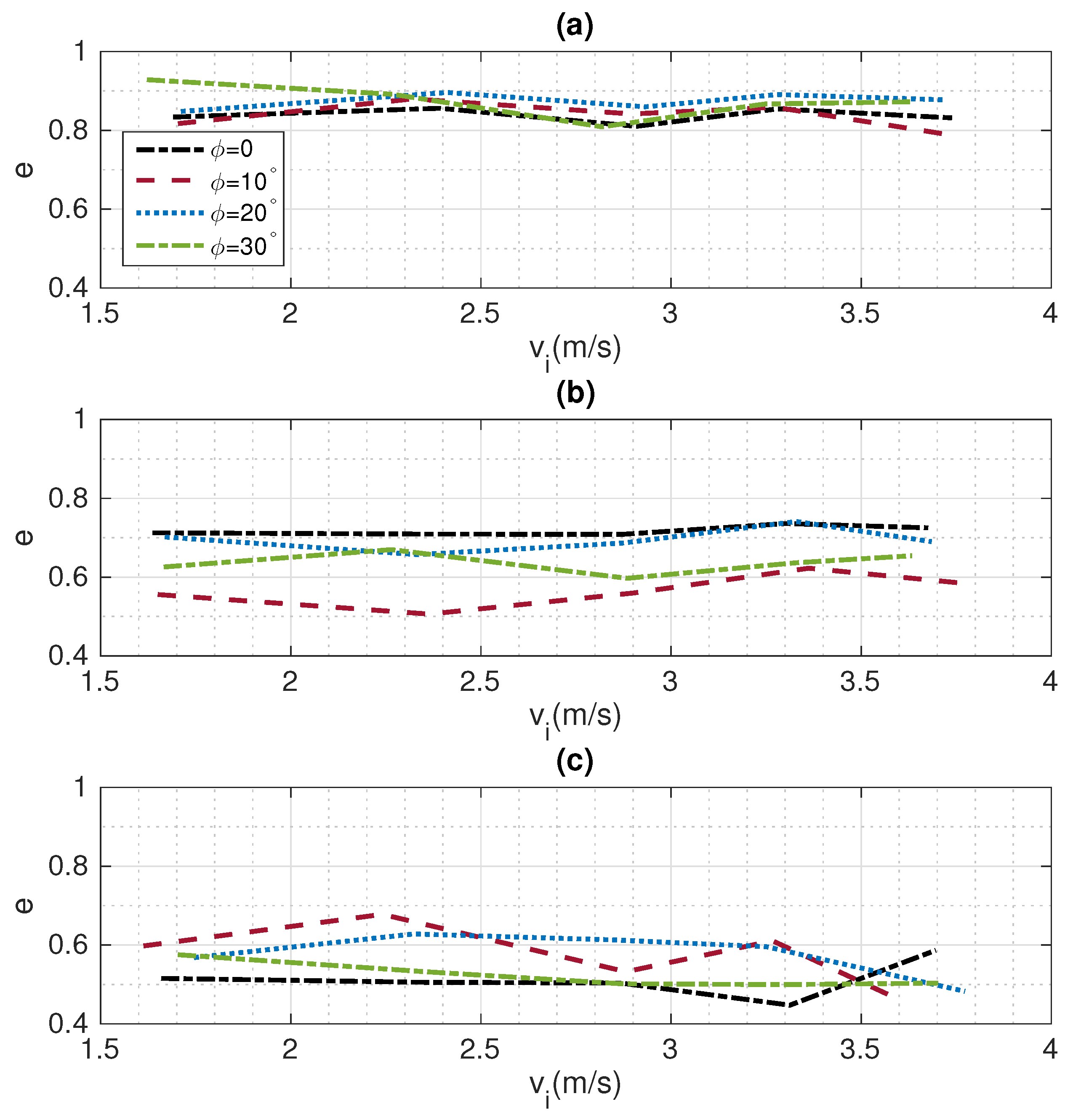
3.1. Coefficient of Restitution

Figure 4 shows the mean coefficients of restitution for different impact surfaces at various impact angles and initial impact velocities. The mean coefficients of restitution for steel were 0.84 (s.d. 0.041), 0.84 (s.d. 0.042), 0.87 (s.d. 0.049), 0.88 (s.d. 0.070) for $\varphi =0,{10}^{\circ },{20}^{\circ },{30}^{\circ }$, respectively, where s.d. is the standard deviation. The mean coefficients of restitution for concrete were 0.72 (s.d. 0.039), 0.57 (s.d. 0.050), 0.70 (s.d. 0.043), 0.64 (s.d. 0.076) for $\varphi =0,{10}^{\circ },{20}^{\circ },{30}^{\circ }$, respectively. The mean coefficients of restitution for asphalt were 0.51 (s.d. 0.071), 0.57 (s.d. 0.079), 0.58 (s.d. 0.071), 0.52 (s.d. 0.086) for $\varphi =0,{10}^{\circ },{20}^{\circ },{30}^{\circ }$, respectively. Significantly higher coefficients of restitution were seen on steel compared with concrete ($p<0.0001$) and asphalt ($p<0.0001$). Coefficients of restitution on concrete were significantly higher than coefficients of restitution on asphalt ($p<0.0001$). However, coefficients of restitution did not show any significant differences among various impact angles ($p=0.1603$) and initial impact velocities ($p=0.9476$).

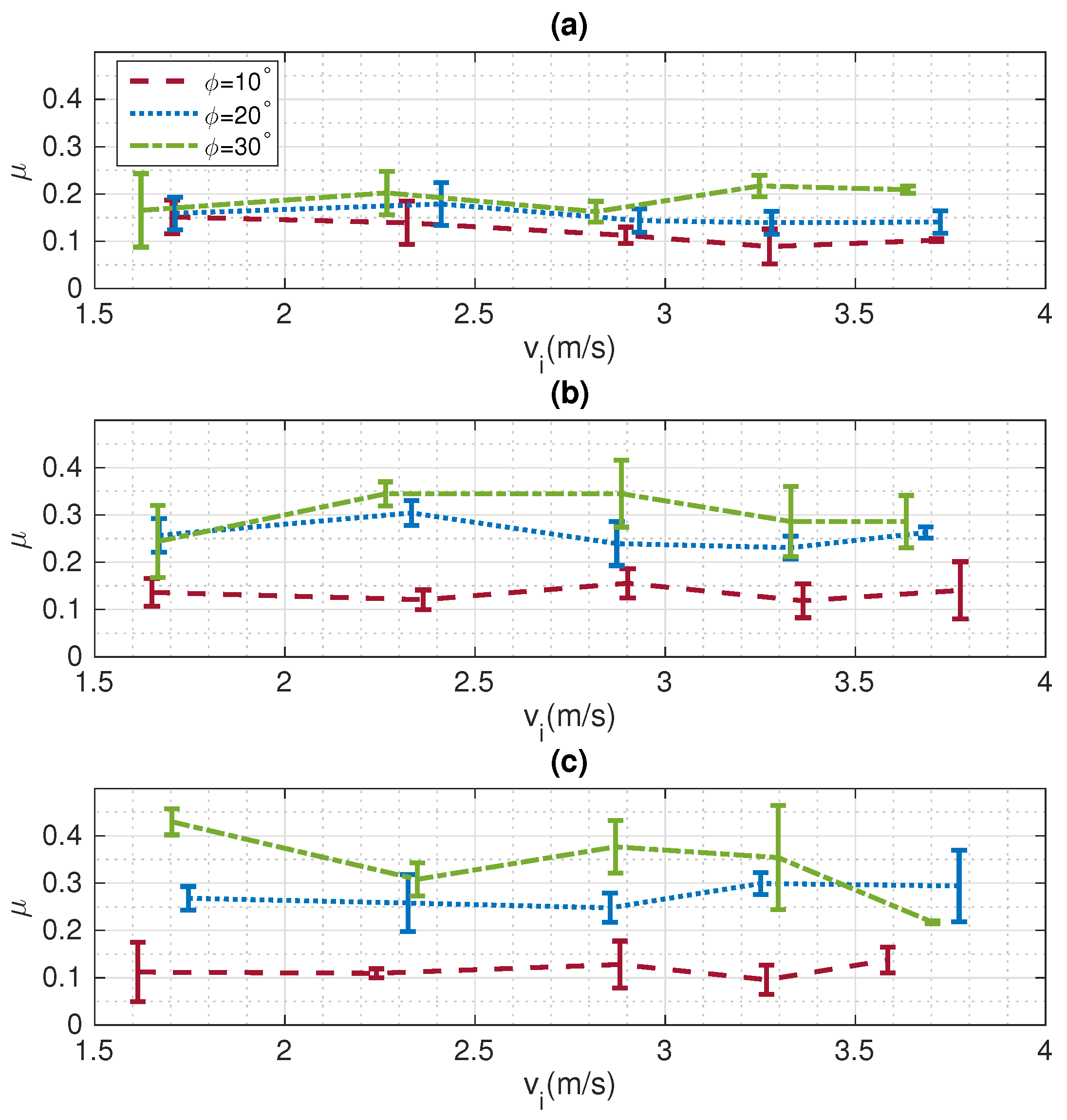
3.2. Effective Coefficient of Friction

Figure 5 shows the mean effective coefficients of friction for different impact surfaces at various impact angles and initial impact velocities. The mean effective coefficients of friction for steel were 0.12 (s.d. 0.036), 0.15 (s.d. 0.030), 0.19 (s.d. 0.044) for $\varphi ={10}^{\circ },{20}^{\circ },{30}^{\circ }$, respectively. The mean effective coefficients of friction for concrete were 0.13 (s.d. 0.035), 0.26 (s.d. 0.037), 0.30 (s.d. 0.062) for $\varphi ={10}^{\circ },{20}^{\circ },{30}^{\circ }$, respectively. The mean effective coefficients of friction for asphalt were 0.12 (s.d. 0.039), 0.27 (s.d. 0.042), 0.34 (s.d. 0.089) for $\varphi ={10}^{\circ },{20}^{\circ },{30}^{\circ }$, respectively. Significantly lower effective coefficients of friction were seen on steel compared with concrete ($p=0.0007$) and asphalt ($p=0.0002$). Effective coefficients of friction on concrete and asphalt were not significantly different ($p=0.7271$). Significantly higher effective coefficients of friction were found at larger impact angles ($p<0.001$). Effective coefficients of friction did not show any significant differences among various initial impact velocities ($p=0.8421$).

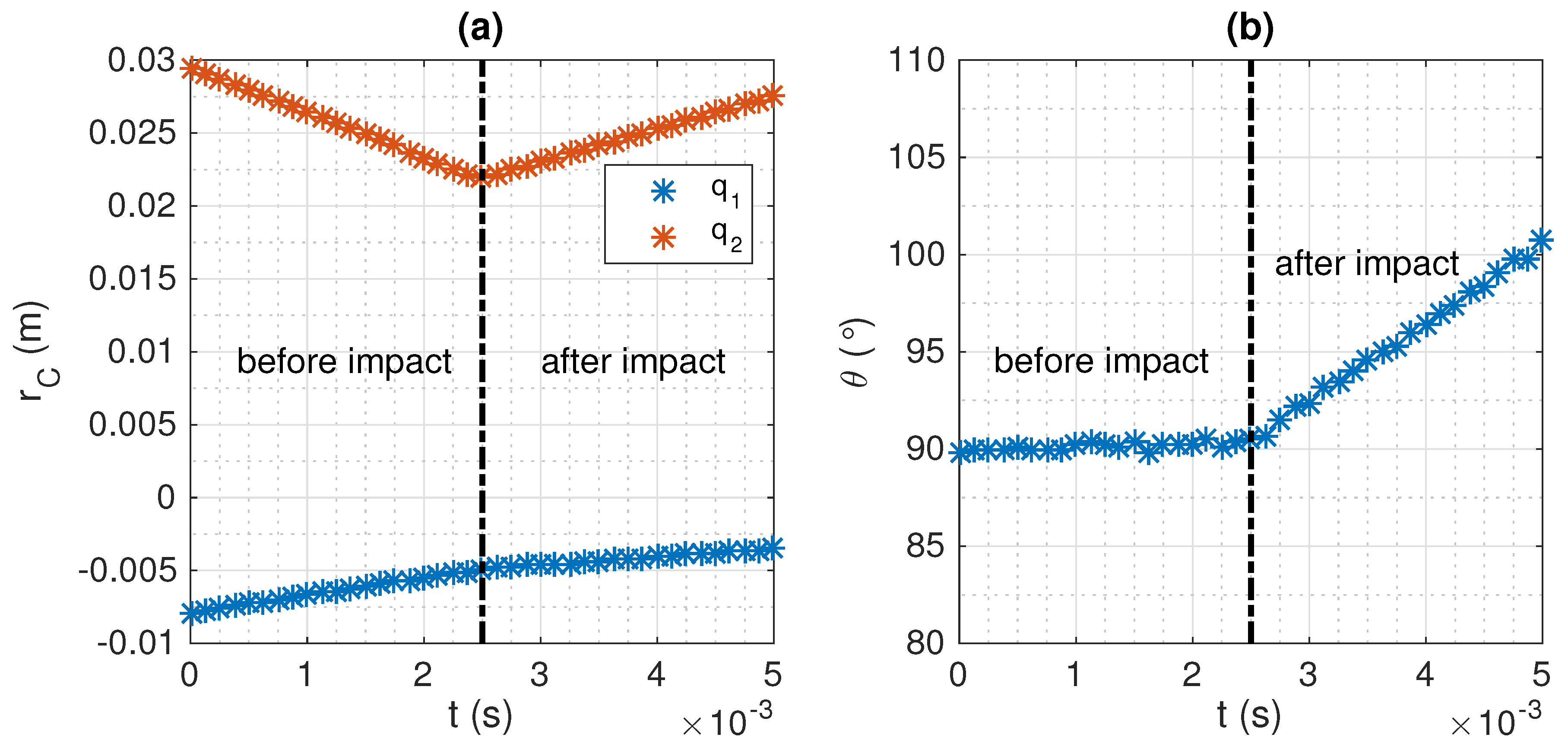
3.3. Normal Impacts and Contact Force Coefficients

Figure 6 shows the mean experimental and simulated velocities of the center of mass after normal impact on different surfaces. The mathematical model was able to fit the experimental velocities with good accuracy across initial impact velocities. The stiffness coefficients used in Figure 6 were $k=7.24\left({10}^8\right),4.24\left({10}^8\right),\mathrm{and}5.86\left({10}^7\right)$ N/m for steel, concrete and asphalt, respectively. The damping coefficients used in Figure 6 were $b=531.65,932.20,\mathrm{and}822.78$ N s/m for steel, concrete and asphalt, respectively.

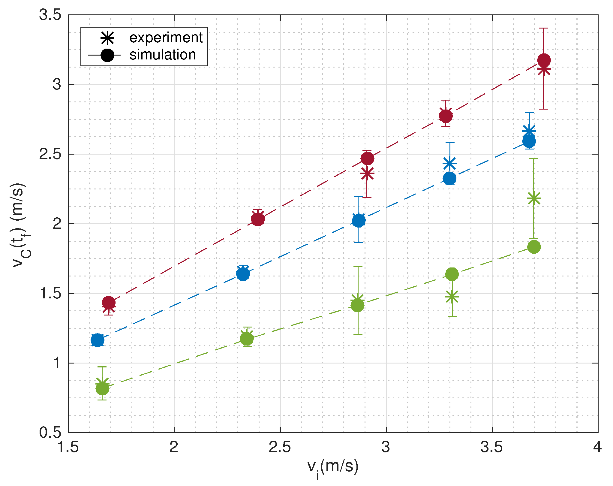
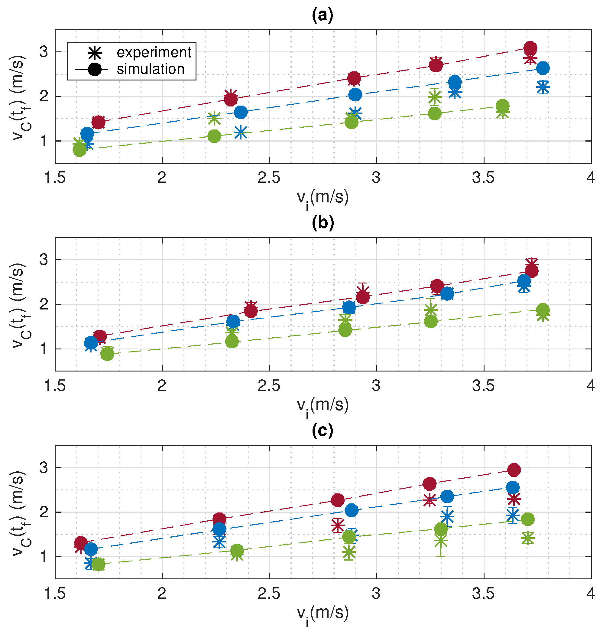
3.4. Oblique Impacts

The velocities of the center of mass after oblique impacts were simulated using the contact force coefficients obtained from normal impacts. Figure 7 shows the mean experimental and simulated velocities of the center of mass after oblique impacts on different surfaces. The numerical model was able to replicate the experimental velocities after impact on steel with impact angles $\varphi ={10}^{\circ }\mathrm{and}{20}^{\circ }$.

Figure 8 shows the experimental and simulated kinetic energy during impact on steel with the initial impact velocity $v_i=3.28$ m/s and the impact angle $\varphi ={20}^{\circ }$. The energy loss, calculated as the difference between the initial kinetic energy and the final kinetic energy, was 0.0166 J and 0.0173 J from the experiment and the simulation, respectively. The kinetic energy loss from the simulation was in good agreement with that from the experiment.

4. Discussion

There are two basic approaches for studying impact. The algebraic approach assumes rigid body collision and divides impact into two intervals, compression and restitution. The impact is considered to occur instantaneously. The other approach considers the impact force as continuous and the colliding bodies are allowed to undergo local and global deformations. The impact motion is solved by direct numerical integration of the equations of motion during collision without using the coefficient of restitution. Different models have been developed to represent the variations of the contact force [30,45]. For this study, we first experimentally estimated the coefficient of restitution and the effective coefficient of friction of the hoof wall with different solid surfaces. Next, we presented a differential model based on two phases of the impact, compression and restitution. For compression phase, a spring-damper was used to model the contact force. Restitution phase was considered to be fully elastic when no energy was dissipated in the direction normal to the impact surface.

Based on results of this study, the coefficient of restitution varied with surface, but it was not significantly affected by the impact angles and the initial impact velocities. The effective coefficient of friction was affected by the impact surface and impact angles, but was not significantly affected by the initial impact velocities. In each experiment, the effective coefficient of friction were computed as the ratio of the tangential and normal impulse over the impact. Our results were consistent with those of a study that investigated the ground reaction force between hoof and different solid substrates and reported the lowest dynamic coefficient of friction on steel and slightly higher dynamic coefficient of friction on concrete than on asphalt [24].

The dampening effect was suggested to be the main cause of the lower loading on the soft surface compared with the hard surface for horses at the walk and trot [46]. In this study, the mean coefficients of restitution obtained from normal impacts of the hoof wall on steel, concrete and asphalt were 0.84 (s.d. 0.041), 0.72 (s.d. 0.039) and 0.51 (s.d. 0.071), respectively. In normal impact, where the sliding friction is negligible, the initial kinetic energy is partially transferred to the rebound kinetic energy and partially dissipated to the ground surface. Smaller coefficients of restitution means less rebound kinetic energy which indicates more dissipated energy. In this study, with the estimated stiffness and damping coefficients, nondimensional damping ratios (${\displaystyle \zeta =\frac{b}{2\sqrt{km}}}$) could be computed as 0.11, 0.26 and 0.61 on steel, concrete and asphalt, respectively.

In contrast to the simulated results obtained from steel, the simulated results for concrete and asphalt deviated more from the experimental investigation as shown in Figure 7. Since the impact was modelled as planar motion, disagreement between the simulation and the experimental data could be caused by the out-of-plane rotation of the hoof wall before and after impact which is more likely to happen on a rough surface than on a smooth surface. This also explains the less varied coefficient of restitution on steel than on concrete and asphalt as shown in Figure 4. Regardless, the selected contact forces for compression and restitution are generally valid for the impact of the horse hoof. The contact force model presented in this study can be used to refine the simulation of equine locomotion. More specimens of hoof wall from different breeds are expected to validate the model.

In our study, the stiffness coefficient was not affected by the viscoelasticity. The effect of viscoelasticity was considered for the total expression of contact force during compression using a viscous coefficient. For our dynamic problem, the result using this contact force is in good agreement with our experiment result. For future studies, we will study a more complex contact force in which the stiffness will be affected by visoelasticity.

5. Conclusions

It was shown that the coefficient of restitution and the effective coefficient of friction of hoof wall with impact surfaces vary among different surfaces. A model was developed using two contact force expressions (elasto-plastic force for compression and elastic force for restitution) and the results were compared with the experimental investigation. This study enhanced the understanding of the impact of the horse hoof on different surfaces. Future studies on more specimens of hoof wall collected from different breeds of horse are expected to validate the model.

References

1. Parkes, R.; Witte, T. The foot–surface interaction and its impact on musculoskeletal adaptation and injury risk in the horse. Equine Vet. J. 2015, 47, 519–525. [Google Scholar] [CrossRef] [PubMed]
2. McCarty, C.; Thomason, J.; Gordon, K.; Burkhart, T.; Bignell, W. Effect of hoof orientation and ballast on acceleration and vibration in the hoof and distal forelimb following simulated impacts ex vivo. Equine Vet. J. 2015, 47, 223–229. [Google Scholar] [CrossRef] [PubMed]
3. Back, W.; van Schie, M.H.; Pol, J.N. Synthetic shoes attenuate hoof impact in the trotting warmblood horse. Equine Comp. Exerc. Physiol. 2006, 3, 143–151. [Google Scholar] [CrossRef] [Green Version]
4. Leach, D.; Zoerb, G. Mechanical properties of equine hoof wall tissue. Am. J. Vet. Res. 1983, 44, 2190–2194. [Google Scholar] [PubMed]
5. Behnke, R. Numerical time-domain modelling of hoof–ground interaction during the stance phase. Equine Vet. J. 2018, 50, 519–524. [Google Scholar] [CrossRef] [PubMed]
6. Ramsey, G.D.; Hunter, P.J.; Nash, M.P. The influence of loading conditions on equine hoof capsule deflections and stored energy assessed by finite element analysis. Biosyst. Eng. 2013, 115, 283–290. [Google Scholar] [CrossRef]
7. Thomason, J.J.; Peterson, M.L. Biomechanical and mechanical investigations of the hoof-track interface in racing horses. Vet. Clin. N. Am. Equine Pract. 2008, 24, 53–77. [Google Scholar] [CrossRef]
8. Kasapi, M.A.; Gosline, J.M. Design complexity and fracture control in the equine hoof wall. J. Exp. Biol. 1997, 200, 1639–1659. [Google Scholar]
9. Thomason, J.; Biewener, A.; Bertram, J. Surface strain on the equine hoof wall in vivo: Implications for the material design and functional morphology of the wall. J. Exp. Biol. 1992, 166, 145–168. [Google Scholar]
10. Thomason, J. Variation in surface strain on the equine hoof wall at the midstep with shoeing, gait, substrate, direction of travel, and hoof shape. Equine Vet. J. 1998, 30, 86–95. [Google Scholar] [CrossRef]
11. Douglas, J.; Mittal, C.; Thomason, J.; Jofriet, J. The modulus of elasticity of equine hoof wall: Implications for the mechanical function of the hoof. J. Exp. Biol. 1996, 199, 1829–1836. [Google Scholar]
12. Kasapi, M.A.; Gosline, J.M. Strain-rate-dependent mechanical properties of the equine hoof wall. J. Exp. Biol. 1996, 199, 1133–1146. [Google Scholar]
13. Bertram, J.; Gosline, J. Fracture toughness design in horse hoof keratin. J. Exp. Biol. 1986, 125, 29–47. [Google Scholar]
14. Bertram, J.; Gosline, J. Functional design of horse hoof keratin: The modulation of mechanical properties through hydration effects. J. Exp. Biol. 1987, 130, 121–136. [Google Scholar]
15. Ramsey, G.D.; Hunter, P.J.; Nash, M.P. The influence of tissue hydration on equine hoof capsule deformation and energy storage assessed using finite element methods. Biosyst. Eng. 2012, 111, 175–185. [Google Scholar] [CrossRef]
16. Jansová, M.; Ondoková, L.; Vychytil, J.; Kochová, P.; Witter, K.; Tonar, Z. A finite element model of an equine hoof. J. Equine Vet. Sci. 2015, 35, 60–69. [Google Scholar] [CrossRef]
17. Gustås, P.; Johnston, C.; Drevemo, S. Ground reaction force and hoof deceleration patterns on two different surfaces at the trot. Comp. Exerc. Physiol. 2006, 3, 209. [Google Scholar] [CrossRef]
18. Setterbo, J.J.; Garcia, T.C.; Campbell, I.P.; Reese, J.L.; Morgan, J.M.; Kim, S.Y.; Hubbard, M.; Stover, S.M. Hoof accelerations and ground reaction forces of Thoroughbred racehorses measured on dirt, synthetic, and turf track surfaces. Am. J. Vet. Res. 2009, 70, 1220–1229. [Google Scholar] [CrossRef] [PubMed]
19. Burn, J. Time domain characteristics of hoof-ground interaction at the onset of stance phase. Equine Vet. J. 2006, 38, 657–663. [Google Scholar] [CrossRef]
20. Symons, J.; Garcia, T.; Stover, S.M. Distal hindlimb kinematics of galloping T horoughbred racehorses on dirt and synthetic racetrack surfaces. Equine Vet. J. 2014, 46, 227–232. [Google Scholar] [CrossRef]
21. McClinchey, H.; Thomason, J.; Runciman, R. Grip and slippage of the horse’s hoof on solid substrates measured ex vivo. Biosyst. Eng. 2004, 89, 485–494. [Google Scholar] [CrossRef]
22. Vos, N.J.; Riemersma, D.J. Determination of coefficient of friction between the equine foot and different ground surfaces: An in vitro study. Comp. Exerc. Physiol. 2006, 3, 191. [Google Scholar] [CrossRef] [Green Version]
23. Clanton, C.; Kobluk, C.; Robinson, R.; Gordon, B. Monitoring surface conditions of a Thoroughbred racetrack. J. Am. Vet. Med. Assoc. 1991, 198, 613. [Google Scholar] [PubMed]
24. Pardoe, C.; McGuigan, M.; Rogers, K.; Rowe, L.; Wilson, A. The effect of shoe material on the kinetics and kinematics of foot slip at impact on concrete. Equine Vet. J. 2001, 33, 70–73. [Google Scholar] [CrossRef]
25. Panagiotopoulou, O.; Rankin, J.W.; Gatesy, S.M.; Hutchinson, J.R. A preliminary case study of the effect of shoe-wearing on the biomechanics of a horse’s foot. PeerJ 2016, 4, e2164. [Google Scholar] [CrossRef] [Green Version]
26. Goldsmith, W. Impact; Dover Publications: Mineola, NY, USA, 2001. [Google Scholar]
27. Derrick, T.R.; Caldwell, G.E.; Hamill, J. Modeling the stiffness characteristics of the human body while running with various stride lengths. J. Appl. Biomech. 2000, 16, 36–51. [Google Scholar] [CrossRef]
28. Verheul, J.; Nedergaard, N.J.; Pogson, M.; Lisboa, P.; Gregson, W.; Vanrenterghem, J.; Robinson, M.A. Biomechanical loading during running: Can a two mass-spring-damper model be used to evaluate ground reaction forces for high-intensity tasks? Sports Biomech. 2019, 1–12. [Google Scholar] [CrossRef]
29. Hunt, K.H.; Crossley, F.R.E. Coefficient of Restitution Interpreted as Damping in Vibroimpact. J. Appl. Biomech. 1975, 42, 440–445. [Google Scholar] [CrossRef]
30. Marhefka, D.W.; Orin, D.E. Simulation of contact using a nonlinear damping model. In Proceedings of the IEEE International Conference on Robotics and Automation, Minneapolis, MN, USA, 22–28 April 1996; Volume 2, pp. 1662–1668. [Google Scholar]
31. Liu, W.; Nigg, B.M. A mechanical model to determine the influence of masses and mass distribution on the impact force during running. J. Biomech. 2000, 33, 219–224. [Google Scholar] [CrossRef]
32. Ly, Q.H.; Alaoui, A.; Erlicher, S.; Baly, L. Towards a footwear design tool: Influence of shoe midsole properties and ground stiffness on the impact force during running. J. Biomech. 2010, 43, 310–317. [Google Scholar] [CrossRef] [Green Version]
33. Van Den Bogert, A.; Schamhardt, H.; Crowe, A. Simulation of quadrupedal locomotion using a rigid body model. J. Biomech. 1989, 22, 33–41. [Google Scholar] [CrossRef]
34. Reiser, R.F., II; Peterson, M.; McIlwraith, C.W.; Woodward, B. Simulated effects of racetrack material properties on the vertical loading of the equine forelimb. Sports Eng. 2000, 3, 1–11. [Google Scholar] [CrossRef]
35. Swanstrom, M.D.; Zarucco, L.; Hubbard, M.; Stover, S.M.; Hawkins, D.A. Musculoskeletal Modeling and Dynamic Simulation of the Thoroughbred Equine Forelimb During Stance Phase of the Gallop. J. Biomech. Eng. 2004, 127, 318–328. [Google Scholar] [CrossRef] [PubMed]
36. Burn, J.F.; Usmar, S.J. Hoof landing velocity is related to track surface properties in trotting horses. Comp. Exerc. Physiol. 2005, 2, 37. [Google Scholar] [CrossRef] [Green Version]
37. Chateau, H.; Holden, L.; Robin, D.; Falala, S.; Pourcelot, P.; Estoup, P.; Denoix, J.M.; Crevier-denoix, N. Biomechanical analysis of hoof landing and stride parameters in harness trotter horses running on different tracks of a sand beach (from wet to dry) and on an asphalt road. Equine Vet. J. 2010, 42, 488–495. [Google Scholar] [CrossRef]
38. Ghaednia, H.; Marghitu, D.B.; Jackson, R.L. Predicting the permanent deformation after the impact of a rod with a flat surface. J. Tribol. 2015, 137, 011403. [Google Scholar] [CrossRef]
39. Marghitu, D.B.; Cojocaru, D.; Jackson, R.L. Elasto-plastic impact of a rotating link with a massive surface. Int. J. Mech. Sci. 2011, 53, 309–315. [Google Scholar] [CrossRef]
40. Jackson, R.; Chusoipin, I.; Green, I. A Finite Element Study of the Residual Stress and Deformation in Hemispherical Contacts. J. Tribol. 2005, 127, 484–493. [Google Scholar] [CrossRef] [Green Version]
41. Kogut, L.; Komvopoulos, K. Analysis of the spherical indentation cycle for elastic-perfectly plastic solids. J. Mater. Res. 2004, 19, 3641–3653. [Google Scholar] [CrossRef]
42. Kogut, L.; Etsion, I. Elastic-plastic contact analysis of a sphere and a rigid flat. J. Appl. Mech. 2002, 69, 657–662. [Google Scholar] [CrossRef] [Green Version]
43. Stoianovici, D.; Hurmuzlu, Y. A Critical Study of the Applicability of Rigid-Body Collision Theory. J. Appl. Mech. 1996, 63, 307–316. [Google Scholar] [CrossRef] [Green Version]
44. Cojocaru, D.; Marghitu, D.B. Impact Behavior of a Rotating Rigid Body with Impact and Viscous Friction. Math. Probl. Eng. 2020, 2020, 5471629. [Google Scholar] [CrossRef]
45. Khulief, Y.; Shabana, A. A continuous force model for the impact analysis of flexible multibody systems. Mech. Mach. Theory 1987, 22, 213–224. [Google Scholar] [CrossRef]
46. Oosterlinck, M.; Royaux, E.; Back, W.; Pille, F. A preliminary study on pressure-plate evaluation of forelimb toe–heel and mediolateral hoof balance on a hard vs. a soft surface in sound ponies at the walk and trot. Equine Vet. J. 2014, 46, 751–755. [Google Scholar] [CrossRef]
Figure 1. Sketch of the experiment setup (a) front view and (b) right view.
Applsci 10 08743 g001
Figure 2. Impact of the hoof wall with a solid surface.
Applsci 10 08743 g002
Figure 3. Displacement of the hoof wall before and after impact in local coordinates q 1 , q 2 , q 3 (a) displacement of the center of mass (b) angular displacement.
Applsci 10 08743 g003
Figure 4. Mean coefficient of restitution for different impact surfaces (a) steel, (b) concrete and (c) asphalt.
Applsci 10 08743 g004
Figure 5. Mean effective coefficient of friction for different impact surfaces (a) steel, (b) concrete and (c) asphalt. Error bars indicate the standard deviations.
Applsci 10 08743 g005
Figure 6. Mean experimental and simulated velocities of the center of mass after normal impact on steel (red markers), concrete (blue markers) and asphalt (green markers). Error bars indicate the standard deviations.
Applsci 10 08743 g006
Figure 7. Mean experimental and simulated velocities of the center of mass after oblique impact on steel (red markers), concrete (blue markers) and asphalt (green markers) with impact angles (a) ϕ = 10 , (b) ϕ = 20 and (c) ϕ = 30 . Error bars indicate the standard deviations.
Applsci 10 08743 g007
Figure 8. Experimental and simulated kinetic energy during an oblique impact on steel.
Applsci 10 08743 g008
Publisher’s Note: MDPI stays neutral with regard to jurisdictional claims in published maps and institutional affiliations.