Damage and Failure in a Statistical Crack Model


Los Alamos National Laboratory, Los Alamos, NM 87545, USA
Appl. Sci. 2020, 10(23), 8700; https://doi.org/10.3390/app10238700
Submission received: 6 October 2020
/
Revised: 24 November 2020
/
Accepted: 27 November 2020
/
Published: 4 December 2020
(This article belongs to the Special Issue Fracture Mechanics – Theory, Modeling and Applications)
Abstract
:In this paper I will take a close look at a statistical crack model (SCM) as is used in engineering computer codes to simulate fracture at high strain rates. My general goal is to understand the macroscopic behavior effected by the microphysical processes incorporated into an SCM. More specifically, I will assess the importance of including local interactions between cracks into the growth laws of an SCM. My strategy will be to construct a numerical laboratory that represents a single computational cell containing a realization of a statistical distribution of cracks. The cracks will evolve by the microphysical models of the SCM, leading to quantifiable damage and failure of the computational cell. I will use the numerical data generated by randomly generated ensembles of the fracture process to establish scaling laws that will modify and simplify the implementation of the SCM into large scale engineering codes.
1. Introduction
“The whole is simpler than its parts.”J. Willard Gibbs
In this paper I will consider the evolution of damage and failure as described by a statistical crack model (SCM) designed for use in an engineering scale simulation program. In particular, I will explore how the introduction of local crack interactions modify the qualitative description of fracture and failure of a simple SCM. My analysis will be based on data generated in a numerical laboratory, an array code that I have built which performs stochastic integrations of the fracture process. I will focus on the idealized case of horizontal fracture under vertical tension in two spatial dimensions.
An SCM is designed to provide a numerical description of the fracture process based on a simplified set of idealized microphysical processes. The SCM operates in the context of a finite volume computer program and postulates that within each computational cell, a brittle material contains a large number of microcracks. Those microcracks vary in size and orientation; the initial size and orientation probability distribution is considered to be a material property. The initial locations of the cracks are assumed to be uncorrelated in space. Under load, the largest of the cracks (favorably oriented) begin to grow and the distribution evolves. All pertinent information concerning damage and failure of the cell is contained in the distribution. SCMs are used to describe fracture in high-strain rate processes for a variety of brittle and quasi-brittle solids including many metals, rocks, ceramics and concrete. A brief history of the origin and motivation of SCMs is included in Section 2.
Cracks within the finite-volume computational cell are randomly distributed and there is no information in the SCM as to where the cracks are located. Cracks are assumed to grow as if isolated from each other, i.e., under Griffith theory [1] modified by self-consistent field corrections [2] that represent the averaged effect of all the other cracks within the cell. Interactions of a crack with its nearest neighbors were ignored as being too difficult to model. A statistical model of crack interactions would require a knowledge of the two-crack correlation function, which is not attempted in this paper. The details of crack interactions as determined by their relative locations and orientations are still not well understood.
In order to proceed to model the simple case of horizontal cracks subjected to vertical tension, I wrote a new “array“ code which serves as a realization of a single 2D finite volume computational cell in a large scale engineering code. I seeded the array code with a lattice of horizontal microcracks, randomly filled from a known size distribution. Thus in the array model, each crack has explicit knowledge of the size and distance to its nearest neighbors. I supplemented the modified Griffith growth with a simple model of crack coalescence. Under high strain rate loading, the crack distribution evolves until a single crack spans the entire computational cell; this is interpreted as a failure of the computational cell. The array code is described in Section 3 where a detailed description of the coalescence model is given. Various elements of the array code are common to previous work in statistical fracture mechanics, and the relation/differences of the array model compared to lattice models are briefly discussed at the end of Section 3.
Remark: To avoid possible confusion, I want to emphasize that the array code is not meant to be incorporated into the engineering code. Rather, the array code is a tool to numerically study the SCM modified by crack coalescence. The array code will produce failure criteria and scaling relations that will considerably simplify the SCM implementation in the engineering code. The array code is like a numerical laboratory in which to do computational experiments.
The introduction of the interaction/coalescence model significantly changes the behavior of the fracture process. The biggest cracks are the first to start to grow; also they grow with the asymptotic speed as described by Mott’s law [3]. As they grow they sweep up cracks in their path in an avalanche type mode [4]. The time to failure measured from the first onset of crack growth is much smaller than a model without coalescence and the total damage at failure is also much less. This is in accordance with the experiment in [5,6]. Because the avalanches are launched by the largest cracks which are rare, fracture in the array code has a sense of a hotspot process as is seen in the initiation of high explosives [7]. The fracture process is described in words in Section 4 and with graphical results generated in the array code in Section 5.
The results of the array code predict two other results that differ from an SCM without coalescence. First, the value of damage at failure is not constant, but depends on strain rate and the size of the computational cell. Second, this size effect is opposite to that of discrete samples; i.e., bigger cells are stronger in the sense of supporting higher levels of damage before failure. Those results are illustrated and discussed in Section 6.
Although the relationship between damage and failure is more complicated than the simple postulate that failure occurs at a constant percolation threshold, there are simple scaling relations that can be observed in the array code results. These relate the evolution of damage to time of crack growth and so obviate the need for keeping track of the crack size probability distribution. That considerably simplifies the SCM and reduces its memory requirements. Scaling relations are shown and discussed in Section 7. I will conclude the paper in Section 8 with a summary of results and some thoughts on future directions.
2. Statistical Crack Models
Statistical crack models (SCM) were introduced more than forty years ago to simulate the growth of damage and the failure of brittle solids in finite volume continuum computer programs [8,9,10]. The motivation was to relate the continuum concepts of damage and failure more closely to a mesoscale description based on microstructure, specifically microcracks. A basic the assumption is that there are many microcracks within each computational cell. Such a description necessarily must be statistical in nature since the detail of where the individual microcracks are located within a computational cell is both unknown and assumed to be unimportant. Instead, the SCM postulates the existence of a statistical distribution of tiny cracks that initially are a material property of a brittle solid. The SCM evolves that distribution within each computational cell as a function of loading. All the relevant information defining damage of the cell and ultimate failure is contained in that distribution.
The two fundamental questions that the SCM must address are (1) what criteria to use to determine whether an individual crack in the distribution will grow and at what velocity? (2) what is the effect of the distribution of cracks on the effective elastic properties of the computational cell? An important sub-question of the latter is: “what is the relation between damage and failure”? Clarifying that relation could be considered the principal result of this paper.
Given the central importance of the concept of the evolution of a statistical distribution of cracks, I suggest that the first SCM was the BFRACT model of Seaman, Curran and Shockey at the Stanford Research Institute [10,11]. The detailed micromechanical models of BFRACT were somewhat ad hoc, reflecting a compromise between microphysics and computability. For example, crack growth in BFRACT was postulated to be self-similar, i.e., that when a principal component of stress exceeded some tensile threshold, all cracks in the spectrum grew in proportion to their radius [12]. BFRACT defined a scalar damage that was the ratio of the crack opening strain to the total strain; this damage was used to degrade the elastic moduli. Failure was defined to occur when that scalar damage equaled one [11]. BFRACT was successfully applied to diverse problems of fracture and failure in metals, e.g., armor penetration, and in rocks, e.g., mining.
The Bedded Crack Model (BCM) [9] was originally designed to calculate fragment size distributions resulting from explosive fracturing in mining operations. Although its structure is closely modeled on BFRACT, BCM incorporated models for crack growth and damage that are more theoretically based in micromechanics. For example, crack growth in BCM is predicted based on a generalized Griffith criterion [13] that uses thermodynamic arguments to determine when a crack of a given size is unstable to growth. Bigger cracks are found to be more unstable to growth than smaller cracks. Energy balance leads to prediction of the speed of growth, which has asymptotic limits of the order of the wave speeds of the solid [3,14,15]. Cracks may grow under the combined influence of normal and shear stresses, and the effect of friction on closed cracks is taken into account.
There is a price to pay for this increased physicality. In BFRACT the self-similar growth law ensures that the form of the size distribution remains simple and can be described by a single parameter, e.g., the total time of growth. The situation is much more complicated in BCM where the critical crack size for growth implies that the spectrum of crack sizes will become discontinuous and where growth speed is a complicated function of loading, crack size and orientation.
BCM also replaced the scalar damage model with effective modulus theory [16] in which tensor damage is defined as the dimensionless moment of the crack distribution function. Further, self-consistent field corrections [2] to the effective moduli predict percolation thresholds that were interpreted in BCM as a failure. Those corrections represent the statistical effects of all the cracks, e.g., within a computational cell. BCM did not take into account local interactions of a crack with its nearest neighbors. In principle, this would have required knowledge of the evolving second-order (two-crack) correlation function.
It is a well known experimental fact [17] that the apparent strength of a brittle sample depends on the sample size. However, in the context of BFRACT and BCM, there is no physical process to account for the size effect in a computational cell. Instead, in both models failure is predicted in terms of damage, which is a dimensionless quantity. Consequently, a criterion for failure is independent of mesh resolution. I will discuss the size effect in Section 6.
The evolution of the crack distribution requires a model for how the stress affects the cracks—e.g., which cracks may grow and how fast—and a model for how the cracks affect the loading. The principal differences between various SCM lie in those models. Below I describe the particular models in BCM which have also been used in the array code of Section 3.
2.1. Crack Growth
An isolated crack will grow when the applied stress at “infinity” exceeds a critical value. The critical value may be modified by the collective effect of many other cracks which enhance the stress felt at the crack. The critical value for isolated crack growth may also be reduced by the local effect of nearest neighbors. In all these situations, I will refer to this stage as it refers to an individual crack as growth in Griffith mode.
In BCM, the critical stress is prescribed by a generalized Griffith criterion [1]. Griffith theory [13] predicts that the critical stress depends inversely on the square root of the crack radius so that bigger cracks are weaker and begin to grow sooner under increasing loading. The long range (collective) effects of all the other cracks in the cell are included indirectly in BCM through self-consistent field corrections to the effective moduli, described below. The effect of local interactions with nearest neighbors is not included in BCM. Note that the generalized Griffith criterion predicts that cracks may grow in tension, in shear and possibly even in compression. For the case of only normal-tension , a crack may grow if its radius is greater than the critical radius
Here, the Griffith constant
where E is Young’s modulus, is Poisson’s ratio, and T is the surface tension, i.e., the energy required to create new surface area.
Griffith’s criterion is based on a thermodynamic argument that cracks become unstable to growth when the strain energy released by growth exceeds the energy required to build new crack surface. The excess of energy over the critical balance goes into the kinetic energy of the crack and determines the velocity with which the crack grows. Mott [3] derived a model for crack propagation velocity by adding the kinetic energy to the Griffith energy balance. Craggs [14] derived estimates for the asymptotic velocity, though the issue of a maximum achievable propagation velocity is still not settled [18]. BCM uses Mott’s law with the Rayleigh wave speed v as its asymptotic velocity:
Here,
where G is the shear modulus, is Poisson’s ratio and is the material density.
Cracks may also grow by coalescence, in which two individual cracks interact and merge into one larger crack. Coalescence was not considered in BFRACT nor in BCM, but will be part of the model described in this paper. I will refer to cracks that grow by coalescence as being in avalanche mode, for reasons that will become more apparent when the crack interaction model is described.
2.2. Damage
Damage mechanics covers a wide range of definitions, theories and models [19]. In general, damage is a dimensionless quantity that weakens the elastic properties of a material and that can be used to determine ultimate failure (inability to support stress). In BCM, it has a very specific meaning arising from the theory of effective elastic moduli [2,16] and the knowledge of the detailed crack distribution function. For two-dimensional problems, it is the second moment of the distribution function that appears in the effective moduli. For example, in the case of only normal tension,
where the effective compliance element
Here, is the compliance of the undamaged material, E is Youngs modulus and is Poisson’s ratio. The damage, is
where is the (normalized) crack size distribution function. Thus, the evolution of the crack distribution directly determines the evolution of the damage.
2.3. Failure
BCM also uses the concept of damage to determine when the computational cell has failed. From the viewpoint of ensuring mesh independence (an assumption of BCM), failure must depend on a dimensionless moment of the crack size distribution in Equation (7); any other moment would involve a length scale that would have to be compared to the computational cell size . A first-order effective modulus theory puts no limit on crack growth, but a second-order theory with self-consistent field corrections produces percolation thresholds that may be interpreted as failure [2]. However, those thresholds predict values of damage at failure much larger than are seen experimentally [5,6].
2.4. Simplifications
A principal difficulty in BCM is keeping track of the crack distribution function as it evolves in time. For a given stress field, the generalized Griffith criterion [1] describes a cone of potential crack growth in which the critical crack size depends on the orientation of the crack relative to the principal directions of the stress field. Thus, the crack size distribution function becomes discontinuous as a function of crack size. Further, the crack propagation speed also varies as a function of the ratio of crack size to the critical crack size. Such considerations ensure that the initial crack distribution rapidly complexifies.
A heavy-handed approach to keeping orientation information would be to define discreet angular bins. However, this would entail large memory commitment even in two-dimensional simulations. A simpler approach is to use the machinery of tensor representation theory [20] assuming that all cracks grow in the plane of the largest normal tensile stress. The further assumption that the orientation of that largest tensile stress does not change significantly during the period between the onset of crack growth and the failure of the cell then leads to a more economical way to store orientation information.
2.5. Summary
An important philosophy of the construction of the early SCMs was to base crack growth on microphysics, e.g., Griffith’s criterion and Mott’s equation, and to provide a physical definition of damage, e.g., from effective modulus theory. It was anticipated that the parameters of the SCM would be measurable in the laboratory, preferably in quasi-static experiments. Griffith’s constant, defined Equation (2), depends only on the elastic constants and the surface tension, i.e., the energy to create new surface area. It was further postulated that the initial crack statistics were a material property and could be measured by section and counting. However, in metals it is often difficult to identify the microcracks. In the array model described in the next section, I have assumed the exponential distribution of sizes, Equation (8), and associated the model parameter with the grain size. Thus, both the initial crack density, and the average size should still be considered somewhat adjustable parameters.
3. The Array Code
“In real life, discovery and justification are almost always different processes.”(Sir Peter Medawar)
Here I will describe a computer code that simulates a realization of a single finite volume computational cell undergoing brittle fracture under normal tension. When important, I will distinguish between the array model, referring to the collection of microphysical processes incorporated, and the array code, usually when describing how the numerical data was generated.
3.1. Motivation
My original motivation in writing the array code was to verify the several assumptions in BCM related to keeping track of the distribution of crack sizes as it evolved. However, once the initial formulation was complete (with ambiguous results), I was curious to test two other assumptions of BCM, first that local crack interactions could be ignored and second that failure could be predicted in terms of the percolation thresholds of the effective elastic moduli. Within the context of the array model, neither assumption is justifiable. However, the study of the ensemble-averaged statistics of the array code leads to an alternative description of the fracture process. Essentially, it became possible to move the evaluation of the moments of the crack distribution, i.e., damage, from the finite volume engineering code to the array code. The resulting scaling relations could then be implemented in the engineering code, obviating the need for the SCM to keep track of the crack size distribution function. Further, the array code provides a quantitative prediction showing that the damage at the time of failure depends on the strain rate and takes place at levels of damage far lower than the percolation thresholds.
3.2. Setup
The array code represents a possible substructure of a single two-dimensional finite volume computer cell with overall dimensions and . The internal mesh consists of congruent rectangles; I will refer to those as subcells to avoid confusion with the computational cell represented by the entire mesh. Thus, each subcell has dimensions and .
The mesh is initialized before the initial computational cycle by placing a horizontal crack in the center of each subcell. The crack radius is chosen randomly from an exponential distribution
where is the initial number of cracks with radius between c and per unit area, and is a parameter of the distribution. For practical reasons, in filling the subcells of the array model I will place an upper bound on the size of an initial crack. In an SCM, the effect of an unlikely large crack is negated by its probability which is exponentially small. However, in the array code, “exponentially small” can only be realized by considering an impractically large ensemble of simulations.
3.3. Computational Cycle
- The first step of the computational cycle is to update the global stress which is felt by each subcell. The update is based on differentiating Equation (5) in time and is performed using the global strain rate , which is assumed constant in this paper, and the effective moduli that are calculated from the current state of damage. The stress component normal to the plane of the cracks, at cycle numberHere, is the damage at cycle calculated from Equation (7), is the first Lamé parameter and is the computational timestep of the array code.
- The next step of the computational cycle is to update the size (radius) of each of the cracks. In order, the array code checks if:
- (a)
- Tthe crack is in avalanche mode and continues to grow with the asymptotic (Rayleigh wave) speed v;
- (b)
- the crack is growing in Griffith mode and continues to grow with the Mott speed of Equation (3);
- (c)
- Tthe crack has just become unstable and begins to grow with Mott speed;
- (d)
- the crack is stable and does not grow.
- The damage associated with the new crack distribution is updated based on Equation (7).
- The last step is to check whether the total crack length in any row equals the total length of the row, i.e., . If yes, the computational cycles are terminated and one moves to the final step where the results are analyzed; If no, one proceeds to the next computational cycle.
3.4. Crack Interaction Model
There is a practical reason why BFRACT and BCM do not represent local interactions in their crack growth models. The central concept of a statistical distribution of the cracks is not sufficient to keep information about a crack’s nearest neighbors. However, in the array code, this information is available. So a basic idea of this paper is to introduce a simple crack interaction model into the array code, accumulate statistics on damage and failure, and to formulate modifications to the basic growth laws from the numerical results. I have based a simple crack interaction model on two assumptions:
- I will assume that the crack distribution is initially random in space and only evolves correlations through the interaction law.
- I will assume there is a maximum crack size that occurs infrequently in the computational cell. These few cracks are hotspots where crack growth initiates and which drive rapid mesoscopic crack growth through coalescence.
The first assumption seems very reasonable. However, the second assumption leads to a picture of high strain rate fracture that is very different than that in SCMs like BFRACT and BCM. My purpose in this paper is to understand the behavior induced by these assumptions. The validity and utility of the consequent model will rest on comparison with experimental data and is not addressed in this paper.
In the model, I allow for a process zone, a region associated with the crack tip where there are concentrations of high stresses and weakening of the material on the length scale of the microcracks. Initially, the rare hotspot cracks being the largest are most susceptible to growth under Griffith’s law. When the process zone of a hotspot crack first touches the process zone of a neighbor, it starts the neighbor’s growth. The neighbor crack then starts to grow with the maximum speed until it overlaps with its other-side neighbor so touching off a chain reaction that I term an avalanche.
The hotspot cracks must only grow to lengths of the order while the avalanche must grow to the length . So one expects that the hotspot phase of fracture will be a relatively small fraction of the total time to failure and that most the time will be spent in the avalanche phase. Then, since the large cracks grow with asymptotic speed independent of strain rate, the time to failure may be expected to remain relatively constant as a function of strain rate; in fact, Figure 3 shows the time to failure to decreases with increasing strain rate.
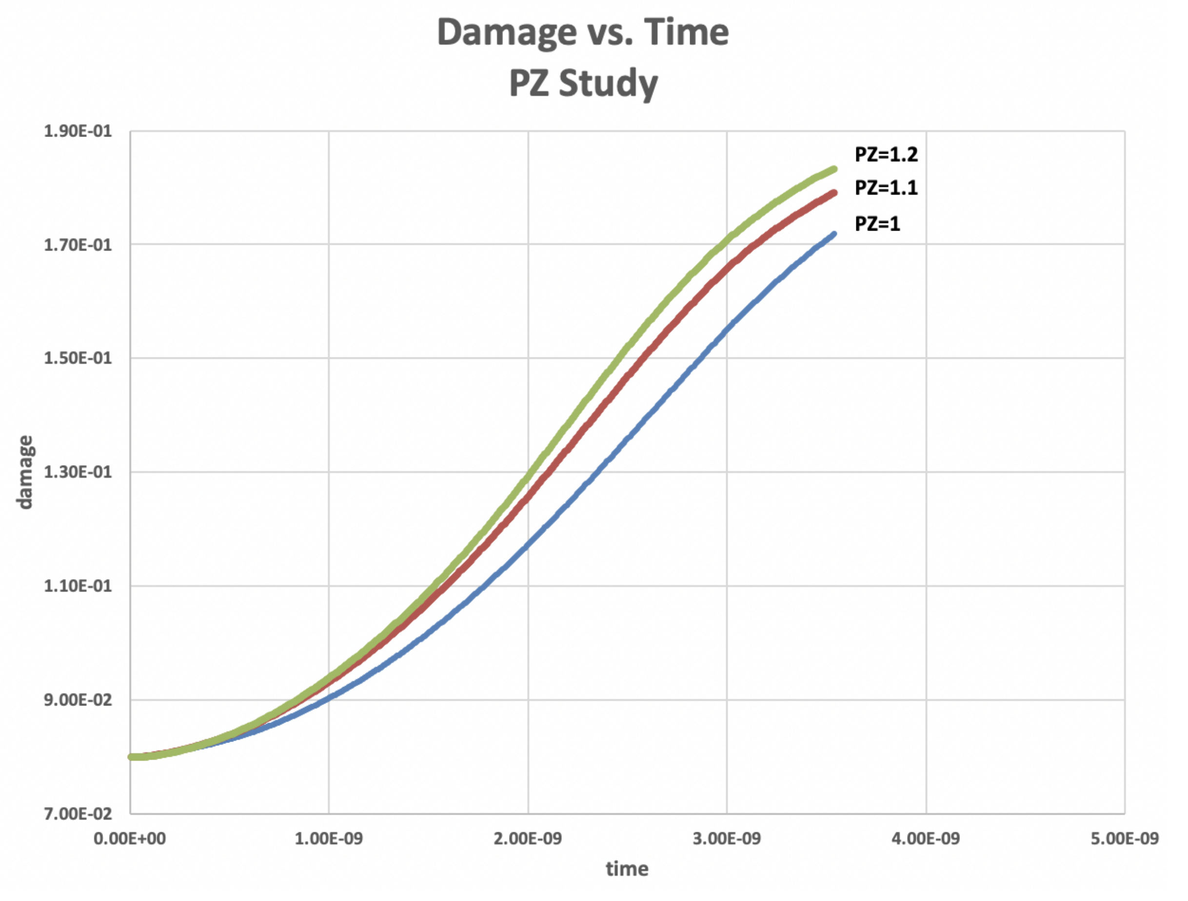
This interaction model has only two new parameters. The process zone is defined to be a fraction of the crack radius. I will explore the sensitivity of in Figure 6 with simulations assuming and . There is relatively small sensitivity since those choices mainly affect time spent in the hotspot phase. The process zone defines the length scales over which two cracks interact, but because it is proportional to the crack size, it does not represent a new length scale.
The second parameter is the maximum initial crack size, which defines a length scale that is the average distance between hotspots in a row. Tying the fracture process to a physical length scale rather than the computational cell size will reduce possible mesh dependence.
3.5. Simulation Parameters
To test the array model, I have used material parameters typical of beryllium. These are listed in Table 1. Beryllium is a material of interest, but is not typical of most other brittle metals; it has a very low Poisson’s ratio and a very high Rayleigh wave speed.
My choice of length scales shown in Table 2 is somewhat arbitrary. I associate the initial crack size distribution with an average grain size of microns. Assuming the exponential size distribution in Equation (8), I choose the maximum crack radius (cutoff radius) to be slightly less than micron; the radius of the maximum crack sets the subcell to be microns. I will define a standard model by setting and to be 100 microns. The relevance of the standard model will become clearer in Section 6 and Section 7 where the effect of the size of the computational cell is discussed. With those choices, the dimensions of the array code then are and . I note in Figure 11 that the number of hotspots in the row that first fails in the is typically between one and two. This is of course a function of the specific choices of length scales.
3.6. Lattice Models and the Array Model
“Disorder and long-range interactions are two of the key components that make material failure an interesting playfield for the application of statistical mechanics. The cornerstone in this respect has been lattice models of the fracture ”[21]
There are many similarities between lattice models and the array model; see [22,23] for reviews of lattice models. The general idea of the lattice model is to discretize a continuum into a lattice in which simple elements, e.g., normal and shear springs or beams, with random properties are connected. A fracture process is initiated by increasing the load until the first element in the lattice fails. To compensate for the failed element, part of the load must be redistributed, increasing the load on most other elements. The redistribution coupled to further increasing load will then cause a second element to fail—and so on. At some point, the process may become self-sustaining, not requiring further increase in load, initiating an avalanche [4].
Beyond the similarities of geometry and randomness, there are also at least two important differences between lattice models and the array model. First, in the lattice model, the constitutive relations are typically linear perfectly elastic. The failure criterion of a lattice element is most often based on either defined critical stress or a critical strain. Simplicity is emphasized in the lattice models [23]. In the array model, crack growth and the associated damage of the elastic moduli is a continuous process. The Griffith criterion [1] associates a different critical stress for each crack size, e.g., the inverse prediction of Equation (1). Significantly, Griffith’s law and Mott’s law introduce length and time scales into the array model. Thus, while the constitutive laws and the failure criterion are more complicated in the array model, they allow scaling laws and are easily implemented.
A second important difference lies in the way the external loading is felt by the elements. In the lattice models, a detailed calculation determines how the load is distributed to each individual element. In the array model, each crack sees the same stress, namely the unique external stress modified by the self-consistent field corrections [2]. The latter picture is consistent with the idea that the array code is representing one computational cell of a finite volume engineering level code. There is essentially no structure or information calculated in the engineering codes at length scales smaller than .
A more quantitative way to distinguish the various length scales in given in [24]. In the array model, is the microscale and defines the representative volume element where microstructure is resolved. is the mesoscale and represents the continuum level where damage and failure are defined. The engineering code, a mesh of finite volume computational cells, represents the macroscale. As noted in the quote from [23], the lattice model is meant for theoretical studies at the level of the microscale. However, there is a class of finite–discrete element codes [25] that has many similarities with lattice codes, while being applicable for engineering scale calculations. For example, the HOSS code (Hybrid Optimization Software Suite) has capabilities for simulation of fracture and fragmentation in general three-dimensional geometries [26].
Remark: I have used the generic term “load” above. The elements of the lattice model, springs and beams, respond to forces that vary from element to element. The cracks in the array model all respond to a unique external stress.
4. The Fracture Process in Words
In all the results of this paper, I will simulate the fracture of a two-dimensional solid with horizontally bedded cracks undergoing normal tension at high strain rates. The fracture process proceeds in three phases, which can be termed elastic, hotspots, and avalanche.
In the initial elastic phase, the tension ramps up but is not sufficient to cause the largest cracks to grow. Recall that the size of the largest cracks is determined by the cutoff I have applied in initializing the crack distribution. When the critical crack size of Equation (1) reduces to that of the largest cracks, the second phase begins. Because those largest cracks represent the extreme of the crack distribution, they are relatively few and can be termed hotspots. With the length scale parameters I have chosen for the simulations, most rows contain no hotspots. A few rows contain one or possibly more. In the hotspot phase, the hotspots grow in isolation under Griffith’s law until the first hotspots intersect their nearest horizontal neighbors—more specifically, when the process zones of the hotspot and nearest neighbor first touch. This initiates the third or avalanche phase in which hotspot(s) continue to grow at the asymptotic speed by the process of coalescence. Ultimately, a crack in one row will span the entire cell, which is the array (mesoscale) definition of failure.
From the point of view of the computational cell, the important quantities are threshold stress for the fracture process to begin, total time to failure, and damage as a function of time. The threshold stress for failure depends directly on our choice of the cutoff crack size. The total time to failure consists of the time spent in the hotspot phase plus the time in the avalanche phase. Since the crack growth in the hotspot phase is an order of the subcell size while the crack growth in the avalanche phase is an order of the total cell , the fracture process in the cell will spend most of its time in the avalanche phase for high strain rate processes. I will qualitatively define high- strain rate processes as those in which most time is spent in the avalanche phase. For lower strain rates, the hotspot cracks will take a longer time to accelerate to the asymptotic growth velocity and to initiate the avalanche process. In the next section, I will consider strain rates of s, s, and s, all of which qualify as high strain rates.
In the avalanche phase, the avalanche moves with the maximum speed, i.e., the Rayleigh wave speed, cf. Equation (4), which depends on the material properties, but is independent of the strain rate. On the other hand, the total damage in the computational cell is dominated by the growth of cracks in all the rows, of which the damage in the particular row that fails is only a small part. One should expect that the total damage at the time of failure will depend on strain rate. A higher strain rate implies faster growth of the stress field and faster decrease of the critical crack size from Equation (1). In other words, a higher strain rate implies more cracks will grow in the avalanche phase and cause a larger value of damage at time of failure.
Note that the time spent in the avalanche phase depends in a discontinuous fashion on the number of hotspots in the row that causes failure, which should be understood in terms of extreme statistics. One might expect that the time to failure for a row with two hotspots would be, roughly speaking, only half that of a row with one hotspot. Then the growth of the totality of subcells and the resulting damage in the case of two hotspots would be much less than in the case of one hotspot. Will averaging over an ensemble of failure processes with these bimodal, or perhaps multimodal statistics lead to smooth results for the damage as a function of time, or for final damage at the time of failure? If so, how many processes must one consider in the ensemble?
These questions can be readily answered by the array code in the next section. The significant difference between the growth of damage for a particular, but arbitrarily chosen realization in which one hotspot exists versus a different (arbitrarily chosen) realization in which two hotspots exist is illustrated in Figure 1. The ensemble-averaged result for one hundred realizations lies between the single realization cases.
5. The Fracture Process in Graphs
Here I illustrate with graphs the fracture process as described by the array code. All the results in this section are based on the standard model , specifically for the finite volume cell μm. The base set of parameters for most calculations in this section uses an ensemble of 100 runs, each differing only in the initial realization of the crack sizes and locations, All simulations of the ensemble employ the interaction fracture model, most with a process zone length that is of the crack radius.
5.1. Damage vs. Time
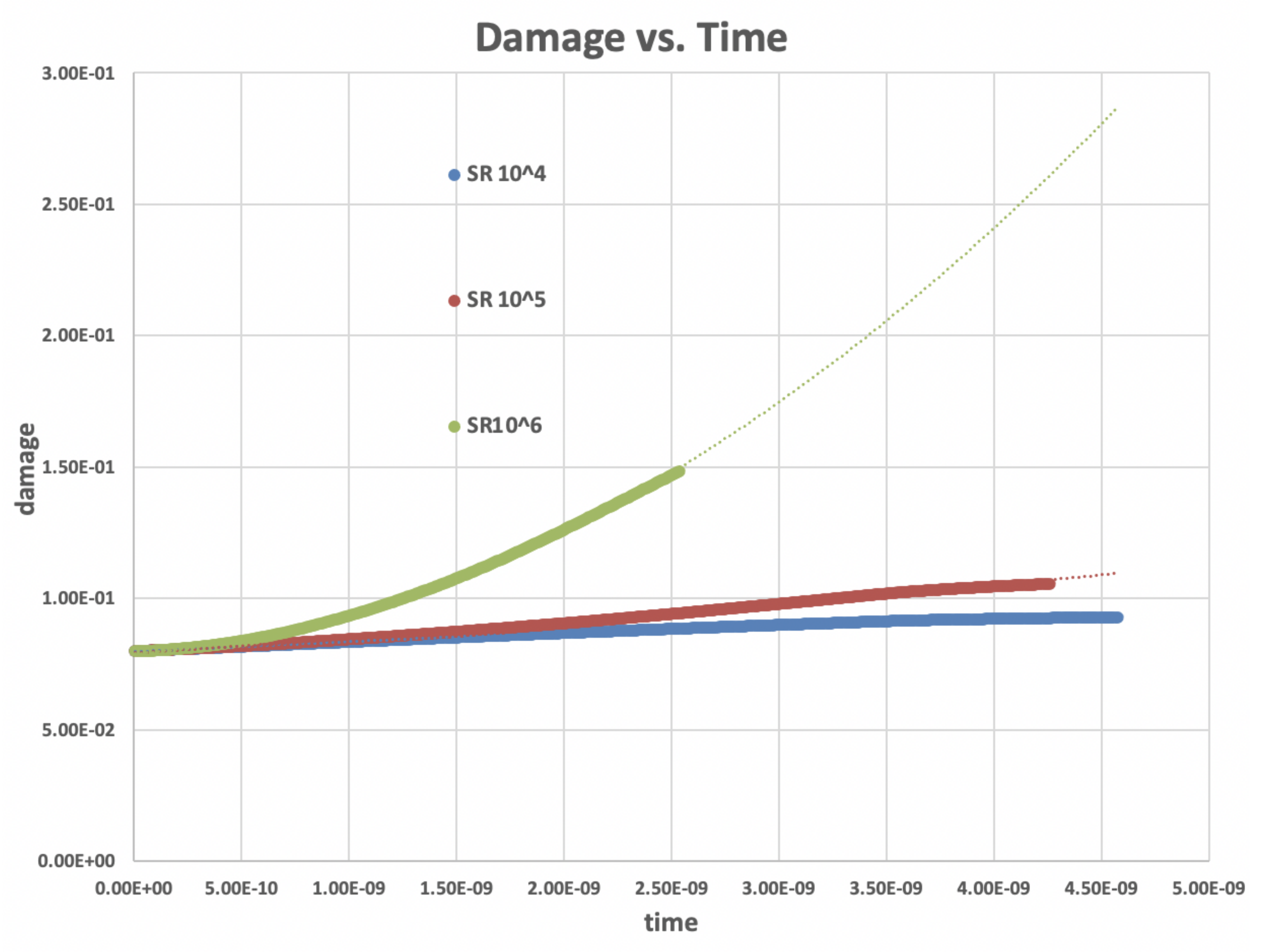
In Figure 2 the time evolution of the damage, averaged over the 100 runs of the ensemble, is plotted versus time. The damage is , defined in Equation (7). The time is measured from the beginning of the avalanche phase. The three curves represent results of three strain rates, s, s and s. The graph shows that the higher the strain rate, the faster the damage accumulates and the higher the value of damage at the time of failure. Trendlines show highly accurate fits by second-order polynomials in time for each of the curves.
Each of those cases lies in the regime previously termed high strain rates. However, the curves are further distinguished by the relative contributions of the linear and the quadratic terms of the trendline polynomial; the curve corresponding to s represents the transition where both terms are approximately equal. The coefficient of the quadratic term depends on the square of the strain rate from dimensional considerations; similarly the coefficient of the linear term is proportional to the strain rate. The constant term represents the initial damage, which has been postulated to be a material property.
Assuming the continuous behavior of damage in its dependence on time and strain rate, it is then possible to determine a curve representing the evolution of damage in the for any strain rate as a function of time from just three dimensionless numbers. Those numbers will depend on the details of the array model and can be readily extracted from the array code.
5.2. Time to Failure, Damage and Stress vs. Strain Rate
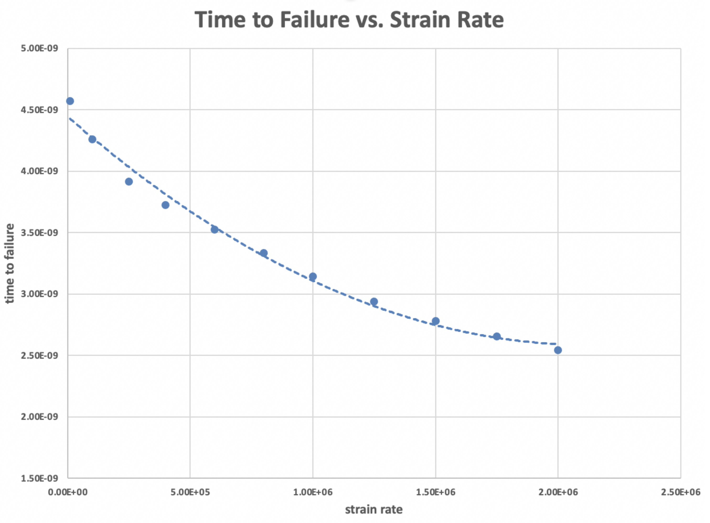
In Figure 3, time to failure measured from the beginning of the avalanche phase is plotted versus strain rate. Failure has been defined as the first propagation of a crack completely across the cell. The curve shows the monotonic decrease of the interval time as strain rate increases. This curve is accurately fit by a polynomial second-order in strain rate. The coefficients of that polynomial are constants for the and can be extracted from the array code.
Whereas the curve of Figure 2 describes the accumulation of damage, the additional input of Figure 3 is required to determine when damage ceases to grow. The direct relation between damage at time of failure and strain rate is exhibited in Figure 4. That curve is also accurately fit by a second-order polynomial in the strain rate.
In principle, the residual stress left in the separate pieces of the fractured cell can be calculated directly by the finite volume computational cell, given the elastic moduli, the damage and the strain rate. However, when fracture proceeds rapidly, i.e., within a few computational cycles, that calculation may be inaccurate. The calculation within the array code proceeds at a much smaller time step and would be more accurate in the absence of interactions between the computational cell and its neighbors. In Figure 5, the stress at time of failure, for all the calculations in this paper, is plotted versus strain rate. Although the graph shows a monotonic growth of the residual stress with strain rate, the growth is very small and is likely insignificant.
5.3. Sensitivity
In Figure 6, the sensitivity of the model to three choices of process zones (PZ) is explored by plotting the evolution of damage in time. The three curves represent process zones that are , and of the crack radius. The process zone determines when neighboring cracks may begin to interact. Despite choices that represent a significant fraction of the crack radius itself, the sensitivity is small. The damage at time of failure differs by much less than and the residual stress shows even less sensitivity. The time to failure does show larger sensitivity, since the process zone effectively makes the cracks bigger.
The sensitivity to ensemble size was tested by running the at a strain rate of s for ensembles of 100, 200, and 500 members. No sensitivity was seen at the level of .
5.4. Qualitative Summary of Graphs
Beyond the quantitative results exhibited in the graphs, one may formulate the following qualitative conclusions:
- Despite the bimodal or multimodal nature of hotspots, the ensemble-averaged curves of damage versus time and versus strain-rate are continuous and smooth. They can replace detailed knowledge of the evolving crack distribution greatly simplifying the SCM.
- Further, the scaling laws are relatively simple and invariant (in form) over more than 3 decades of strain rates.
- Values of damage at failure are much less than would be predicted by the percolation thresholds. The long range effect of the entire spectrum of cracks is small and dominated by the local effect of nearest neighbors. Typical percolation thresholds occur at damage levels of , see [27], whereas Figure 4 shows failure occurring in the array model with crack interactions at damage levels .
- There is relatively small uncertainty due to the assumed size of the process zone. There is also small uncertainty to the size of the ensemble beyond the minimum of 100 used as a baseline in the simulations reported. Further, even the ensemble of 500 simulations of our two-dimensional problems took only a few minutes on an Apple workstation.
- I have not systematically explored the uncertainty of our results to the choice of the maximum crack size. The direct relation of stress at failure to the maximum crack size suggests that this parameter may be effectively deduced from experimental data. I have chosen the maximum crack size to be four times the average crack size in the exponential distribution, Equation (8). A smaller maximum would mean more hotspots and perhaps imply qualitative changes in the fracture process.
6. Size Effect
All of the numerical experiments of the previous section were performed on a finite volume computational cell with dimensions 100 microns by 100 microns. Do the various scaling relations derived there depend on the actual size or shape of the cell? It is straightforward to test this in the array code by varying and while keeping all other length scales, e.g., , , , unchanged. In this section, all the simulations assume a constant applied strain rate of s.
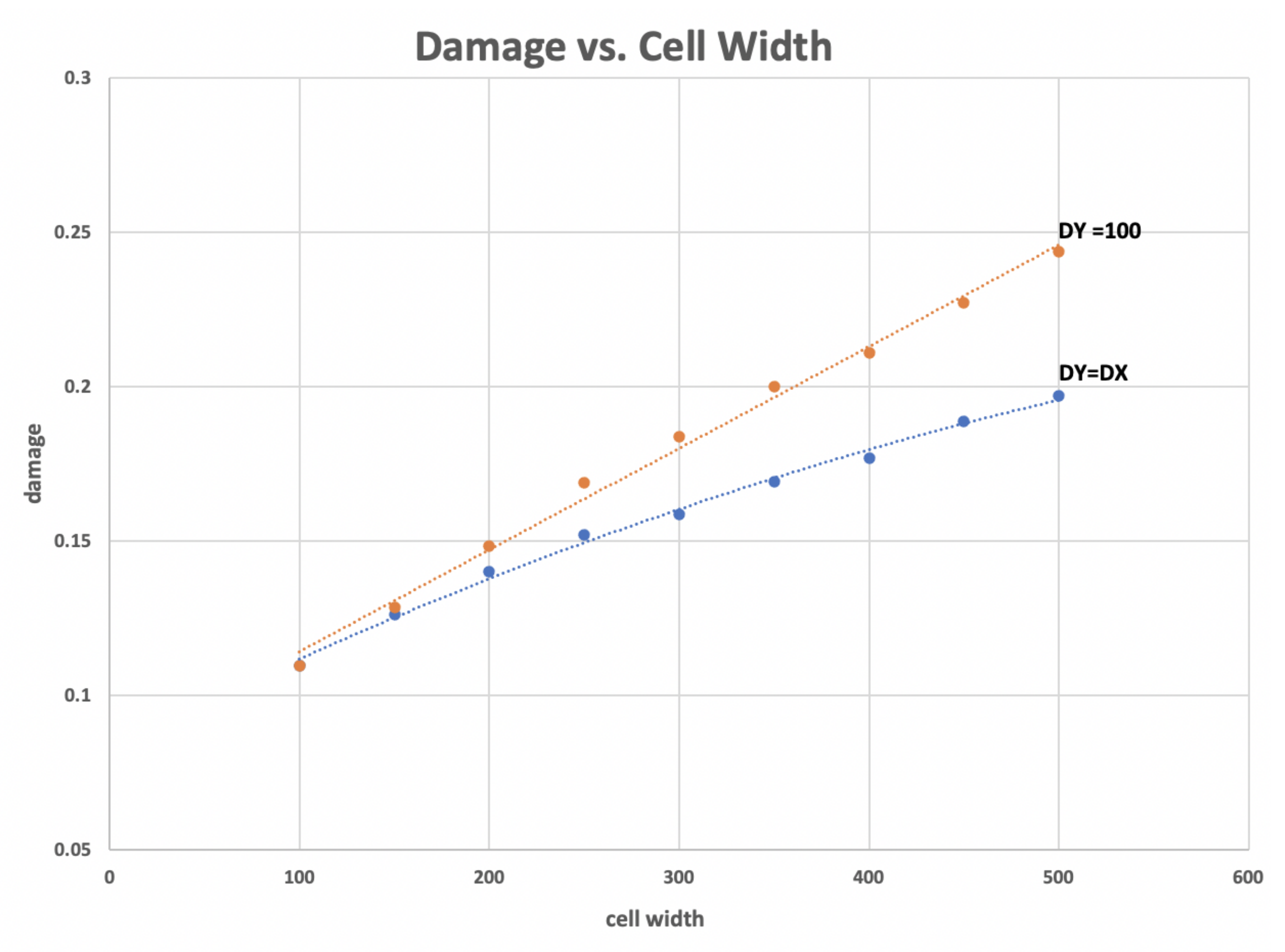
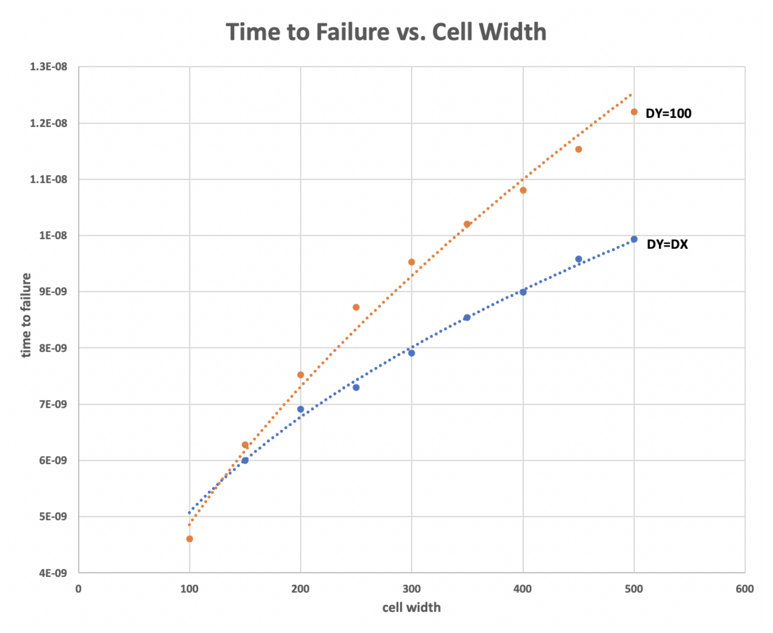
Figure 7 and Figure 8 show array code results for the dependence of time to failure and of damage at time of failure for two variations of cell size. In one variation, the cell remains square so that . In the second variation, only varies while μm. The point at μ is common to both sets of data. The graphed results show a systematic increase in the apparent strength of the larger computational cells, as defined by the level of damage that can be supported before failure; that is the case for both variations of increasing the cell size. Further, each of the four curves in those figures can be accurately modeled by a scale-invariant power law, which is shown on the graph. Both figures also show that the thinner cells, i.e., where are stronger than the square cells where .
Figure 7 and Figure 8 imply that in addition to the size effect, there is a shape effect. However, Table 3 shows that both the time to failure and the damage at time of failure are much more sensitive to varying the width than they are to varying the height.
When considering discrete physical samples, it is well known that bigger samples are weaker than smaller samples. That result is understood from the argument that (1) bigger cracks begin to grow at lower stress levels; and (2) bigger samples are more likely to contain bigger cracks. However, that argument does not apply to the array model where I have limited the radius of the largest crack to which remains constant in the simulations.
The apparent strength of wider samples lies in the assumed hotspot nature of the fracture process and the details of the interaction model in the array code. It is illustrative to consider how those details lead to the result that wider cells are stronger.
- In the array code, one calculates an ensemble of fracture processes, each with a different realization of the cracks seeded.
- Cracks are assumed to grow with the Rayleigh wave speed in the avalanche phase. Thus, the time to failure for any individual fracture process is roughly determined by the largest actual distance (gap) between hotspots found in the critical row, i.e., in the row or rows that have the maximum number of hotspots among all the rows of the computational cell.
- The largest distance between hotspots in the critical row is limited by the size of the computational cell.
- A mathematical calculation of the conditional probabilities involved would be a monumental task. However, the array code is easily able to generate the statistics. The important issue is to consider sufficient processes in the ensemble to ensure that the statistics have converged.
Summary: bigger computational cells are more likely to have bigger gaps between hotspots. This implies longer times to failure and higher levels of damage at failure.
7. Scaling the Standard Model
The primary task of the SCM is to predict damage and failure as a function of the loading. The size effect described in the previous section would appear to complicate the prediction of failure as it might seem that a new “standard” model is required for every size and shape (aspect ratio) of a computational cell. In this section, I will consider variations of the width of and ignore the smaller effects of not having square cells, cf. Table 3.
Figure 9 shows the accumulation of damage as a function of time for 4 square cells of dimensions , , and (all units in microns). The strain rate is s. The circles represent the individual times of failure of the four cells, with larger cells showing more damage at the time of failure. The notable feature is that the damage growth in all cells is described by the same “backbone” curve. That is, for fracture at s, the increase of damage in time follows the quadratic curve in Figure 9 until time of failure for all square cells, . A plot (not shown) for all cells with μm is qualitatively similar, i.e., damage increases for all cells on a slightly different backbone quadratic curve until time of failure.
Perhaps the most surprising result can be seen in Figure 10, where data of damage vs. time to failure for both shapes of cells are combined in a single plot. The resulting curve is a single straight line. Further, additional data for a wide variety of cell sizes and shapes also lie on the same straight line. To summarize, there is a linear relationship between damage and time to failure for all cells fracturing at a strain rate of s. Similar linear relationships will exist for all high strain rate processes and the slope of the line will, for dimensional reasons, depend linearly on the strain rate.
To implement the for cells of arbitrary width, first, recall that the relevant curves in Figure 7, Figure 8, Figure 9 and Figure 10 are all fit by simple polynomials whose coefficients are readily scaled for any strain rate. Now suppose one is given the strain rate and the width of the cell. From the curve in Figure 4, one finds the damage at time of failure for a cell with width μm. Then, from the (lower) curve in Figure 7, scaled to the given strain rate, one finds the damage at time of failure for a cell of the given width. The time to failure of the cell is then found from the (scaled) curve in Figure 10. Finally, the damage as a function of time is given in the (scaled) curve of Figure 9. In practice, all these steps can be composed.
8. Summary and Discussion
“The mistake is thinking that there can be an antidote to the uncertainty.”David Levithan
In this paper, I have taken a close look at a statistical crack model (SCM) with the object of introducing a model of crack interactions (coalescence) and understanding the qualitative changes it induces in the fracture process. Fracture is a statistical process when viewed at the continuum level, which depends on details of microstructure that cannot be known in full. The philosophy of the SCM is to introduce simple microphysical models that contain the appropriate scales of length and time. In Section 2, I summarized the models of a particular program, the BCM [9]. In Section 3, I described a new tool for studying the behavior of BCM; the array code is a computer program in which the microphysical models of the BCM are implemented to simulate the growth a randomly generated array of microcracks. This array code is a realization of a single finite volume computer cell in an engineering scale simulation program.
In addition to the physics of BCM, I implemented a new model for microcrack interactions. In Section 4 and Section 5, I used the array code to generate statistics of the fracture process, including the evolution of damage and failure. Fracture is initiated by only a few cracks in each realization, namely the largest cracks in the extreme tail of the size distribution. Those largest cracks are like hotspots, perhaps one or two or three in each realization. Thus the statistics are multimodal; however, the ensemble-averaged statistics of damage evolution, damage at time of failure and time to failure are smooth functions of time and applied strain rate, with scaling described by low-order polynomials.
The major modification to the SCM is the elimination of the need to evolve the statistical distribution of crack sizes. It should be noted that this simplification is not dependent on the introduction of the crack interaction model, but works as well for the original BCM. Indeed, that was the original motivation for building the array code.
The most important modification to the description of the fracture process is that precise definitions of damage and failure lead to a prediction of failure as a function of damage. The relation is not constant and does not depend on identifying the percolation threshold of the effective elastic moduli with failure. Indeed, failure takes place at much lower levels of damage, consistent with experimental data [5,6]. That result leads to reconsidering aspects of how an SCM is implemented.
- Time to failure is much shorter: In the avalanche phase, the crack that causes failure grows with the Rayleigh wave speed, cf. Equation (4). Dividing the cell width by that speed produces a time interval characteristic of the fracture process, perhaps even made shorter if several hotspots are present in the row that fails. Independently, that time scale is also the maximum time step allowed by the Courant–Friedrichs–Lewy stability condition for explicit dynamics in a finite volume engineering code. To properly resolve the interactions between computational cells, it will probably be necessary to either subcycle the fracture process or to treat it implicitly.
- There is residual stress at failure: That failure occurs at a low level of damage also implies that there is residual stress present in the cell at the time of failure. This is shown explicitly in Figure 5. Residual stress means residual strain, which must be distributed to the neighboring cells.
- Diffusion of damage: Although crack growth ends at the cell boundaries in the array code, it will continue across cell boundaries in the finite volume engineering codes. This modification can be modeled in detail in the array code to inform a macroscopic diffusion process.
I will close with one final thought. Fracture is not only a statistical process, it is a stochastic process. In Figure 11, it is shown that the number of hotspots in a standard cell is . This is an expectation value; in the 100 ensemble runs that generated that result, 94 runs had one hotspot and six runs had two hotspots. It would be possible to work out the statistics of damage, time to failure, damage at failure and for time to failure separately for an ensemble in which only one hotspot appears, and separately for an ensemble in which two (or more) hotspots appear. An explicit example is shown in Figure 1. These would represent different models. Then in the engineering code, one could randomly assign one or the other of these models to the cells with appropriate probability. The necessary statistics could be easily generated in the array code.
“To travel hopefully is better than to arrive.”(James Jeans)
Funding
This research received no external funding.
Acknowledgments
I dedicate this paper to my friend and colleague Lynn Seaman (1933–2007). This research and these ideas all started with you. I acknowledge interesting discussions with A. Hunter, D. Burton, M. Ostoja-Starzewski and C.W. Hirt. I appreciate the support of the Physics and Engineering Models project of the ASC program. This work was performed under the auspices of the U.S. Department of Energy’s NNSA by the Los Alamos National Laboratory, is managed by Triad National Security, LLC for the National Nuclear Security Administration of the U.S. Department of Energy under contract 89233218CNA000001.
Conflicts of Interest
The authors declare no conflict of interest.
References
- Margolin, L.G. A generalized Griffith criterion for crack propagation. Eng. Fract. Mech. 1984, 19, 539–543. [Google Scholar] [CrossRef]
- Hoenig, A. Elastic moduli of a non–randomly cracked body. Int. J. Solids Struct. 1979, 15, 137–154. [Google Scholar] [CrossRef]
- Mott, N.F. Brittle fracture in mild steel plates. Engineering 1948, 165, 16–18. [Google Scholar]
- Zapperi, S.; Kumar, P.; Nukala, V.V.; Simunovic, S. Crack avalanches in the three–dimensional random fuse model. Phys. A 2005, 357, 129–133. [Google Scholar] [CrossRef] [Green Version]
- Guégue, Y.; Chelidze, T.; Ravalec, M.L. Microstructures, percolation thresholds, and rock physical properties. Tectonophysics 1997, 279, 23–35. [Google Scholar] [CrossRef]
- Kachanov, M. Elastic solids with many cracks and related problems. Adv. Appl. Mech. 1994, 30, 259–445. [Google Scholar]
- Bdzil, J.B.; Aslam, T.D.; Henninger, R.; Quirk, J.J. High–Explosives Performance. Los Alamos Sci. 2003, 28, 96–110. [Google Scholar]
- Dienes, J.K. A statistical theory of fragmentation processes. Mech. Mater. 1978, 4, 325–335. [Google Scholar] [CrossRef] [Green Version]
- Margolin, L.G. Microphysical models for inelastic material response. Int. J. Eng. Sci. 1984, 22, 1171–1179. [Google Scholar] [CrossRef]
- Seaman, L.; Curran, D.R.; Shockey, D.A. Computational models for ductile and brittle-fracture. J. App. Phys. 1976, 47, 4814–4826. [Google Scholar] [CrossRef]
- Curran, D.R.; Seaman, L. Simplified models of fracture and fragmentation. In High–Pressure Shock Compression of Solids; Davison, L., Shahinpoor, D.G.M., Eds.; Springer: New York, NY, USA, 1996; pp. 340–365. [Google Scholar]
- Seaman, L.; Shockey, D.A. Models for ductile and brittle fracture for two–dimensional wave propagation calculations. In Stanford Research Laboratory Report AMMRC CTR 75-2; Army Materials and Mechanics Research Center: Watertown, MA, USA, 1975. [Google Scholar]
- Griffith, A.A. Phenomena of rupture and flow in solids. Phil. Trans. R. Soc. A 1920, 221, 163–198. [Google Scholar]
- Craggs, J.W. On the propagation of a crack in an elastic–brittle material. J. Mech. Phys. Solids 1960, 8, 66–75. [Google Scholar] [CrossRef]
- Willis, J.R. Crack propagation in viscoelastic media. J. Mech. Phys. Solids 1967, 15, 229–240. [Google Scholar] [CrossRef]
- Margolin, L.G. Effective moduli of a cracked body. Int. J. Fract. 1984, 22, 65–79. [Google Scholar] [CrossRef]
- Bazant, Z.P. Size effect. Int. J. Solids Struct. 2000, 37, 69–80. [Google Scholar] [CrossRef]
- Abraham, F.F.; Gao, H. How fast can cracks propagate. Phys. Rev. Lett. 2000, 84, 3113–3116. [Google Scholar] [CrossRef] [PubMed] [Green Version]
- Krajcinovic, D. Damage Mechanics; North Holland: Amsterdam, The Nederlands, 1996. [Google Scholar]
- Zubelelewicz, A.; Rougier, E.; Ostoja–Starzewski, M.; Knight, E.E.; Bradley, C.; Viswanathan, S. A mechanism–based model for dynamic behavior and fracture of geomaterials. Int. J. Rock Mech. Min. Sci. 2014, 72, 277–282. [Google Scholar] [CrossRef] [Green Version]
- Alava, M.J.; Nukala, P.K.; Zapper, S. Statistical models of fracture. Adv. Phys. 2006, 55, 349–476. [Google Scholar] [CrossRef] [Green Version]
- Ostoja–Starzewski, M. Lattice models in micromechanics. Appl. Mech. Rev. 2002, 55, 35–60. [Google Scholar] [CrossRef]
- Pan, Z.; Ma, E.; Wang, S.; Chen, A. A review of lattice type model in fracture mechanics: Theory, applications and perspectives. Eng. Frac. Mech. 2018, 190, 382–409. [Google Scholar] [CrossRef]
- Ostoja–Starzewski, M. Material spatial randomness: From statistical to representative volume element. Probabilistic Eng. Mech. 2006, 21, 112–132. [Google Scholar] [CrossRef]
- Munjiza, A.A.; Knight, E.E.; Rougier, E. Computational Mechanics of Discontinua; John Wiley & Sons: Hoboken, NJ, USA, 2015. [Google Scholar]
- Knight, E.E.; Rougier, E.; Lei, Z.; Euser, B.; Chau, V.; Boyce, S.H.; Gao, K.; Okubo, K.; Froment, M. HOSS: An implementation of the combined finite–discrete element method. Comput. Part. Mech. 2020, 7, 1–23. [Google Scholar] [CrossRef]
- Budiansky, B.; O’Connell, R.J. Elastic moduli of a cracked solid. Int. J. Solids Struct. 1976, 12, 81–97. [Google Scholar] [CrossRef]
Figure 1.
The time rate of accumulated damage is compared for two realizations, one in which one hotspot initially exists and the second in which two hotspots initially exist. The dotted curve represents the average of an ensemble of 100 realizations. All simulations were performed for a strain rate s; m. The process zone is 10% of the crack radius. The particular realizations were chosen randomly from the ensemble.

Figure 2.
The ensemble-averaged damage is plotted as a function of time for 3 imposed strain rates, s s and s. The ensemble size is 100 and the process zone is 10% of the crack radius. The data is captured by a quadratic trendline with an in each case. Higher strain rates lead to shorter times to failure and more damage at time of failure.

Figure 3.
The ensemble-averaged time to failure is plotted as a function of strain rate. The ensemble size is 100 and the process zone is 10% of the crack radius. The time to failure decreases monotonically with strain rate and the curve is captured by a quadratic trendline with .
Figure 3.
The ensemble-averaged time to failure is plotted as a function of strain rate. The ensemble size is 100 and the process zone is 10% of the crack radius. The time to failure decreases monotonically with strain rate and the curve is captured by a quadratic trendline with .

Figure 4.
The damage at the time of failure is plotted as a function of strain rate. The ensemble size is 100 and the process zone is 10% of the crack radius. Higher strain rates lead to more damage sustained at the time of failure. The curve is captured by a quadratic trendline with .
Figure 4.
The damage at the time of failure is plotted as a function of strain rate. The ensemble size is 100 and the process zone is 10% of the crack radius. Higher strain rates lead to more damage sustained at the time of failure. The curve is captured by a quadratic trendline with .

Figure 5.
The stress component at time of failure is plotted vs. strain rate. The ensemble size is 100 and the process zone is 10% of the crack radius. That stress increases slightly with strain rate, but is essentially constant. The curve is captured by a quadratic trendline with .
Figure 5.
The stress component at time of failure is plotted vs. strain rate. The ensemble size is 100 and the process zone is 10% of the crack radius. That stress increases slightly with strain rate, but is essentially constant. The curve is captured by a quadratic trendline with .

Figure 6.
The ensemble-averaged damage is plotted as a function of time for an imposed strain rate s. The three curves represent process zone sizes of , and of the crack radius. The ensemble size is 100. A larger process zone implies slightly more damage at time of failure.
Figure 6.
The ensemble-averaged damage is plotted as a function of time for an imposed strain rate s. The three curves represent process zone sizes of , and of the crack radius. The ensemble size is 100. A larger process zone implies slightly more damage at time of failure.

Figure 7.
Damage at time of failure is plotted as a function of the cell width . The strain rate for all points is s, the ensemble size is 100 and the process zones is of the crack radius. In the upper curve, μm for all points. In the lower curve, . On both curves, wider cells support more damage at failure. Taller cells support less damage at failure.

Figure 8.
Time of failure is plotted as a function of the cell width . The strain rate for all points is s, the ensemble size is 100 and the process zones is of the crack radius. In the upper curve, μm for all points. In the lower curve, . On both curves, wider cells take longer times to fail. Taller cells take less time.

Figure 9.
The ensemble-averaged damage is plotted as a function of time for an imposed strain rate s, an ensemble size of 100 and the process zone is of crack radius. The four dots represent damage at time of failure for μm and . The damage backbone is the same for all cell widths, but the time to failure increases with the cell width.

Figure 10.
Damage at time of failure is plotted versus time to failure for s, an ensemble size of 50 and the process zone is of crack radius. This plot is a synthesis of the data in Figure 7 and Figure 8 when cell width is eliminated. The curve shows points representing both shapes fall on the same straight line.

Figure 11.
The ensemble-averaged number of hotspots contained in the most critical row (the row that causes failure of the cell) is plotted as a function of cell width. The upper curve has square cells while the lower curve has μm. All points are calculated with an imposed strain rate s, an ensemble size of 100 and the process zone is of the crack radius. The curves are linear in the cell width, indicating that the average distance between hotspots is constant as a function of width. However, the taller cells sample more rows and the critical row will probably contain more hotspots.


Table 1.
Material parameters simulating beryllium.
| Shear modulus G | kbar |
| Bulk modulus B | kbar |
| Poisson ratio | |
| Youngs modulus E | kbar |
| First Lamé modulus | kbar |
| Rayleigh wave speed v | km/s |
| Cell DX | 100 μm |
Table 2.
Length scales.
| Cell DX | 100 μm |
| Subcell dx | 1 μm |
| Average crack radius | μm |
| Max crack radius | μm |
Table 3.
Doubling the width of the statistical crack model () () leads to large changes in the time to failure and damage at failure. Doubling the height of the leads to much smaller changes in both quantities.
Table 3.
Doubling the width of the statistical crack model () () leads to large changes in the time to failure and damage at failure. Doubling the height of the leads to much smaller changes in both quantities.
| Cell I,J | Time to failure (s) | Damage |
Publisher’s Note: MDPI stays neutral with regard to jurisdictional claims in published maps and institutional affiliations. |
© 2020 by the author. Licensee MDPI, Basel, Switzerland. This article is an open access article distributed under the terms and conditions of the Creative Commons Attribution (CC BY) license (http://creativecommons.org/licenses/by/4.0/).
Share and Cite
MDPI and ACS Style
Margolin, L.G. Damage and Failure in a Statistical Crack Model. Appl. Sci. 2020, 10, 8700. https://doi.org/10.3390/app10238700
AMA Style
Margolin LG. Damage and Failure in a Statistical Crack Model. Applied Sciences. 2020; 10(23):8700. https://doi.org/10.3390/app10238700
Chicago/Turabian StyleMargolin, L.G. 2020. "Damage and Failure in a Statistical Crack Model" Applied Sciences 10, no. 23: 8700. https://doi.org/10.3390/app10238700
Note that from the first issue of 2016, this journal uses article numbers instead of page numbers. See further details here.