Real-Time Physical Activity Recognition on Smart Mobile Devices Using Convolutional Neural Networks

Abstract

Given the ubiquity of mobile devices, understanding the context of human activity with non-intrusive solutions is of great value. A novel deep neural network model is proposed, which combines feature extraction and convolutional layers, able to recognize human physical activity in real-time from tri-axial accelerometer data when run on a mobile device. It uses a two-layer convolutional neural network to extract local features, which are combined with 40 statistical features and are fed to a fully-connected layer. It improves the classification performance, while it takes up 5–8 times less storage space and outputs more than double the throughput of the current state-of-the-art user-independent implementation on the Wireless Sensor Data Mining (WISDM) dataset. It achieves 94.18% classification accuracy on a 10-fold user-independent cross-validation of the WISDM dataset. The model is further tested on the Actitracker dataset, achieving 79.12% accuracy, while the size and throughput of the model are evaluated on a mobile device.

1. Introduction

Human Activity Recognition (HAR) is an active area of research, since it can automatically provide valuable knowledge and context about the actions of a person using sensor input. Its importance is evidenced by the variety of the areas it is applied to, including pervasive and mobile computing [1,2], context-aware computing [3,4,5], sports [6,7], health [8,9], elderly care [9,10], and ambient assisted living [11,12,13]. In recent years, there has been a growing interest in the field, because of the increase of the availability of low-cost and low-power sensors, especially the ones embedded in mobile devices, along with the improvement of the data processing techniques. This growing interest can also be attributed to the increasingly aging population [14] in the case of health and elderly care applications.

At the same time, several datasets have been collected over the years, including a range of modalities [15]. There has been a great contribution from human activity recognition video datasets; some of the most important include the 20BN-something-something Dataset V2 [16], VLOG [17], and EPIC-KITCHENS [18]. However, using video datasets for activity recognition entails potential pitfalls. Compared to using inertial sensors, there is a greater risk of violating personal data; they require a camera setup or a person actively recording the video at runtime, and their processing is heavier. The ubiquity of mobile devices and their embedded sensors have produced a multitude of datasets, which include accelerometer, gyroscope, magnetometer, and ECG data, such as the MHEALTH [19,20], the OPPORTUNITY Activity Recognition [21], the PAMAP2 [22], the USC-HAD [23], the UTD-MHAD [24], the WHARF [25], the WISDM [26], and the Actitracker [27] datasets. A wide range of sensors has been also used to create Adaptive Assisted Living (AAL) HAR datasets, including reed switches, pressure mats, float sensors, and Passive Infrared (PIR) sensors [28].

In the context of human physical activity recognition, competitive performance can also be achieved using only the input data from a mobile device’s sensors. This offers potential unobtrusiveness and flexibility, but also introduces a number of challenges [29]. The motion patterns are highly subject dependent, which means that the results are heavily affected by the subjects participating in the training and testing stages. The activity complexity increases the difficulty of the recognition either because of multiple transitions between different motions or because of performing multiple activities at the same time. Energy and resource constraints should also be considered, since the capacity of mobile devices is limited, and demanding implementations will drain their battery. Localization is important to understand the context of a situation, but implementing it using GPS is problematic in indoor environments, while inferring distance covered with motion sensors usually results in the accumulation errors over time. Of course, it is also crucial to adapt research implementations to real-life problems, such as elderly care, workers’ ergonomics, youth care, and assistance for disabled people. At the same time, the privacy of sensitive data collected from the subjects must always be respected and protected, even at the expense of a solution’s performance.

The conventional method to extract knowledge from these datasets is with machine learning algorithms such as decision tree, support vector machine, naive Bayes, and hidden Markov models [30]. They perform well in specific cases, but rely on domain-specific feature extraction and do not generalize well easily [31]. Contrary to machine learning methods, deep learning methods perform the feature extraction automatically, and specifically, Convolutional Neural Networks (CNN), which are also translation invariant, have achieved state-of-the-art performance in many such tasks [15].

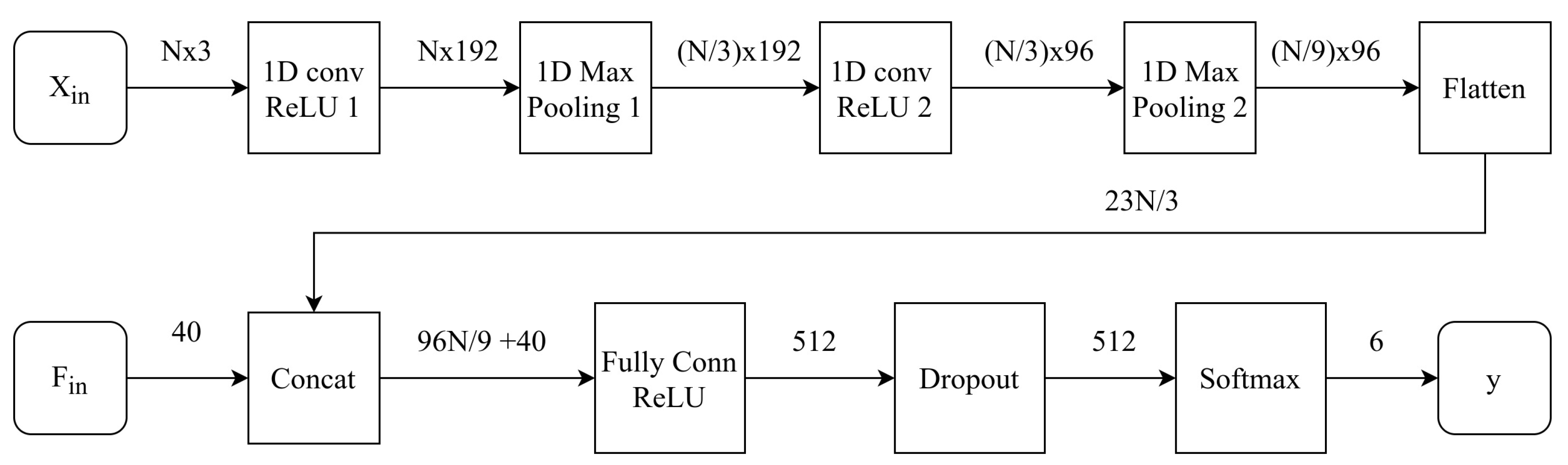
In this paper, a CNN model is proposed, which takes as the input raw tri-axial accelerometer data and passes them through the 1D convolutional and max-pooling layers. These layers effectively extract local and translation-invariant features in an unsupervised manner. The output of these layers is concatenated with an input of 40 statistical features, which supplement the previous with global characteristics. These are passed through a fully-connected and softmax layer to perform the classification. The model is trained and tested on two public HAR datasets, WISDM [26] and Actitracker [27], achieving state-of-the-art performance. Finally, the model is tested online on a mobile device, performing in real time, measuring and presenting significantly improved throughput and reduced size.

The remainder of this paper is structured as follows: Section 2 summarizes the related work. Section 3 presents the proposed solution, datasets, and metrics. Section 4 describes the experimental setup and presents the results, and Section 5 concludes this paper and proposes future improvements.

2. Related Work

Traditionally, machine learning approaches were followed in order to achieve human activity recognition [32]. Decision trees are preferred because of their interpretability and low computational cost compared to more complex models [30]. The J48 algorithm is an open source Java implementation of the C4.5 decision tree algorithm in [33] and is usually used for HAR from motion sensor data, using features extracted by time domain wave analysis [34] or statistical features [26]. Other popular classifiers also used for HAR from motion sensor data are K-nearest neighbors and Support Vector Machines (SVMs). K-nearest neighbor classifiers were used with raw accelerometer data and shown to be inferior to using a CNN [35], while Tharwat et al. [36] used particle swarm optimization to produce an optimized k-NN classier. K-nearest neighbor is an Instance Based Learning (IBL) algorithm, which is relatively computationally expensive because it requires the comparison of the incoming instance with every single training instance. However, it offers the ability to adapt to new data and eliminate old data easily. Using an implementation of SVMs that does not require much processing power and memory, six indoor activities were recognized with an accuracy of 89% in [37]. Ensemble classifiers, such as the bagging and boosting ensemble meta-algorithms [3,38], combine the outputs of several classifiers of the same type in order to get better results. On the other side, ensemble algorithms are more computationally expensive, since more base level algorithms need to be trained and evaluated [30].

The state-of-the art performance of deep learning methods has been reported in various works coming from different approaches. For example, Hammerla et al. [39] used a bi-directional Long Short-Term Memory (LSTM), which contains two parallel recurrent layers that stretch both into the “future” and into the “past”, to achieve a 92.7% f1-score on the Opportunity dataset [21], while a combination of convolutional and recurrent layers, named DeepConvLSTM, was used by Ordonez et al. [40], achieving 95.8% accuracy on the Skoda dataset [41]. However, both of the above datasets require multiple wearable sensors, which enable the recognition of more complex activities, but also render the approach more intrusive.

This work will focus on non-intrusive implementations, where data coming only from a mobile device’s sensors are used. A commonly used dataset is the UCI HAR dataset [42] with a waist-mounted mobile device. Using its embedded accelerometer and gyroscope, three-axial linear acceleration and three-axial angular velocity were captured at a constant rate of 50 Hz. It was partitioned into two sets, where 70% of the volunteers were selected for generating the training data and 30% for generating the test data, which standardized the results of the implementations. Sikder et al. [43] proposed a classification model based on a two-channel CNN that makes use of the frequency and power features of the collected human action signals. Ronao et al. [44] opted for a four-layer CNN with raw sensor data input augmented by the information of the Fast Fourier Transform (FFT) of each input channel, and Ignatov et al. [35], with a shallow CNN, raw sensor data input, and 40 statistical features, achieved top performances on the test dataset of 95.2%, 95.75%, and 97.63%, respectively. However, the sensor signals (accelerometer and gyroscope) were pre-processed by applying noise filters and then sampled in fixed-width sliding windows of 2.56 s and 50% overlap (128 readings/window) for the dataset, which means that it adds extra steps, thus time and processing power, for a real-time implementation.

Finally, the WISDM (WIreless Sensor Data Mining) lab has produced two datasets using a pocket-placed mobile device, the WISDM [26] and Actitracker [27] datasets. Both datasets contain time series of tri-axial accelerometer data during six physical activities with a frequency of 20 Hz, of which the four ones are common (Walking, Jogging, Sitting, Standing), while the other two activities are different for the WISDM dataset (Upstairs and Downstairs) and for the Actitracker dataset (Stairs and Lying Down). There is no pre-selection of training data and test data, so there is a lack of consistency in reporting the results of the implementations that use these datasets. For the WISDM dataset, all previous works developed user-dependent solutions, except for [35,45,46], who trained their models on the data of subjects different than the ones on which the models were tested. Kolosnjaji et al. [45] proposed using a combination of hand-crafted features and random forest or dropout classifiers on top of them and achieved 83.46% and 85.36%, respectively, using the leave-one-out testing technique. Huang et al. [46] proposed an architecture of two cascaded CNNs, performed a seven-fold user-independent cross-validation, where five subjects were left out as a testing dataset and the rest were the training dataset, and reported an average f1-score of 84.6%. Ignatov et al. [35] selected the first 26 subjects for their training set and tested the performance on the remaining 10 users, achieving 93.32% and 90.42% accuracy for an interval size of 200 and 50 data points, respectively. Alsheikh et al. [47] evaluated WISDM only and achieved 98.23% accuracy by using deep belief networks and hidden Markov models, but there was no mention of how the dataset was split into training and testing. Milenkoski et al. [48] trained an LSTM network to classify raw accelerometer data windows, but they reported an accuracy of 88.6% on an unspecified 80%/20% train/test split of the dataset. Pienaar et al. [49] used a similar random 80%/20% train/test split, and they trained a combination of an LSTM and an RNN and achieved an accuracy of 93.8%. Wang et al. [50] proposed a Personalized Recurrent Neural Network (PerRNN), which is a modification of the LSTM architecture, and achieved 96.44% accuracy on a personalized, i.e., user-dependent, 75%/25% dataset split. Another LSTM architecture was proposed by [51], which achieved 92.1% accuracy on an unspecified testing dataset split. Xu et al. [52] trained a CNN model on randomly selected 70% of the dataset and evaluated on the remaining 30% of the dataset, reporting an accuracy score of 91.97%. Another CNN model was proposed by Zeng et al. [53], which scored 96.88% accuracy on a 10-fold user-dependent cross-validation of the WISDM dataset. As for the Actitracker dataset, which includes more subjects in the data collection, the problem persisted since Alsheikh et al. [54] scored 86.6% accuracy, but did not explain which part of the dataset was used for testing, while Shakya et al. [55], who achieved an impressive 92.22% accuracy, did not take the subjects into account and divided the dataset randomly, thus not excluding the data of subjects who were included in the training set. The seminal work of Ravi et al. [56,57] achieved high performance on both datasets, 98.6% on WISDM and 92.7% on Actitracker, using spectral domain pre-processing, deep learning, and shallow learning, but the 10-fold cross-validation was again user-dependent. Yazdanbakhsh et al. [58] transformed the input window for every channel into an image and passed these through a dilated convolutional neural network. They evaluated in both a user-dependent fashion against Ravi et al. [56] and a user-independent fashion against Ignatov et al. [35] on WISDM, achieving comparable performance.

Important factors regarding the dataset and the implementation are the sampling frequency and the window sizes used to create the time-series input. Most solutions use a sampling rate between 20 Hz and 50 Hz, while datasets sampled at 50 Hz include the MHEALTH dataset [19,20] and the UCI HAR dataset [42]. The custom dataset’s frequency collected by Siirtola et al. [59] was 40 Hz, while the WISDM [26] and Actitracker datasets [27] were sampled at 20 Hz. According to [60], ninety-eight percent of the power for the walking activity was contained below 10 Hz, and ninety-nine percent was contained below 15 Hz. Furthermore, no amplitudes higher than 5% of the fundamental existed after 10 Hz. Regarding on-device implementations, the main frequencies were lower than 18 Hz when a mobile device was carried in a hip location [61]. Lower sampling rates can reduce battery usage and memory needs. Much work has been directed toward finding the optimal window size, but most implementations use window sizes in the 1–10 s range. Most implementations use fixed window sizes of 1.28 s [53], 1.8 s [52], 2.5 s [50,51], 2.56 s [37,43,44], 3.2 s [46], 7.5 s [59], 10 s [26,47,48,49,54], 2 s and 5 s [55], while Ignatov et al. tested their implementation in the 1 to 10 s window size range [35]. An overview of the works presented in this section can be seen in

Table 1. Summarization table.

Reference	Method(s)	Window Size	Dataset Used
[34]	AdaBoost, J48, SVM, Random Forest	Variable	Custom
[26]	J48, Logistic Regression, MLP	10 s	WISDM
[36]	PSO k-NN	5 s	Daily and Sports Activities Dataset
[35]	Random Forest, k-NN, CNN	1–10 s	WISDM, UCI HAR
[37]	SVM	2.56 s	UCI HAR
[38]	NB, BN, J48, MLP, ALR, Bagging	Variable	Custom
[3]	RT, Bagging, J48, BN, KNN, DT, GCHAR	2.56 s	UCI HAR
[39]	CNN, LSTM	1 s, 5.12 s, 1 s	Opportunity, PAMAP2, DFoG
[40]	CNN, LSTM	0.5 s	Opportunity, Skoda
[43]	CNN	2.56 s	UCI HAR
[44]	CNN	2.56 s	UCI HAR
[45]	CNN	10 s, 2.56 s	WISDM, UCI HAR
[46]	CNN	3.2 s	WISDM
[47]	DBN, HMM	10 s	WISDM, DFoG, Skoda
[48]	LSTM	10 s	WISDM, Custom
[49]	LSTM, RNN	10 s	WISDM
[52]	CNN	1.8 s	WISDM
[50]	PerRNN	2.5 s	WISDM
[53]	CNN	1.28 s	WISDM
[51]	LSTM	2.5 s	WISDM
[54]	DNN	10 s	Actitracker
[55]	CNN, RNN	5 s, 2 s	Actitracker, Shoaib SA
[56]	CNN, RNN	4 s, 10 s	WISDM, ActiveMiles, Skoda, DFoG, Actitracker
[58]	CNN	5 s, 10 s	WISDM, Actitracker

.

3. Materials and Methods

3.1. Datasets

In order to ensure the reproducibility of our results, we chose to train and evaluate our methods on two separate publicly available datasets, the WISDM [26] and Actitracker [27] datasets. Details on each dataset are elaborated in the following sub-sections.

3.1.1. WISDM Dataset

The WISDM dataset [26] consists of tri-axial accelerometer data samples from 36 volunteer subjects while performing a specific set of activities. These subjects carried an Android phone in their front pants’ pocket and were asked to walk, jog, ascend stairs, descend stairs, sit, and stand for specific periods of time. In all cases, the accelerometer data were collected every 50 ms, so there were 20 samples per second. We can see a detailed description of the dataset in

Table 2. WISDM dataset description.

Total number of samples	1,098,207	100%
Number of attributes	6
Number of missing values	0
Activity-wise distribution	Total number of samples	Percentage
Walking	424,400	38.6%
Jogging	342,177	31.2%
Upstairs	122,869	11.2%
Downstairs	100,427	9.1%
Sitting	59,939	5.5%
Standing	48,395	4.4%

.

3.1.2. Actitracker Dataset

The Actitracker dataset [27] is a real-world equivalent of the WISDM dataset. It also consists of tri-axial accelerometer data samples, but now, there were 563 volunteer subjects. They performed a similar set of activities, but in an uncontrolled environment, in contrast to the WISDM dataset. These subjects carried an Android phone in their front pants’ pocket and walked, jogged, ascended or descended stairs, sat, stood, and lay down for specific periods of time. In all cases, the accelerometer data were collected every 50 ms, so there were 20 samples per second. We can see a detailed description of the dataset in

Table 3. Actitracker dataset description.

Total number of samples	2,980,765	100%
Number of attributes	6
Number of missing values	0
Activity-wise distribution	Total number of samples	Percentage
Walking	1,255,923	42.1%
Jogging	438,871	14.7%
Stairs	57,425	1.9%
Sitting	663,706	22.3%
Standing	288,873	9.7%
Lying Down	275,967	9.3%

.

3.2. Data Pre-Processing and Feature Generation

The proposed implementation combines the automatic feature creation of convolutional layers with statistical features, which are then fed into a fully-connected layer. Before feeding the raw data into the network, it is necessary to apply pre-processing and create statistical features.

The accelerometer data of each channel are first divided in time windows, in order to exploit the temporal information and periodicity of the signals. If the time duration of each window is N seconds, this means that there are $N_w=20·N$ data points in each window, since the frequency of the accelerometer data collection is 20 Hz. Furthermore, the step between time windows is constant and is 20 data points or 1 s. Consequently, there are 3 vectors ${\mathbf{a}}_{x,y,z}$, one for each axis.

Convolutional layers create a representation of the raw data, but the extracted features are local, so the global characteristics of the time series also need to be encoded. This is achieved by creating 40 statistical features for each window, which were proposed by the creators of the dataset themselves [26]. The features are described below, with the number of features generated for each feature type noted in brackets:

• Average {3}: $M_i=\frac{1}{N_w}{\sum }_{j=1}^{N_w}{a}_i\left[j\right]$, for $i=x,y,z$
• Standard deviation {3}: $S_i=\sqrt{\frac{1}{N_w}{\sum }_{j=1}^{N_w}{(a_i\left[j\right]-M_i)}^2}$, for $i=x,y,z$
• Average absolute difference {3}: $D_i=\frac{1}{N_w}{\sum }_{j=1}^{N_w}|a_i\left[j\right]-M_i|$, for $i=x,y,z$
• Average resultant acceleration {1}: $r{a}_i=\frac{1}{N_w}{\sum }_{j=1}^{N_w}\sqrt{a_x{\left[j\right]}^2+a_y{\left[j\right]}^2+a_z{\left[j\right]}^2}$
• Binned distribution {30}: The range of values for each axis $(max-min)$ is calculated; it is divided into 10 equal sized bins, and then, what fraction of the $N_w$ values fell within each of the bins is recorded.

Each time window of each channel is first centered around its average, before being fed to the network. The description of the datasets after preprocessing with window sizes of 50 and 200 can be seen in

Table 4. Windowed WISDM dataset description.

	50		200
Total number of samples	54,096	100%	51,222	100%
Number of attributes	6		6
Activity-wise distribution	Total No. of samples	Percentage	Total No. of samples	Percentage
Walking	21,105	39.0%	20,680	40.4%
Jogging	16,997	31.4%	16,590	32.4%
Upstairs	5888	10.9%	5007	9.8%
Downstairs	4781	8.8%	3940	7.7%
Sitting	2953	5.5%	2795	5.5%
Standing	2372	4.4%	2210	4.3%

and

Table 5. Windowed Actitracker dataset description.

	50		200
Total number of samples	148,055	100%	144,232	100%
Number of attributes	6		6
Activity-wise distribution	Total No. of samples	Percentage	Total No. of samples	Percentage
Walking	62,493	42.2%	61,280	42.5%
Jogging	21,772	14.7%	21,133	14.7%
Stairs	2832	1.9%	2673	1.9%
Sitting	32,969	22.3%	32,142	22.3%
Standing	14,274	9.6%	13,613	9.4%
Lying Down	13,715	9.3%	13,391	9.3%

.

3.3. Convolutional Neural Network

CNN is a hierarchical Feed-Forward Neural Network (FFNN) whose structure is inspired by the biological visual system. Its principal difference from standard neural networks is that apart from fully-connected layers, it has a number of convolutional layers, where it learns filters that are sliding along the input data and applied to its sub-regions.

The fully-connected layer is the building block of neural networks. There are different ways to describe the intuition behind this layer, but at its core, it is a non-linear function that maps the inputs to the outputs. In this case, the input is a one-dimensional vector $\mathbf{x}$, sized $M\times 1$. Every layer has a weight matrix $\mathbf{W}$, which contains the weights connecting every element of the input to the corresponding node of the layer, so $\mathbf{W}$ is an $N_n\times M$ matrix, where $N_n$ is the number of the layer’s nodes. In addition to the weight matrix, a bias vector $\mathbf{b}$, which outputs constant values for any input, is also part of every layer and is added to the output. Another integral part of a layer is its non-linear activation function $f(·)$. Three commonly used activation functions are sigmoidal, hyperbolic tangent, and Rectified Linear Unit (ReLU) [62]. The third one is defined as $f\left(Z\right)=max(0,Z)$, which is a thresholding operation. Finally, the overall function of the layer can be described as:

$$\mathbf{s}=f(\mathbf{W}·\mathbf{x}+\mathbf{b})=max(0,\mathbf{W}·\mathbf{x}+\mathbf{b})$$

(1)

where the output $\mathbf{s}$ is an $N_n\times 1$ vector and $\mathbf{b}$ is a bias vector.

The convolutional layer provides feature extraction by exploiting the temporal information of the data. 1D convolution is applied, which means that the applied filters are slid to the direction of only one dimension and not necessarily that the data themselves are one-dimensional. The convolutional layer’s parameters consist of a set of learnable filters. During the forward pass, each filter is slid (more precisely, convolved) across the temporal axis of the input volume, and dot products are computed between the entries of the filter and the input at any position. The output’s width is calculated as:

$$W_{out}=(W_{in}-K+2P)/S+1$$

(2)

where K is the filter’s kernel size, S is the stride, and P is the number of zero padding that is added, while the output depth will be equal to the number of filters F. The output of convolving the input with the layer’s filters is the following:

$${\mathbf{o}}_{\mathbf{j}}=f\left(\sum _{k=1}^{W_{in}}{\mathbf{W}}_{\mathbf{kj}}·{\mathbf{X}}_{\mathbf{k}}+{\mathbf{b}}_{\mathbf{j}}\right)$$

(3)

The matrices ${\mathbf{W}}_{\mathbf{kj}}$ represent the filters that are convolved with the input, while ${\mathbf{b}}_{\mathbf{j}}$ is the bias vector that is added to the output. Finally, j runs from 1 to F, the number of convolutional filters, and $f(·)$ is the activation function just like in the fully-connected layer, which is the ReLU activation in this case.

Pooling layers are usually used after a convolutional layer to reduce the complexity of the implementation and compress the representation. There are two dominant variations, the max-pooling layer and the average pooling layer [63]; the former is used in this model. A max-pooling layer accepts an input sized $H_1\times W_1\times D_1$, has the kernel size F and stride S as parameters, and produces an output sized $H_2\times W_2\times D_2$, where $H_2=(H_1-F_1)/S+1$ in the two-dimensional case, but in this (1D) case, it is $H_2=H_1$, $W_2=(W_1-F_2)/S+1$, and $D_2=D_1$. The output consists of the max of every window sized $F\times 1$, which is slid across the input with stride S.

Finally, the output of the last layer is commonly passed to a softmax layer that computes the probability distribution over the predicted classes. It is a fully-connected layer, which has the softmax function (4) as an activation function.

$$\sigma {\left(z\right)}_j=\frac{e^{z_j}}{{\sum }_{k=1}^K{e}^{z_j}},j=1,....,K$$

(4)

where K is the number of predicted classes.

3.4. System Architecture

The proposed CNN structure can be seen in Figure 1 and the layer details in

Table 6. Detailed layer description.

Layer Name	Kernel Size	Stride	Hidden Units
1D conv ReLU 1	12 × 3	1	-
1D Max Pooling 1	3 × 1	3	-
1D conv ReLU 2	12 × 192	1	-
1D Max Pooling 1	3 × 1	3	-
Flatten	-	-	-
Concat	-	-	-
FC ReLU	-	-	512
Softmax	-	-	6

. It consists of the following steps:

• The accelerometer data, sized N × 3, are fed to the first convolutional layer with 192 convolutional filters and a kernel size of 12, and the stride of the convolution is 1. The ReLU function is applied to its output.
• A max-pooling layer follows with a kernel size of 3 × 1 and a stride of 3, which reduces the feature representation by 3.
• Another convolutional layer is added with 96 convolutional filters and a kernel size of 12, and the step of the convolution is 1. This will help to learn more abstract and hierarchical features. The ReLU function is applied to its output.
• A final max-pooling layer has a kernel size of 3 × 1 and a stride of 3, which further reduces the feature representation by 3.
• The output of the max-pooling layer is then flattened and concatenated with the statistical features described in Section 3.2. The joint vector is passed to a fully-connected layer that consists of 512 neurons. The ReLU function is applied to its output.
• A dropout layer is added with a dropout rate of 0.5 to avoid overfitting.
• Finally, the output of the fully-connected layer is passed to a softmax layer, which computes a probability distribution over six activity classes.

3.5. Optimization

The optimizer used for training the proposed model is stochastic gradient descent [64] with momentum $\beta$ [65] and a constant learning rate $\lambda$. The update rule is described by Equations (5) and (6).

$$V_t=\beta V_{t-1}+\lambda {\nabla }_{w}L(W,X,y)$$

(5)

where $L(·)$ is the loss function and $V_0=0$.

$$W=W-V_t$$

(6)

where W are the weights of the model and $V_t$ the update.

The loss function used is the cross-entropy, which in the examined case resolves to the same thing as log loss. For the proposed approach, where there are $K=6$ classes, cross-entropy is described by Equation (7).

$$CE=-\sum _{c=1}^K{y}_{o,c}log\left(p_{o,c}\right)$$

(7)

where y is a binary indicator if class label c is the correct classification for observation o and p is the predicted probability of observation o being of class c.

3.6. Metrics

Accuracy

The accuracy, which in this case is the classification accuracy, is the ratio of correct predictions over the total predictions.

$$Accuracy=\frac{TP+TN}{TP+TN+FP+FN}$$

(8)

where $TP$ (True Positive) is the sum of the predictions in which a specific class was predicted and this prediction was successful, $TN$ (True Negative) the sum of the predictions in which another class was predicted and it was indeed another class, $FN$ (False Negative) the sum of the predictions in which another class was predicted, but, in fact, it was this class, and finally, $FP$ (False Positive) is the sum of the predictions in which the specific class was predicted while the real label was another class.

The precision metric computes the rate of correct predictions of a class over the total prediction of this class. It is defined as follows:

$$Precision=\frac{TP}{TP+FP}$$

(9)

The recall measures the fraction of correct predictions of a class to the total real data points of the class. It is defined as follows:

$$Recall=\frac{TP}{TP+FN}$$

(10)

F1-score is a combination of the precision and the recall metrics and is defined by the following equation:

$$\mathit{F}\mathit{1-score}=\frac{2·Recall·Precision}{Recall+Precision}$$

(11)

3.7. Statistical Feature Analysis Methods

In order to validate that the features used as an intermediate input contribute to the performance of the implementation, we performed an ablation study and a dimensionality reduction of the features. The ablation study involves adding the groups of features of each feature type, as described in Section 3.2, one-by-one and comparing the results. The dimensionality reduction was performed by using principal components analysis on the normalized features. In effect, PCA is a linear dimensionality reduction using the singular-value decomposition of the data to project them to a lower dimensional space. It also provides the values of explained variance for each created component. Therefore, it is possible to choose the components that contribute most to the variance of the data, thus reducing the dimensions of the data.

3.8. Implementation

The goal is to create a solution that can be applied in a mobile, real-time environment. To this end, the trained models are exported in a mobile compatible format, using the TensorFlow Lite framework. More specifically, the Keras and TensorFlow frameworks are used for the training and TensorFlow Lite and Android for the on-device inference. The exported models ran on a mobile device device with a HiSilicon Kirin 970 CPU, 6 GB of RAM, and Android Version 9.0. The size of the exported models and their inference throughput were compared, where the inference throughput was the number of inferences per second that can be performed by the model.

4. Results

4.1. Experimental Setup

The performance of the implementation is measured in terms of the classification quality, the on-device throughput, and the size of the network. To achieve the first, a set of experiments was run measuring a set of performance metrics described in Section 3.6. Each experiment ran with the proposed network, referred to from now on as DCNN (Deeper Convolutional Neural Network), and the reference network, described in [35], referred to from now on as RCNN (Reference Convolutional Neural Network).

Parameters

The training parameters of the model are the window size $N_w$ of the input, the epochs e of the training, and the parameters of the optimizer momentum $\beta$ and learning rate $\lambda$. For all of the experiments, we had $e=100$, $\beta =0.9$, and $\lambda =0.01$. The training ran for two different window sizes, $N_w=50$ and $N_w=200$, to replicate the evaluation of the reference implementation [35]. The datasets used for training and testing are described in Section 3.1.

4.2. Performance Experiments

All of the performance results were measured with the metrics described in Section 3.6. First, the experiment of the reference implementation’s paper was replicated, in which the 26 subjects of the WISDM dataset were used for training, which left the remaining 10 subjects of the data for testing. This train/test split of the dataset, although user-independent, was arbitrary. Consequently, a 10-fold cross-validation was implemented, in which the dataset was split into 10 groups of users, in order to keep the evaluation user-independent. The process was repeated on the Actitracker dataset, which contains data from a considerably higher number of users and collected in an uncontrolled environment, thus being more realistic.

4.3. Implementation Evaluation

In

Table 7. On-device throughput and size of the models.

	Throughput (1/s)		Model Size (MB)		Parameters (M)
	50	200	50	200	50	200
RCNN [35]	206.88	52.283	10.7	40.4	2.667	10.092
DCNN	405.80	115.27	2.2	5.5	0.547	1.383

, the results of the on-device evaluation of the models are presented. The size of the DCNN model was around five to eight times smaller than the RCNN [35] one, and the same holds for the number of parameters. This is really important for a mobile implementation, where storage space is limited. Additionally, its throughput was two to four times higher, ranging from 115 to 405 inferences per second, which is clearly more than enough for a real-time implementation, and even if it is used on a mobile device with lower specifications (the specifications of the device used can be seen in Section 3.8), thus lower throughput, it will still most probably be more than an inference per second.

4.4. Performance Evaluation on the WISDM Dataset

4.4.1. Original Train/Test Split

In

Table 8. Average accuracy scores and their standard deviation on the original train/test split of the WISDM dataset.

	Average Accuracy		Standard Deviation
	50	200	50	200
RCNN [35]	90.42%	93.32%	-	-
DCNN	90.77%	94.36%	0.12%	0.11%

, the accuracy scores of the two models for a window size of 50 and 200 data points respectively are presented after running the training and testing of the original paper. More specifically, the first 26 users were used as a training set, and the remaining 10 were used as a test set. It is evident that although the parameters of the model are considerably fewer than those of the reference one, it not only matches, but surpasses the accuracy of the reference model from 0.35% to 1.04%, for window sizes of 50 and 200, respectively. The mean and standard deviation of the accuracy for the DCNN model were calculated by running 10 trainings with different initializations. There is no standard deviation—or average accuracy—for the RCNN model, since for this comparison, we used the results published in their paper [35]. We can see that the standard deviation is quite small and ensures that the accuracy is reliably higher for the DCNN model.

In Figure 2, there is an overview of the precision scores of both models for every class. Both models struggle mostly with recognizing the Upstairs and Downstairs activities, which was expected, but DCNN manages to achieve considerably higher precision in both of these activities. It is, however, less precise in identifying the Standing activity.

Similar conclusions can be also deduced from the results of Figure 3, the recall scores. The performance is considerably better in the Downstairs and Upstairs activities, while slightly lower recall in the Standing one. The recall is also better in the Walking activity.

The f1-score results in Figure 4 validate the above findings, since the score is higher for the Downstairs, Upstairs, and Walking activities, while lower for the Standing one. This means that DCNN achieves better results for the dynamic activities. This probably happens because they are periodic, and the two-layer structure offers a wider receptive field.

Finally, we can see the confusion matrices for window sizes of 50 and 200, respectively, in

Table 9. Confusion matrix of the original train/test split of the WISDM dataset.

	50
	Downstairs	Jogging	Sitting	Standing	Upstairs	Walking
Downstairs	1167.9/75.1%	55.5/3.6%	0.6/<0.1%	2.3/0.1%	137.3/8.8%	191.4/12.3%
Jogging	24.1/0.5%	4410.1/97.0%	0/0.0%	0/0.0%	19.1/0.4%	92.7/2.0%
Sitting	0/0.0%	0/0.0%	813/82.0%	133.3/13.4%	45.7/4.6%	0/0.0%
Standing	0.3/<0.1%	0/0.0%	27.8/3.2%	815.4/93.4%	28.9/33.1%	0.6/<0.1%
Upstairs	179.7/10.6%	199.2/11.8%	12.4/0.7%	7.3/0.4%	1180.9/69.7%	115.5/6.8%
Walking	96.6/1.6%	40.5/0.7%	0/0.0%	0/0.0%	116.8/1.9%	5838.1/95.8%
	200
	Downstairs	Jogging	Sitting	Standing	Upstairs	Walking
Downstairs	1176.3/88.7%	2.4/0.2%	0/0.0%	0/0.0%	50.7/3.8%	96.6/7.3%
Jogging	1/<0.1%	4325.1/97.8%	0/0.0%	0/0.0%	10.2/0.2%	87.7/2.0%
Sitting	0/0.0%	0/0.0%	775/82.6%	151.2/16.1%	11.8/1.3%	0/0.0%
Standing	0/0.0%	0/0.0%	46.5/5.8%	755.7/93.5%	5.8/0.7%	0/0.0%
Upstairs	95/6.5%	131.8/9.0%	6.9/0.4%	0/0.0%	1137/77.8%	91.3/6.2%
Walking	48.2/0.8%	0.8/<0.1%	0/0.0%	0/0.0%	43.1/0.7%	5869.9/98.5%

. The model can easily distinguish between stationary and dynamic activities, except for a small confusion between the Upstairs and stationary activities. This is reduced when using a wider window size, which is expected since it ensures that the whole periodic pattern of the dynamic movement is included in the window multiple times, and thus, the difference between the stationary (and non-periodic) and dynamic activities is more pronounced. There is naturally a common misclassification of Standing and Sitting activities between each other. Surprisingly, Downstairs is more usually confused with Walking and vice versa and not the Upstairs activity. Jogging is mostly confused with the Walking activity, but it is rarely confused. Using a window size of 200 helps decrease the confusion among all of the classes, except of the one between the stationary activities.

4.4.2. Cross-Validation

For a more comprehensive testing, a 10-fold cross-validation was used, while still preserving the user-independent nature of the initial experiment. From the average accuracy scores in

Table 10. Average accuracy scores and their standard deviation of the 10-fold cross-validation of the WISDM dataset.

	Average Accuracy		Standard Deviation
	50	200	50	200
RCNN [35]	89.94%	93.68%	2.93%	1.62%
DCNN	90.28%	94.18%	2.48%	2.15%

, it can be seen that this approach has an edge over the reference, despite its considerably smaller size. The standard deviation of the accuracies is high, which means that the difference and difficulty of each data split have a big impact on the performance of the network. However, it is important to underline that as seen in Table 8, the variation of the results for different initializations of each network for the same dataset split is low. This holds for both the small and bigger window sizes. Additional metrics were taken into account, but for the sake of conciseness, they are presented in Appendix A.

4.5. Performance Evaluation on the Actitracker Dataset

The Actitracker dataset was gathered in an uncontrolled environment, in contrast to the WISDM dataset, but has the same data structure, and thus, the same model structure can be used. Consequently, the model size and throughput will be the same, which means that another online evaluation is unnecessary, since the results in Section 4.3 still hold. The real-world nature of the data ensures that the results are realistic. Moreover, the 10-fold cross-validation mitigates the probability of the results being biased from an arbitrary train/test split.

Cross-Validation

Consistent with previous results, the average accuracy of the model in

Table 11. Average accuracy scores and their standard deviation of the 10-fold cross-validation of the Actitracker dataset.

	Average Accuracy		Standard Deviation
	50	200	50	200
RCNN [35]	75.43%	77.10%	9.45%	10.76%
DCNN	76.01%	79.12%	10.20%	8.60%

is considerably higher for both window sizes. It validates that the performance of the model is better regardless of the specific dataset being used. The increase in accuracy ranges from almost 1% to 2%. The standard deviation of the accuracies is quite high due to the varying difficulty of the dataset splits, which means that we cannot know with certainty that this will be the actual accuracy produced by the networks for an arbitrary split of the dataset. However, it is quite expensive to re-run a 10-fold cross-validation with different data splits for a dataset as big as Actitracker, and more importantly, the comparison of the networks was on the same dataset splits; this is enough to prove the superiority of DCNN.

In Figure 5, there is an overview of the precision scores of the models. Both suffer greatly in the Stairs activity, but the model has considerably higher score. They also perform poorly in the Lying Down activity, and the model is a bit worse than the reference one. In the rest of the activities, their performance is quite comparable.

The recall scores in Figure 6 indicate that the models perform poorly in the Stairs and Lying Down activities regarding this metric as well. However, the model achieves an improvement of around 300% compared to the scores of the reference one. Regarding the rest of the activities, the results are similar.

The f1-score in Figure 7 validates the previous deductions. The increase in performance regarding the Stairs and Lying Down activities is evident, although the performance is still quite poor. The reason for these poor performances probably is the few data points of these two activities, since they constitute only 1.9% and 9.3% of the dataset, respectively. The performance in the rest of the activities is more or less the same except for small differences.

Finally, we can see the confusion matrices for window sizes of 50 and 200, respectively, in

Table 12. Confusion matrix of the 10-fold cross-validation of the Actitracker dataset.

	50
	Walking	Jogging	Stairs	Sitting	Standing	Lying Down
Walking	10,916.7/87.3%	499.3/4.0%	333.8/2.7%	385.3/3.1%	264.2/2.1%	99.3/0.8%
Jogging	291.2/6.7%	3496.6/80.3%	19/0.4%	530.7/12.2%	15.2/0.3%	1.7/<0.1%
Stairs	381.6/67.4%	47.1/8.3%	93.6/16.5%	24.7/4.4%	17.6/3.1%	1.8/0.3%
Sitting	223.3/3.4%	367.4/5.6%	14.4/0.2%	4619.4/70.1%	866.6/13.1%	502.7/7.6%
Standing	208.4/7.3%	63.6/2.2%	5.4/0.2%	899/31.45%	1586.1/55.6%	92.3/3.2%
Lying Down	46.5/1.7%	1.7/<0.1%	0.9/<0.1%	2211.7/80.6%	213.5/7.8%	268.7/9.8%
	200
	Walking	Jogging	Stairs	Sitting	Standing	Lying Down
Walking	10,941.9/89.1%	601.6/4.9%	188.1/1.5%	316.8/2.6%	190.7/1.6%	38.9/0.3%
Jogging	244.1/5.8%	3614.3/85.5%/	6.3/0.1%	353.9/8.4%	7.2/0.2%	0.8/<0.1%
Stairs	355.6/66.5%	54.2/10.1%	114/21.3%	4.5/0.8%	6.2/1.2%	0.1/<0.1%
Sitting	227.6/3.5%	485.5/7.6%	4.1/<0.1%	4629.7/72.1%	678.6/10.6%	402.9/6.3%
Standing	208.6/7.7%	147.5/5.4%	1.6/<0.1%	678.9/24.9%	1608.6/59.1%	77.4/2.8%
Lying Down	83.8/3.1%	4.6/0.2%	0.2/<0.1%	2121.8/79.2%	187.2/7.0%	280.6/10.5%

. The Walking activity is mostly confused with Jogging and vice versa, while both are also confused with the Sitting activity. This is more pronounced in this dataset than the WISDM one [26] because the data points are noisier and the Sitting activity data points make up a larger percentage of the dataset. This is evident in the confusion of Lying Down, which only makes up 9.3% of the dataset, with Sitting (22.3%) and the confusion of Stairs (1.9%) with Walking (42.1%). This is slightly alleviated by using a wider window size. Standing and Sitting are mostly misclassified between each other, while the latter is also commonly misclassified as Lying Down. It is important to note that the confusions occur mostly between dynamic activities or between stationary activities and less across these groups, which is desirable. It is evident that this dataset being collected in an uncontrolled environment affects the obtained results visibly compared to the ones using the WISDM dataset. The noise of the collected accelerometer data and possible errors in the ground-truth labeling decrease the performance of the model for every activity. Additionally, the extreme imbalance of the Stairs activity, 1.9% of the total dataset, and the similarity of the Lying Down with the Sitting activity produce really low scores on these activities, and this further drops the overall scores of the model.

4.6. Statistical Feature Analysis

The statistical features that were input in the latter stage of the network were reported in [35] to increase the performance of the network. However, there was no further ablation study to explore the contribution of these features. Furthermore, we investigated the use of PCA to decrease the number of features and its effect on the performance of the network.

4.6.1. Ablation Study

The statistical features that describe the global characteristics of the input window can be grouped into the following feature types:

• Average, which consists of the features, one for each axis
• Standard deviation, which consists of three features, one for each axis
• Average absolute difference, which consists of three features, one for each axis
• Average resultant acceleration, which consists of just one feature, since it combines the input from all the axes
• Binned distribution, which consists of 30 features, 10 for each axis

All of the above is explained in detail in Section 3.2. In order to study the effect of each feature, we ran experiments using no features (DCNN-0), and then, we started adding every feature one-by-one. This resulted in five different experiments, where the number of features was respectively 3, 6, 9, 10, and 40. The respective experiment names are DCNN-X, where X is the number of features.

The mean and standard deviation of the accuracy after running 10 trainings with different initializations for each feature selection can be seen in

Table 13. Average accuracy scores and their standard deviation of the original train/test split of the WISDM dataset for varying numbers of statistical features.

	Average Accuracy	Standard Deviation
	200
DCNN-0	93.73%	0.11%
DCNN-3	94.06%	0.14%
DCNN-6	94.08%	0.19%
DCNN-9	94.24%	0.09%
DCNN-10	94.28%	0.07%
DCNN	94.36%	0.11%

. The results were acquired with a window size of 200. We can see that there is a significant drop of performance, when using only the raw input. By just adding the average of the time series in the three axes, there is an adequate increase of accuracy, which can be explained by the fact that the accelerometer data are centered. This means that there is no way for the network to infer this information from the raw data, even ignoring the fact that being a convolutional neural network, it produces local features. Adding the standard deviation results in a slight increase, if any, while also adding the average absolute difference results in a more considerable increase. Both of them describe the variability of the data, so it would be expected to have a similar effect. The difference is that the standard deviation, being the sum of squares, will give more weight to high variations of individual points. Adding the average resultant acceleration gives another slight boost, which is understandable, since it is a measure of magnitude and is partly described by means of each axis. Finally, the addition of the binned distribution, which further improves the performance by providing more detailed information about the variability of the data, brings us to our proposed solution. It is the one with the highest accuracy, and since the addition of 40 data points to the input of the final fully-connected layer is not expensive, it justifies using all of the proposed statistical features.

4.6.2. PCA and Normalization

Another approach is to use PCA to reduce the dimensionality of the features and keep only the ones that contribute effectively. However, the main problem with this approach is that there will be a need to normalize the features, before applying PCA. This need stems from the fact that the individual features lie at different scales, and since PCA is sensitive to the variation of the data, it will not be correctly applied unless they are normalized. To underline the effect of the normalization, we will also produce results with the normalized features without using PCA, which will be reported as “DCNN norm”.

We applied PCA with 40 principal components to imitate the 40 statistical features. A guide for the number of dimensions to keep is the explained variance ratio of each component. In our case, the first six axes account for 98.9% ($42.97+27.49+18.65+4.73+2.84+2.22$) of the total variance. Consequently, we kept the first six dimensions, and the respective results will be reported as “DCNN PCA-6”.

The mean and standard deviation of the accuracy after running 10 trainings with different initializations for each approach can be seen in

Table 14. Average accuracy scores and their standard deviation of the original train/test split of the WISDM dataset for different statistical feature processing choices.

	Average Accuracy	Standard Deviation
	200
DCNN norm	93.69%	0.3%
DCNN PCA-6	93.78%	0.14%
DCNN	94.36%	0.11%

. The results were acquired with a window size of 200. It is clear that the normalization of the features significantly drops the performance of the network. The features keep important information about the global statistics of the input window, such as the mean and the standard deviation. These features lie at different scales and are distorted by the normalization. This results in loss of information, which, in turn, explains the drop of performance. Consequently, even though using PCA, the dimensionality is reduced, this only marginally increases the performance, since the normalized features do not offer significant supplemental information. It is telling that the accuracy with normalized features—$93.69\%$—achieves inferior or at best equal performance even compared against the one with no statistical feature input—$93.73\%$ (Table 13).

4.7. Window Size Analysis

In order to explore the performance of the network with varying window sizes, we ran experiments with window sizes ranging from 20 to 200. More specifically, the chosen window sizes were {20, 50, 100, 150, 200}. As for the experiment itself, we used the proposed solution, performed 10 training sessions on the original train/test split of the WISDM dataset with different initializations for each window size, and report the average and standard deviation of the accuracy. The standard deviations of the accuracy for each window size were found to range from 0.1% to 0.25% and thus were excluded from the graph, since their impact is negligible.

In Figure 8, the rate of increase of the accuracy for each range of values is clear. The higher increase rate can be found in the range from 20 to 50, which explains the choice of 50 as the window size for the faster implementation, since it provides a favorable efficiency to performance trade-off. The average accuracy continues to increase in all the ranges, but as we approach 200, the rate of increase is lower. This is demonstrated in the minor difference (0.36%) between the performance of the model with the window size of 150 and the one with the window size of 200, compared to the 2.12% difference between the ones with window sizes of 50 and 100.

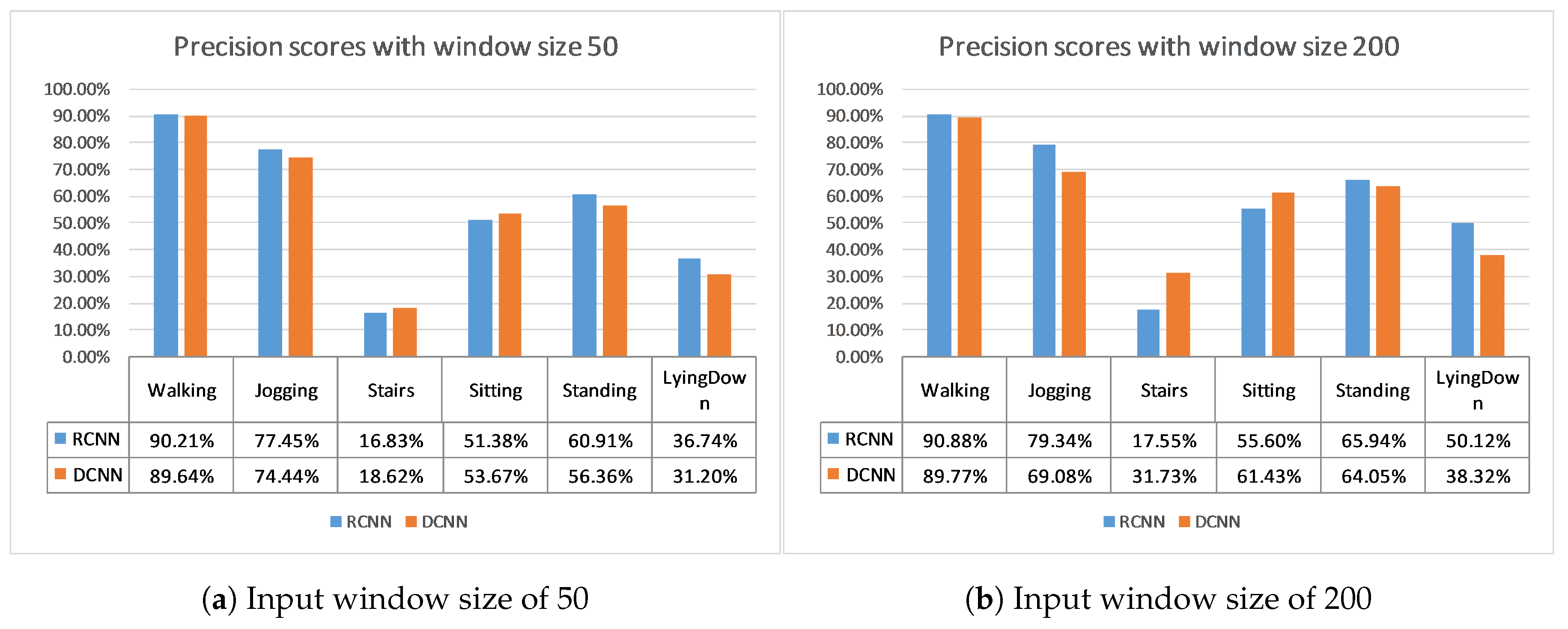
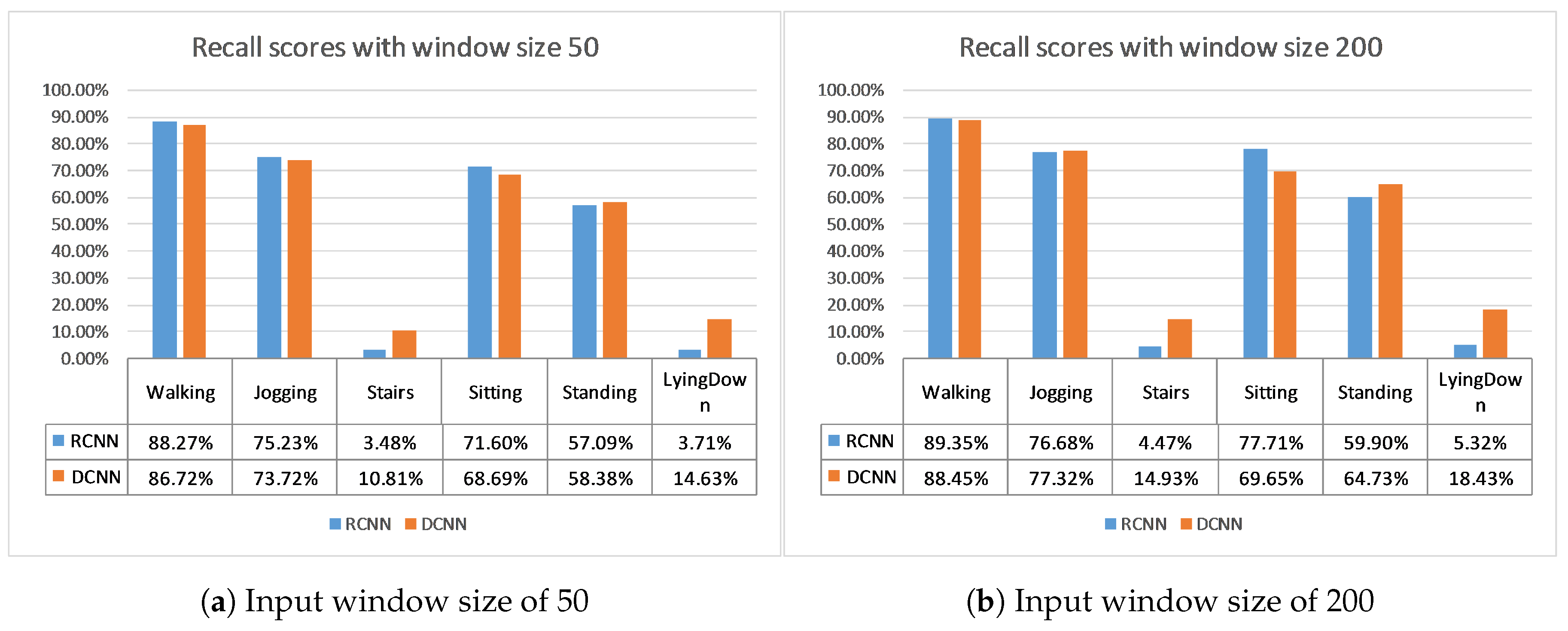
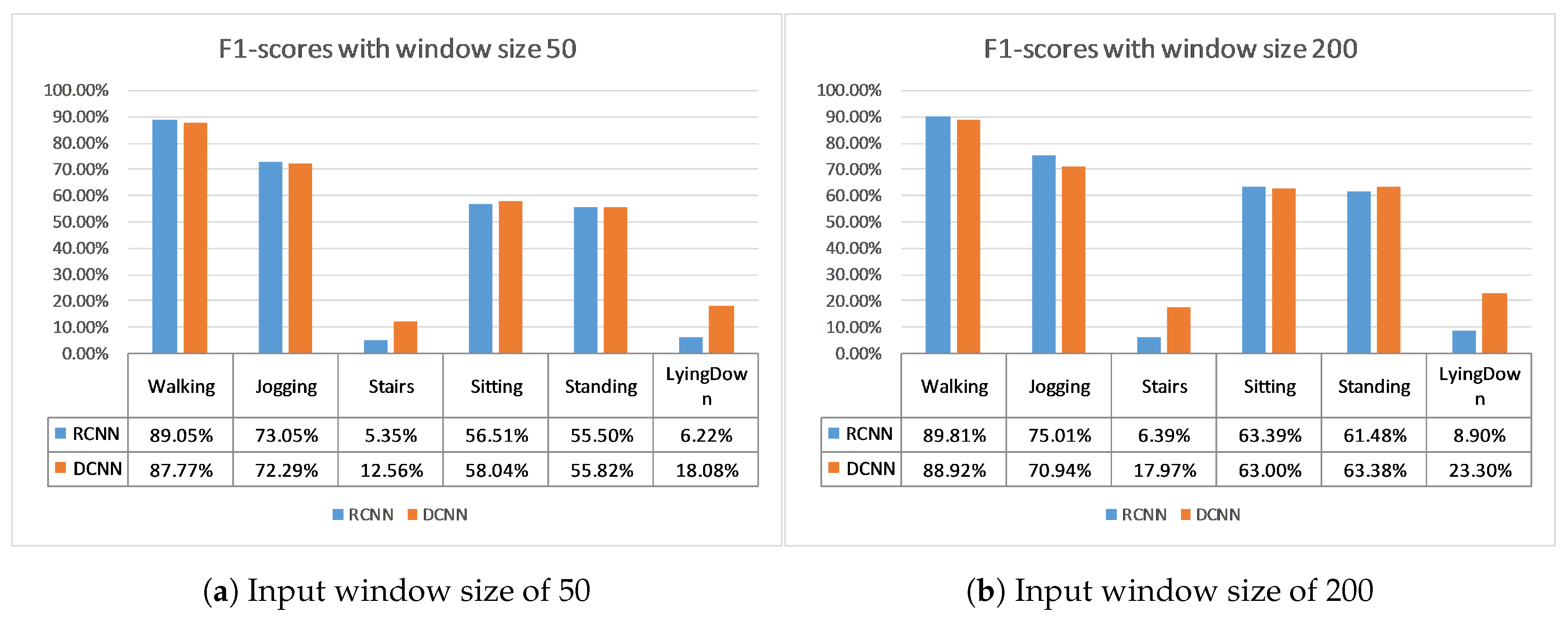
5. Discussion and Conclusions

When designing an implementation for mobile use, where the storage capacity is restricted, decreasing its size is a main goal. The size of a model depends on the number of its parameters, so it is the first variable that must be analyzed. We will provide an analysis for the variation of the model with an input size of 200 in favor of conciseness, but the results are similar for the one with an input size of 50. It is clear in

Table 15. Parameters per layer of the convolutional neural networks.

	DCNN	RCNN
Convolutional Layer 1	0.007 M	0.009 M
Convolutional Layer 2	0.22 M	-
Fully-connected layer	1.15 M	10.08 M
Softmax layer	0.003 M	0.006 M
Total	1.38 M	10.095 M

that the fully-connected layer is the one that contains the bulk of the model’s parameters. The proposed model has almost ten times less parameters than the original one, which is due to two factors. The layer has half as many nodes as the original, and the addition of the second convolutional layer further decreases the size of the input to this layer. This convolutional layer does contribute additional parameters to the network, but this increase is negligible compared to the decrease in the fully-connected layer. This explains the considerably smaller model size of the proposed network. The smaller model size combined with the faster inference time makes the DCNN model a better fit for real-time mobile implementations.

Furthermore, the smaller and more efficient design not only does not decrease the prediction performance, but consistently slightly increases it, achieving state-of-the-art performance amongst subject-independent implementations. It is considered important to note here the motivation behind choosing and comparing against only subject-independent solutions. The main goal is to correctly evaluate the generalization capability of the network, since “seeing” data points of a subject in the training set can help the inference of the same subject in the test set, and there is no guarantee that this will work as effectively for a subject that was never in the training set [66]. Moreover, targeting a real-time mobile use case means that the training will be performed on a desktop and the model will be used on a mobile device for inference. In most cases, the dataset for training the model will not contain data points of the end user, especially if the application becomes publicly available. Finally, the comparison of the results of subject-independent and subject-dependent solutions is unfair, since the scores of the subject-dependent solutions are expected to be higher.

Statistical feature analysis is also performed to evaluate the importance of the features and the possible alternative approaches. More specifically, the results indicate clearly that the use of the 40 statistical features improves the performance of the network, and at the same time, all of the different feature types contribute, albeit with varying impact, to this improvement. Using PCA would help decrease the dimensionality of the feature input, but in our case, it results in inferior performance, instead. The main reason is that it requires normalization, in order to properly estimate the variance of each feature, and thus, it distorts the scale of these features. This is supported by the fact that using no features at all achieves higher performance than using normalized features.

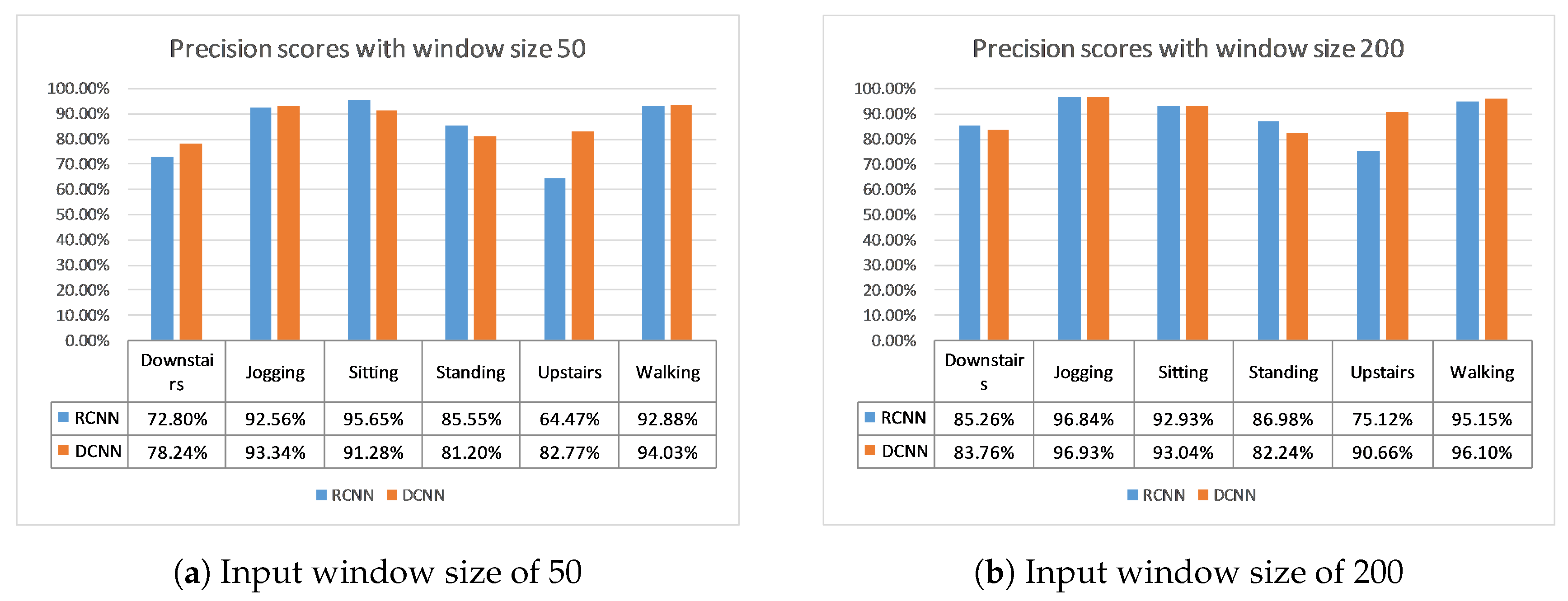
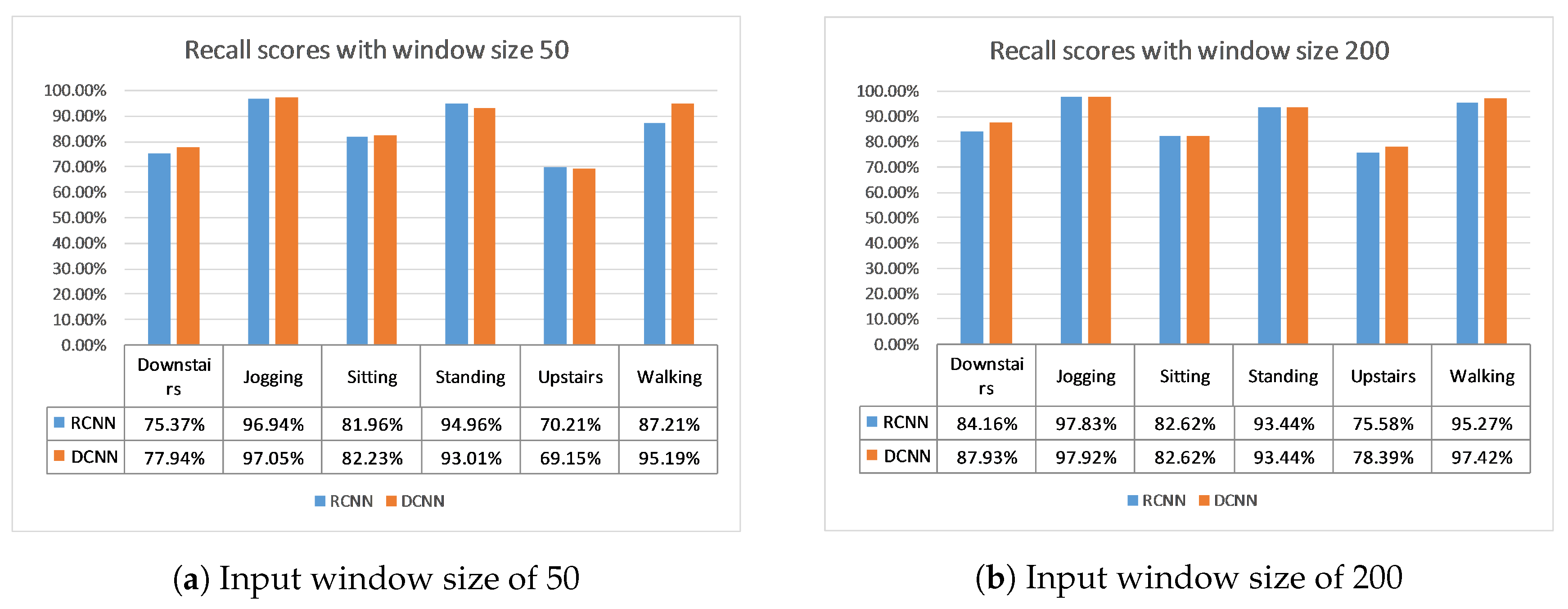
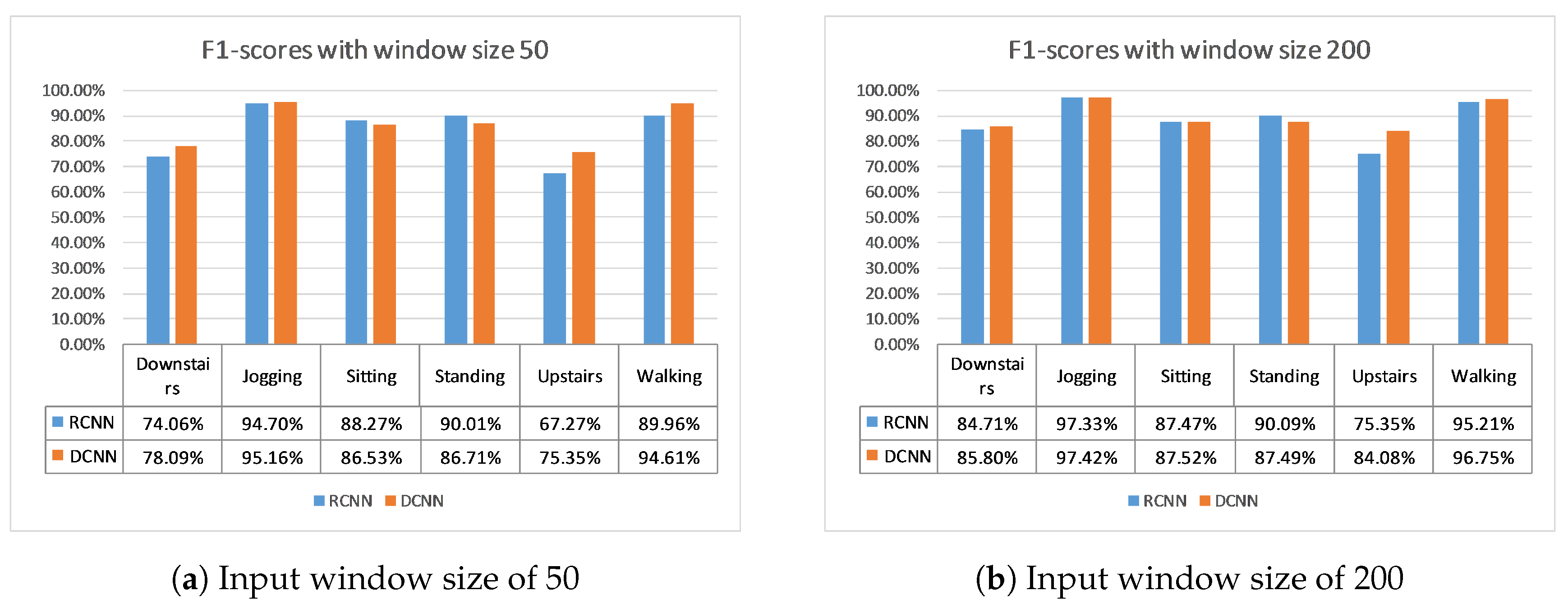
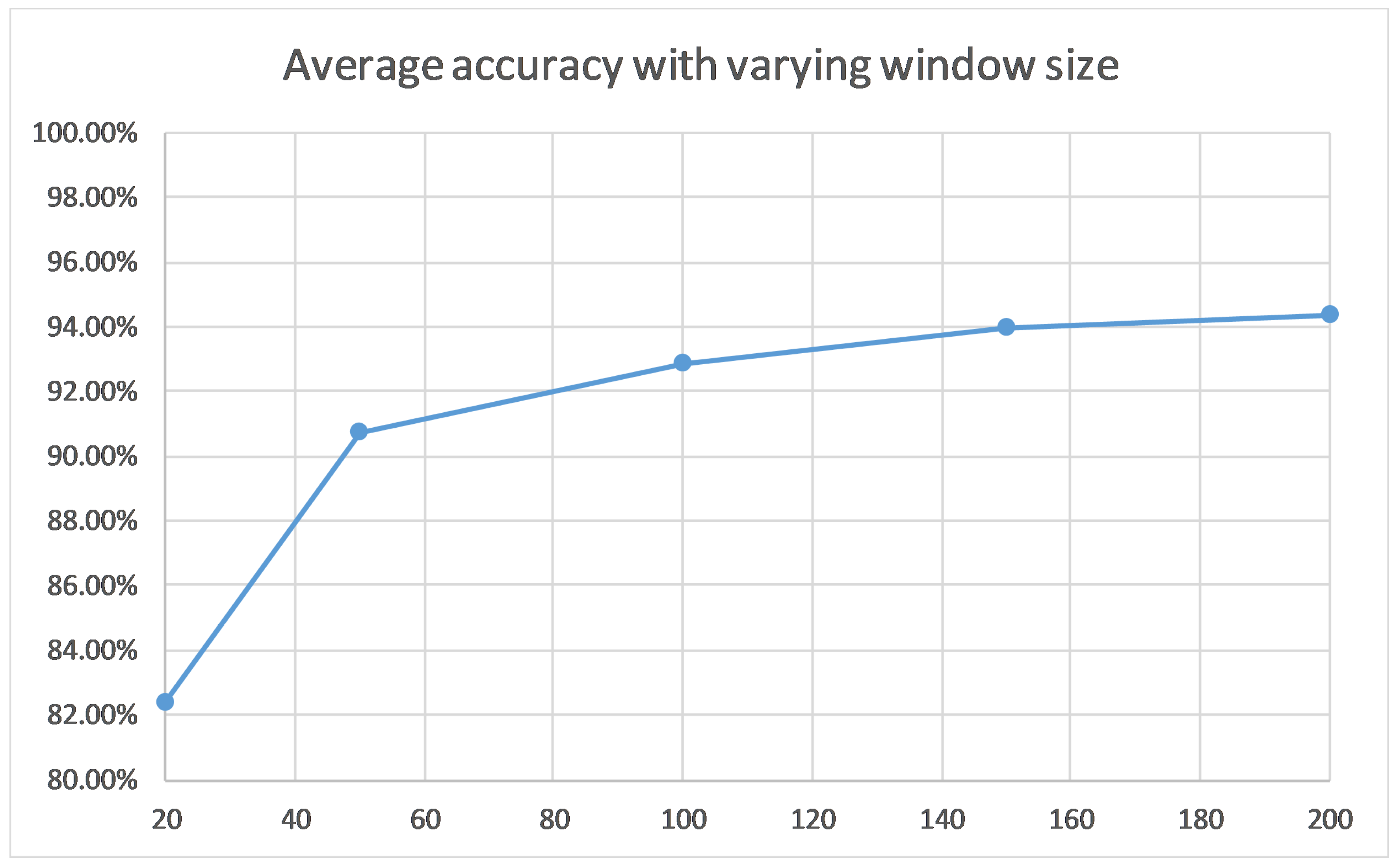
Finally, a window size analysis will enable each implementation of our solution to select the window size that more closely fits their specifications. It also justifies the selection of window size of 50 for a good trade-off of performance and efficiency and the selection of window size of 200 as the best performing one, if speed is not the most important factor.

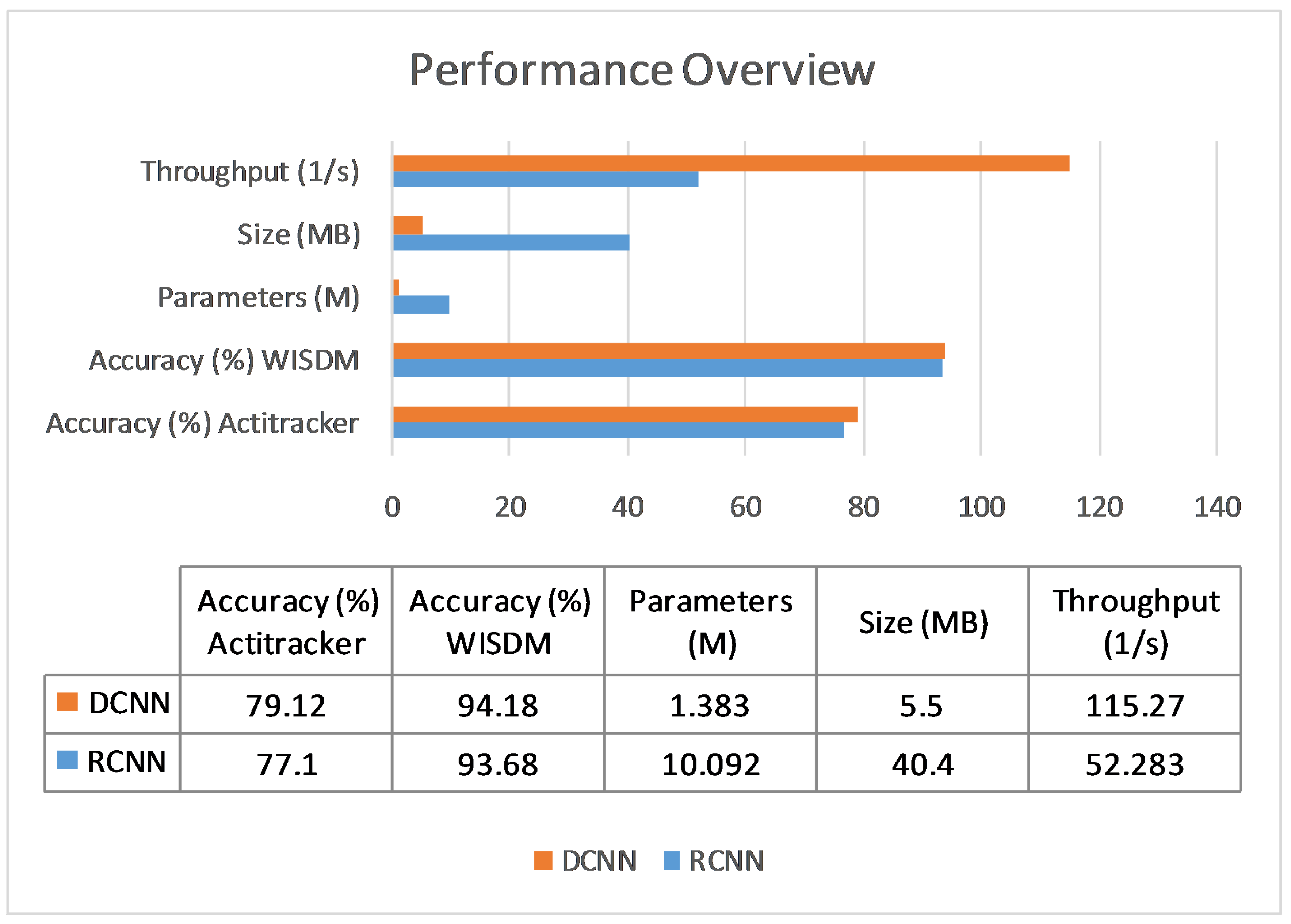
In conclusion, a novel model to recognize physical activities using only the accelerometer data from a mobile device in real time is proposed. It improves upon the state-of-the-art solution by employing a deeper convolutional neural network structure and changing the optimization methods. This improvement is evident at many levels. Firstly, the number of parameters and the size of the model are five to eight times smaller than the previous state-of-the-art model, for instance 1.383 million model parameters instead of 10.092 million for a window size of 200. The throughput is also improved, since it is two to three times higher, namely 405 inferences per second compared to 206.88 of the previous state-of-the-art and a window size of 50. Moreover, the classification performance is better and more robust, since both models are tested on two datasets and 10-fold cross-validation is also used. Indicatively, the average accuracy on the 10-fold cross-validation on the WISDM and Actitracker datasets for a window size of 200 is 94.18% and 79.12%, 0.5% and 2% higher than the previous state-of-the-art. This means that this solution is better in terms of size, throughput, and performance, all of which are crucial for a real-time on-device application, as can be seen in Figure 9. As an additional contribution, we investigated the impact of the statistical features in order to validate their importance and offer a comparison between the 40 statistical features and the ones created using PCA.

Among the various limitations acknowledged in this work, certain factors have been identified as fields of further research to be pursued towards improving the results of the proposed system. Even deeper convolutional neural network structures can be explored, but the size of the network needs to always be in check. A probable solution would be to also use $1\times 1$ convolutions. Another convolutional neural network with a higher receptive field could also be an alternative for substituting the global features. Finally, an implementation that also uses the gyroscope data would be interesting.

References

1. Oguntala, G.A.; Abd-Alhameed, R.A.; Ali, N.T.; Hu, Y.; Noras, J.M.; Eya, N.N.; Elfergani, I.; Rodriguez, J. SmartWall: Novel RFID-Enabled Ambient Human Activity Recognition Using Machine Learning for Unobtrusive Health Monitoring. IEEE Access 2019, 7, 68022–68033. [Google Scholar] [CrossRef]
2. Wang, F.; Gong, W.; Liu, J.; Wu, K. Channel Selective Activity Recognition with WiFi: A Deep Learning Approach Exploring Wideband Information. IEEE Trans. Netw. Sci. Eng. 2018, 7, 181–192. [Google Scholar] [CrossRef]
3. Cao, L.; Wang, Y.; Zhang, B.; Jin, Q.; Vasilakos, A.V. GCHAR: An efficient Group-based Context-aware human activity recognition on smartphone. J. Parallel Distrib. Comput. 2018, 118, 67–80. [Google Scholar] [CrossRef]
4. Zhang, L.; Wu, X.; Luo, D. Improving activity recognition with context information. In Proceedings of the 2015 IEEE International Conference on Mechatronics and Automation (ICMA), Beijing, China, 2–5 August 2015; pp. 1241–1246. [Google Scholar] [CrossRef]
5. Gao, Z.; Liu, D.; Huang, K.; Huang, Y. Context-Aware Human Activity and Smartphone Position-Mining with Motion Sensors. Remote Sens. 2019, 11, 2531. [Google Scholar] [CrossRef] [Green Version]
6. Hsu, Y.; Yang, S.; Chang, H.; Lai, H. Human Daily and Sport Activity Recognition Using a Wearable Inertial Sensor Network. IEEE Access 2018, 6, 31715–31728. [Google Scholar] [CrossRef]
7. Hsu, Y.; Chang, H.; Chiu, Y. Wearable Sport Activity Classification Based on Deep Convolutional Neural Network. IEEE Access 2019, 7, 170199–170212. [Google Scholar] [CrossRef]
8. Yang, S.; Gao, B.; Jiang, L.; Jin, J.; Gao, Z.; Ma, X.; Woo, W.L. IoT Structured Long-Term Wearable Social Sensing for Mental Wellbeing. IEEE Internet Things J. 2019, 6, 3652–3662. [Google Scholar] [CrossRef]
9. Demrozi, F.; Bacchin, R.; Tamburin, S.; Cristani, M.; Pravadelli, G. Toward a Wearable System for Predicting Freezing of Gait in People Affected by Parkinson’s Disease. IEEE J. Biomed. Health Inform. 2020, 24, 2444–2451. [Google Scholar] [CrossRef]
10. Chen, X.; Xue, H.; Kim, M.; Wang, C.; Youn, H.Y. Detection of Falls with Smartphone Using Machine Learning Technique. In Proceedings of the 2019 8th International Congress on Advanced Applied Informatics (IIAI-AAI), Toyama, Japan, 7–11 July 2019; pp. 611–616. [Google Scholar] [CrossRef]
11. Li, M.; O’Grady, M.; Gu, X.; Alawlaqi, M.A.; O’Hare, G. Time-bounded Activity Recognition for Ambient Assisted Living. IEEE Trans. Emerg. Top. Comput. 2018. [Google Scholar] [CrossRef]
12. Cook, D.; Schmitter-Edgecombe, M. Assessing the quality of activities in a smart environment. Methods Inf. Med. 2009, 48, 480–485. [Google Scholar]
13. Wang, Q.; Timmermans, A.; Chen, W.; Jia, J.; Ding, L.; Xiong, L.; Rong, J.; Markopoulos, P. Stroke Patients’ Acceptance of a Smart Garment for Supporting Upper Extremity Rehabilitation. IEEE J. Transl. Eng. Health Med. 2018, 6, 2101009. [Google Scholar] [CrossRef] [PubMed]
14. United Nations. World Population Prospects 2019: Highlights; United Nations Department for Economic and Social Affairs: New York, NY, USA, 2019. [Google Scholar]
15. Wang, J.; Chen, Y.; Hao, S.; Peng, X.; Lisha, H. Deep Learning for Sensor-based Activity Recognition: A Survey. Pattern Recognit. Lett. 2017, 119, 3–11. [Google Scholar] [CrossRef] [Green Version]
16. Goyal, R.; Kahou, S.E.; Michalski, V.; Materzynska, J.; Westphal, S.; Kim, H.; Haenel, V.; Fründ, I.; Yianilos, P.; Mueller-Freitag, M.; et al. The “something something” video database for learning and evaluating visual common sense. arXiv 2017, arXiv:1706.04261. [Google Scholar]
17. Fouhey, D.F.; Kuo, W.; Efros, A.A.; Malik, J. From Lifestyle Vlogs to Everyday Interactions. arXiv 2017, arXiv:1712.02310. [Google Scholar]
18. Damen, D.; Doughty, H.; Farinella, G.M.; Fidler, S.; Furnari, A.; Kazakos, E.; Moltisanti, D.; Munro, J.; Perrett, T.; Price, W.; et al. Scaling Egocentric Vision: The EPIC-KITCHENS Dataset. arXiv 2018, arXiv:1804.02748. [Google Scholar]
19. Banos, O.; Garcia, R.; Holgado-Terriza, J.A.; Damas, M.; Pomares, H.; Rojas, I.; Saez, A.; Villalonga, C. mHealthDroid: A Novel Framework for Agile Development of Mobile Health Applications. In Ambient Assisted Living and Daily Activities; Pecchia, L., Chen, L.L., Nugent, C., Bravo, J., Eds.; Springer International Publishing: Cham, Switzerland, 2014; pp. 91–98. [Google Scholar]
20. Banos, O.; Villalonga, C.; Garcia, R.; Saez, A.; Damas, M.; Holgado-Terriza, J.; Lee, S.; Pomares, H.; Rojas, I. Design, implementation and validation of a novel open framework for agile development of mobile health applications. Biomed. Eng. Online 2015, 14, S6. [Google Scholar] [CrossRef] [Green Version]
21. Chavarriaga, R.; Sagha, H.; Calatroni, A.; Digumarti, S.T.; Millan, J.d.R.; Roggen, D.; Tröster, G. The Opportunity challenge: A benchmark database for on-body sensor-based activity recognition. Pattern Recognit. Lett. 2013, 23, 2033–2042. [Google Scholar] [CrossRef] [Green Version]
22. Reiss, A.; Stricker, D. Introducing a New Benchmarked Dataset for Activity Monitoring. In Proceedings of the 2012 16th International Symposium on Wearable Computers, Newcastle, UK, 18–22 June 2012; pp. 108–109. [Google Scholar]
23. Zhang, M.; Sawchuk, A.A. USC-HAD: A Daily Activity Dataset for Ubiquitous Activity Recognition Using Wearable Sensors. In Proceedings of the ACM International Conference on Ubiquitous Computing (Ubicomp) Workshop on Situation, Activity and Goal Awareness (SAGAware), Pittsburgh, PA, USA, 5–8 September 2012; pp. 1036–1043. [Google Scholar] [CrossRef]
24. Chen, C.; Jafari, R.; Kehtarnavaz, N. UTD-MHAD: A multimodal dataset for human action recognition utilizing a depth camera and a wearable inertial sensor. In Proceedings of the 2015 IEEE International Conference on Image Processing (ICIP), Quebec City, QC, Canada, 27–30 September 2015; pp. 168–172. [Google Scholar] [CrossRef]
25. Bruno, B.; Mastrogiovanni, F.; Sgorbissa, A. Wearable Inertial Sensors: Applications, Challenges, and Public Test Benches. Robot. Autom. Mag. IEEE 2015, 22, 116–124. [Google Scholar] [CrossRef]
26. Kwapisz, J.R.; Weiss, G.M.; Moore, S.A. Activity Recognition Using Cell Phone Accelerometers. SIGKDD Explor. Newsl. 2011, 12, 74–82. [Google Scholar] [CrossRef]
27. Lockhart, J.W.; Weiss, G.M.; Xue, J.C.; Gallagher, S.T.; Grosner, A.B.; Pulickal, T.T. Design Considerations for the WISDM Smart Phone-based Sensor Mining Architecture. In Proceedings of the Fifth International Workshop on Knowledge Discovery from Sensor Data, San Diego, CA, USA, 21–24 August 2011; pp. 25–33. [Google Scholar] [CrossRef] [Green Version]
28. van Kasteren, T.L.M.; Englebienne, G.; Kröse, B.J.A. Human Activity Recognition from Wireless Sensor Network Data: Benchmark and Software. In Activity Recognition in Pervasive Intelligent Environments; Atlantis Press: Paris, France, 2011; pp. 165–186. [Google Scholar] [CrossRef]
29. Nweke, H.; Wah, T.; Al-Garadi, M.; Alo, U. Deep Learning Algorithms for Human Activity Recognition using Mobile and Wearable Sensor Networks: State of the Art and Research Challenges. Expert Syst. Appl. 2018, 105. [Google Scholar] [CrossRef]
30. Lara, O.D.; Labrador, M.A. A Survey on Human Activity Recognition using Wearable Sensors. IEEE Commun. Surv. Tutor. 2013, 15, 1192–1209. [Google Scholar] [CrossRef]
31. Bengio, Y. Deep Learning of Representations: Looking Forward. In Statistical Language and Speech Processing; Springer: Berlin/Heidelberg, Geramny, 2013; pp. 1–37. [Google Scholar]
32. Morales, J.; Akopian, D. Physical activity recognition by smartphones, a survey. Biocybern. Biomed. Eng. 2017, 37, 388–400. [Google Scholar] [CrossRef]
33. Salzberg, S.L. C4.5: Programs for Machine Learning by J. Ross Quinlan. Morgan Kaufmann Publishers, Inc., 1993. Mach. Learn. 1994, 16, 235–240. [Google Scholar] [CrossRef] [Green Version]
34. Kumar, A. Human Activity Recognition through Smartphone’s Tri-Axial Accelerometer using Time Domain Wave Analysis and Machine Learning. Int. J. Comput. Appl. 2015, 127, 22–26. [Google Scholar] [CrossRef]
35. Ignatov, A. Real-time human activity recognition from accelerometer data using Convolutional Neural Networks. Appl. Soft Comput. 2018, 62, 915–922. [Google Scholar] [CrossRef]
36. Tharwat, A.; Mahdi, H.; Elhoseny, M.; Hassanien, A.E. Recognizing human activity in mobile crowdsensing environment using optimized k-NN algorithm. Expert Syst. Appl. 2018, 107, 32–44. [Google Scholar] [CrossRef]
37. Anguita, D.; Ghio, A.; Oneto, L.; Parra, X.; Reyes-Ortiz, J.L. Human activity recognition on smartphones using a multiclass hardware-friendly support vector machine. In Proceedings of the International Workshop on Ambient Assisted Living, Vitoria-Gasteiz, Spain, 3–5 December 2012; pp. 216–223. [Google Scholar]
38. Lara, O.D.; Pérez, A.J.; Labrador, M.A.; Posada, J.D. Centinela: A human activity recognition system based on acceleration and vital sign data. Pervasive Mob. Comput. 2012, 8, 717–729. [Google Scholar] [CrossRef]
39. Hammerla, N.Y.; Halloran, S.; Ploetz, T. Deep, Convolutional, and Recurrent Models for Human Activity Recognition Using Wearables. arXiv 2016, arXiv:1604.08880. [Google Scholar]
40. Ordonez, F.J.; Roggen, D. Deep Convolutional and LSTM Recurrent Neural Networks for Multimodal Wearable Activity Recognition. Sensors 2016, 16, 115. [Google Scholar] [CrossRef] [Green Version]
41. Stiefmeier, T.; Roggen, D.; Ogris, G.; Lukowicz, P.; Tröster, G. Wearable Activity Tracking in Car Manufacturing. IEEE Pervasive Comput. 2008, 7, 42–50. [Google Scholar] [CrossRef]
42. Anguita, D.; Ghio, A.; Oneto, L.; Parra, X.; Reyes-Ortiz, J.L. A Public Domain Dataset for Human Activity Recognition Using Smartphones. In Proceedings of the 21st European Symposium on Artificial Neural Networks, ESANN 2013, Bruges, Belgium, 24–26 April 2013. [Google Scholar]
43. Sikder, N.; Chowdhury, M.; Arif, A.; Nahid, A. Human Activity Recognition Using Multichannel Convolutional Neural Network. In Proceedings of the 2019 5th International Conference on Advances in Electrical Engineering (ICAEE), Dhaka, Bangladesh, 26–28 September 2019. [Google Scholar]
44. Ronao, C.A.; Cho, S.B. Human activity recognition with smartphone sensors using deep learning neural networks. Expert Syst. Appl. 2016, 59, 235–244. [Google Scholar] [CrossRef]
45. Kolosnjaji, B.; Eckert, C. Neural network-based user-independent physical activity recognition for mobile devices. In Proceedings of the IDEAL 2015: 16th International Conference, Wroclaw, Poland, 14–16 October 2015; pp. 378–386. [Google Scholar]
46. Huang, J.; Lin, S.; Wang, N.; Dai, G.; Xie, Y.; Zhou, J. TSE-CNN: A Two-Stage End-to-End CNN for Human Activity Recognition. IEEE J. Biomed. Health Inform. 2020, 24, 292–299. [Google Scholar] [CrossRef] [PubMed]
47. Alsheikh, M.A.; Selim, A.; Niyato, D.; Doyle, L.; Lin, S.; Tan, H.P. Deep Activity Recognition Models with Triaxial Accelerometers. arXiv 2016, arXiv:1511.04664. [Google Scholar]
48. Milenkoski, M.; Trivodaliev, K.; Kalajdziski, S.; Jovanov, M.; Stojkoska, B.R. Real time human activity recognition on smartphones using LSTM networks. In Proceedings of the 2018 41st International Convention on Information and Communication Technology, Electronics and Microelectronics (MIPRO), Opatija, Croatia, 21–25 May 2018; pp. 1126–1131. [Google Scholar]
49. Pienaar, S.W.; Malekian, R. Human Activity Recognition using LSTM-RNN Deep Neural Network Architecture. In Proceedings of the 2019 IEEE 2nd Wireless Africa Conference (WAC), Pretoria, South Africa, 18–20 August 2019; pp. 1–5. [Google Scholar] [CrossRef] [Green Version]
50. Wang, X.; Liao, W.; Guo, Y.; Yu, L.; Wang, Q.; Pan, M.; Li, P. PerRNN: Personalized Recurrent Neural Networks for Acceleration-Based Human Activity Recognition. In Proceedings of the ICC 2019—2019 IEEE International Conference on Communications (ICC), Shanghai, China, 20–24 May 2019; pp. 1–6. [Google Scholar] [CrossRef]
51. Chen, Y.; Zhong, K.; Zhang, J.; Sun, Q.; Zhao, X. LSTM Networks for Mobile Human Activity Recognition. In Proceedings of the 2016 International Conference on Artificial Intelligence: Technologies and Applications, Bangkok, Thailand, 24–25 January 2016. [Google Scholar] [CrossRef] [Green Version]
52. Xu, W.; Pang, Y.; Yang, Y.; Liu, Y. Human Activity Recognition Based On Convolutional Neural Network. In Proceedings of the 2018 24th International Conference on Pattern Recognition (ICPR), Beijing, China, 20–24 August 2018; pp. 165–170. [Google Scholar] [CrossRef]
53. Zeng, M.; Nguyen, L.T.; Yu, B.; Mengshoel, O.J.; Zhu, J.; Wu, P.; Zhang, J. Convolutional neural networks for human activity recognition using mobile sensors. In Proceedings of the 6th International Conference on Mobile Computing, Applications and Services, Austin, TX, USA, 6–7 November 2014; pp. 197–205. [Google Scholar]
54. Alsheikh, M.A.; Niyato, D.; Lin, S.; Tan, H.; Han, Z. Mobile big data analytics using deep learning and apache spark. IEEE Netw. 2016, 30, 22–29. [Google Scholar] [CrossRef] [Green Version]
55. Shakya, S.; Zhang, C.; Zhou, Z. Comparative Study of Machine Learning and Deep Learning Architecture for Human Activity Recognition Using Accelerometer Data. Int. J. Mach. Learn. Comput. 2018, 8, 577–582. [Google Scholar]
56. Ravì, D.; Wong, C.; Lo, B.; Yang, G.Z. A Deep Learning Approach to on-Node Sensor Data Analytics for Mobile or Wearable Devices. IEEE J. Biomed. Health Inform. 2016. [Google Scholar] [CrossRef] [Green Version]
57. Ravi, D.; Wong, C.; Lo, B.; Yang, G. Deep learning for human activity recognition: A resource efficient implementation on low-power devices. In Proceedings of the 2016 IEEE 13th International Conference on Wearable and Implantable Body Sensor Networks (BSN), San Francisco, CA, USA, 14–17 June 2016; pp. 71–76. [Google Scholar] [CrossRef] [Green Version]
58. Yazdanbakhsh, O.; Dick, S. Multivariate Time Series Classification using Dilated Convolutional Neural Network. arXiv 2019, arXiv:1905.01697. [Google Scholar]
59. Siirtola, P.; Röning, J. Recognizing Human Activities User-independently on Smartphones Based on Accelerometer Data. Int. J. Interact. Multimed. Artif. Intell. 2012, 1, 38–45. [Google Scholar] [CrossRef]
60. Antonsson, E.K.; Mann, R.W. The frequency content of gait. J. Biomech. 1985, 18, 39–47. [Google Scholar] [CrossRef]
61. De La Concepción, M.Á.; Morillo, L.S.; Gonzalez-Abril, L.; Ramírez, J.O. Discrete techniques applied to low-energy mobile human activity recognition. A new approach. Expert Syst. Appl. 2014, 41, 6138–6146. [Google Scholar] [CrossRef] [Green Version]
62. Nair, V.; Hinton, G.E. Rectified Linear Units Improve Restricted Boltzmann Machines. In Proceedings of the ICML, Haifa, Israel, 21–24 June 2010. [Google Scholar]
63. Yamaguchi, K.; Sakamoto, K.; Akabane, T.; Fujimoto, Y. A neural network for speaker-independent isolated word recognition. In Proceedings of the ICSLP-1990, Kobe, Japan, 18–22 November 1990; pp. 1077–1080. [Google Scholar]
64. Robbins, H.; Monro, S. A Stochastic Approximation Method. Ann. Math. Stat. 1951, 22, 400–407. [Google Scholar] [CrossRef]
65. Qian, N. On the momentum term in gradient descent learning algorithms. Neural Netw. Off. J. Int. Neural Netw. Soc. 1999, 12, 145–151. [Google Scholar] [CrossRef]
66. Micucci, D.; Mobilio, M.; Napoletano, P. UniMiB SHAR: A new dataset for human activity recognition using acceleration data from smartphones. Appl. Sci. 2017, 7, 1101. [Google Scholar] [CrossRef] [Green Version]
Figure 1. Detailed network architecture.
Applsci 10 08482 g001
Figure 2. Precision scores on the original train/test split of the WISDM dataset.
Applsci 10 08482 g002
Figure 3. Recall scores on the original train/test split of the WISDM dataset.
Applsci 10 08482 g003
Figure 4. F1-scores on the original train/test split of the WISDM dataset.
Applsci 10 08482 g004
Figure 5. Average precision scores of the 10-fold cross-validation of the Actitracker dataset.
Applsci 10 08482 g005
Figure 6. Average recall scores of the 10-fold cross-validation of the Actitracker dataset.
Applsci 10 08482 g006
Figure 7. Average f1-scores of the 10-fold cross-validation of the Actitracker dataset.
Applsci 10 08482 g007
Figure 8. Average accuracy of the original train/test split of the WISDM dataset for varying window sizes.
Applsci 10 08482 g008
Figure 9. Overview of the performance of the proposed model. It is noted that in the accuracy and throughput categories, the higher the better, while the inverse holds for the size and the number of parameters.
Applsci 10 08482 g009