Numerical Analysis of a Single-Stage Fast Linear Transformer Driver Using Field-Circuit Coupled Time-Domain Finite Integration Theory

Abstract

The focus of this paper is numerical analysis on the performance of a newly designed mega-ampere (MA) class single-stage fast linear transformer driver (FLTD) with 24 separate columns in the China Z-pinch driver CZ34. However, the internal structure and media distribution of the FLTD induction cavity is very complicated and the short rise time of the bricks’ discharge current will make spatial discretization much denser, resulting in a dramatic increase in the computational complexity of a 3-D model. In this paper, the electromagnetic (EM) characteristics of the single-stage FLTD with 24-separate columns are investigated based on the time-domain finite integration theory (TD-FIT). The discharge currents of brick capacitors in the circuit model are coupled to the field model as excitations. The grid size of the key components in FLTD cavity are refined by nonuniform grids. To further reduce the number of degrees of freedom (DoFs), the surface impedance boundary condition (SIBC) is used to model good conductors. Measurements and simulation results demonstrate that TD-FIT is effective and accurate in analyzing the EM transients of FLTD. Equivalent inductance of the discharging brick will increase by ~35 nH due to the mutual flux linkage among neighboring bricks when all the 23-bricks are triggered synchronously.

1. Introduction

Controlled nuclear fusion energy is the ideal clean and safe energy for the future. To realize controlled nuclear fusion, technologies such as magnetic confinement fusion (e.g., Tokamak, stellarator, and reversed-field pinch (RFP) [1]) and inertial confinement fusion (e.g., Z-pinch and laser fusion [2]) have been developed. Compared with Tokamak, Z-pinch is more cost-effective. In addition, Z-pinch has a shorter load current rise time and higher repetition rate than that of RFP. A Z-pinch (or zeta pinch) machine creates an azimuthal magnetic field when an axial (along the zeta-axis in a cylindrical coordinate system) current flows through the electrically conducting filament [2]. The fast Z-pinch needs very high energy densities with rise time of load current less than 100 ns [2]. It plays a very important role in the fields of intense radiation effect, high energy density physics, inertial confinement fusion, inertial fusion energy, material science under extreme conditions, and laboratory astrophysics [3,4,5], to name a few. Traditionally, a Z-pinch pulsed power driver is based on the μs-class Marx-generator and pulse-forming technology. However, Marx-architecture has drawbacks such as low energy transfer efficiency, low repetition rate, and high components withstand voltage [3]. The fast linear transformer driver (FLTD) has been developed for the last 20 years which can directly generate high power pulses with rise time less than 100-ns and amplitude up to 1-MA [4]. FLTD is generally considered to be one of the most promising technologies for the next generation Z-pinch driver.

In FLTD configuration, the basic building block is called “brick”, which is composed of two film capacitors and one low-inductance gas switch connected in series. In essence, a brick is a single-stage Marx generator and can be regarded as a series-connected RLC circuit. Dozens of discharging bricks are arranged azimuthally around magnetic cores in the primary side of the FLTD cavity and are connected in parallel to a coaxial water-insulated transmission line impedance transformer in the secondary side of the FLTD cavity. To achieve synchronous triggering of bricks in the same cavity and sequential triggering of bricks in different cavities, tens of thousands of trigger signals are required in an FLTD based pulsed-power accelerator, leading to immensely complicated charging- and triggering-systems. Sun et al. [6] proposed a triggering scheme based on a triggering brick and azimuthal transmission line inside the FLTD cavity, reducing complexity of the triggering system. As depicted in Figure 1, in each stage, there are 23 discharging bricks and one triggering brick packaged in the proposed FLTD cavity. Figure 2 illustrates cross sectional view of the FLTD cavity. The discharging bricks are connected to the stainless-steel cavity via the mounting brackets (items J and K in Figure 2). To improve maintainability, the cavity outer cylindrical wall in a traditional FLTD is replaced with 24-separate columns (item Q in Figure 2). Based on this triggering technique, the 4-stage series-connected FLTD with sharing common cavity shell was presented in [7].

During the design and prototyping of FLTD, it is necessary to investigate self-consistent electromagnetic (EM) fields by using numerical approaches. FLTD and Z-pinch related simulations are usually performed with equivalent circuit model [8,9,10,11,12], finite-difference time-domain (FDTD) method [13,14,15], finite element method (FEM) [16,17,18,19,20], and partial element equivalent circuit (PEEC) method [21,22,23], etc. Koval’chuk et al. [8] proposed the concept of linear transformer driver (LTD) as a fast primary energy storage device for the first time and validated its output performance. Guo et al. [9] presented a 2-D circuit model for simulating power flow of the induction cavity. Liu et al. [10] investigated the influence of switching jitter on the output current of a 60-cavities LTD module based on the whole circuit model. Zhang et al. [11] developed the concept of hybrid mode LTD stage and analyzed its output current with a circuit model. Zhou el al. [12] established a whole circuit model for the Z-800 machine and obtained the optimal load parameters. The equivalent circuit model is very efficient for the analysis of electrical performance, but it is impossible to describe detailed field distribution inside FLTD induction cavity. Rose et al. [13] established a 3-D model of the 1-MA LTD cavities using the LSP Suite software. They calculated generation and propagation of electromagnetic wave in LTD stage. Wei et al. [14] compared effects of two different dielectric media in induction cavity on the operational performance using the FDTD algorithm. In [15], Wei et al. studied azimuthal uniformity of injection currents in induction cavity based on 3-D electromagnetic numerical model. FDTD method is simple in terms of implementation and programming and it can effectively deal with EM wave propagation problems [24]. However, its calculation accuracy is limited by the staircase approximation of the Yee-cell and numerical dispersion. Reisman et al. [16] used iterative FEM, circuit, and magneto-hydro-dynamic (MHD) simulations to determine the design of a pulsed power accelerator. Bettini et al. [17] calculated static halo currents in magnetic confinement fusion devices based on electric vector potential and geometric mixed-hybrid formulations of finite element. Yanovskiy et al. [18] addressed the poloidal distributions of EM load in the vacuum vessel of COMPASS-U tokamak with ANSYS Maxwell and CarMa0NL. Gourdain et al. [19] analyzed geometries of nested transmission lines in the FLTD driven accelerator using the RF module of FEM software COMSOL. Flisgen et al. [20] implemented frequency domain higher-order FEM to determine the generalized scattering matrices of a long accelerator structure. FEM is suitable for modeling complex structures and media distributions [25]; nevertheless, it has low calculation speed and high memory consumption [26]. Yan et al. [21] investigated and optimized the output current of a multi-brick parallel discharge driver using the PEEC method. Voltolina et al. [22] coupled low rank approximation with the PEEC equations for efficient modeling of thermonuclear fusion facility. Abate et al. [23] proposed fast and parallel modeling of the RFX-mod fusion machine with integral equation method and hybrid CPU-GPU parallelization. The PEEC method can directly embed transient EM model of the multi-conductor system into circuit model [27], but it is difficult to model materials with intricate distribution [28].

The finite integration theory (FIT) is proposed by Weiland [29] and then it is combined with particle-in-cell algorithm for simulating particle accelerators [30,31,32]. FIT starts with Maxwell’s equations in integral form and defines integration of field quantity on the edge or facet of a grid as degree of freedom (DoF) [31]. Unlike differential variables, integral variables can be directly measured by experiments and are continuous through the separation surface of different materials. FIT is a spatial discretization strategy to numerically solve EM field problems and can yield results in both time- and spectral-domain [32]. Schöps et al. [33] derived the field-circuit coupled formulations for time-domain FIT (TD-FIT) based on the concept of winding functions. Udosen et al. [34] used the FIT for simulating electrical resistivity tomography and verified its ability for large-scale computation. Razi-Kazemi et al. [35], Mao et al. [36], and Qiu et al. [37] employed CST Studio Suite to investigate applicability of the FIT for performance analysis of grounding system against high frequency waveforms, monolithic radial transmission line in a Z-pinch driver, and the single-stage FLTD cavity, respectively.

In this paper, based on our previous research in [6,37], EM characteristics of the MA-class single-stage FLTD with 24-separate columns are studied by using field-circuit coupled TD-FIT. The desired single-stage FLTD should have one triggering cable and load current of 1-MA amplitude and 100-ns rise time. In Section 2, basics of the TD-FIT are introduced. Construction of the FLTD cavity’s numerical model, especially the main discharging brick and magnetic core, is discussed at length in Section 3. To further improve calculation speed and reduce memory consumption, the nonuniform grid and first-order surface impedance boundary condition (SIBC) are employed. Performance of the single discharging brick, 23 discharging bricks, and sing-stage FLTD are investigated in Section 4. Concluding remarks are given in Section 5.

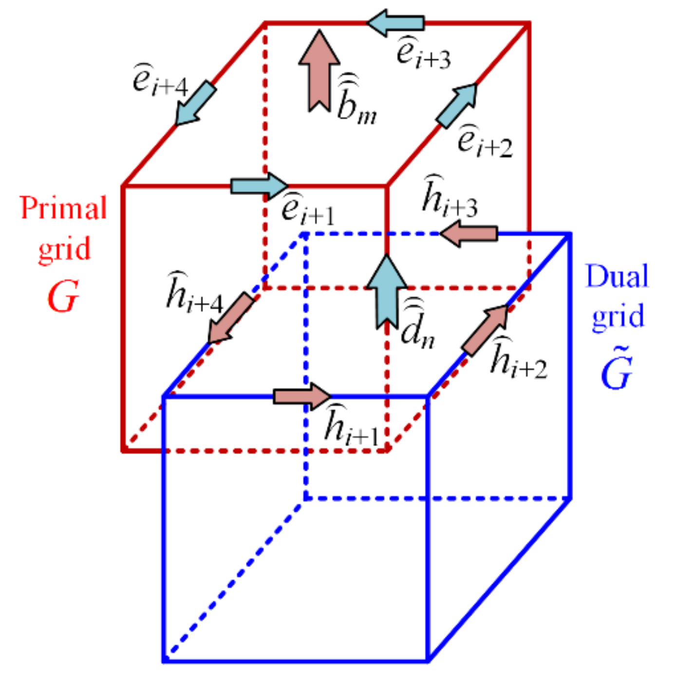
2. Time-Domain Finite Integration Theory (TD-FIT)

Similar to the Yee-cell of FDTD method, in FIT, discretized electric field components are allocated along the edges of primal grid $G$ while discretized magnetic field components are allocated along the edges of dual grid $\tilde{G}$. The hexahedral, orthogonal primal-dual grid pairs are staggered with each other by half a lattice length, as shown in Figure 3.

2.1. Definition of State Variables

In FIT, DoF is defined along the edge or through the facet of a grid, where the integral of grid edge is called voltage and integral of grid facet is called flux [31]:

$${\stackrel{⌢}{e}}_i={\displaystyle {\int }_{L_i}\mathit{E}\cdot d\mathit{s}},{\stackrel{⌢}{\stackrel{⌢}{b}}}_k={\displaystyle {\int }_{A_k}\mathit{B}\cdot d\mathit{A}},$$

(1)

$${\stackrel{⌢}{h}}_k={\displaystyle {\int }_{{\tilde{L}}_k}\mathit{H}\cdot d\mathit{s}},{\stackrel{⌢}{\stackrel{⌢}{d}}}_i={\displaystyle {\int }_{{\tilde{A}}_i}\mathit{D}\cdot d\mathit{A}},{\stackrel{⌢}{\stackrel{⌢}{i}}}_i={\displaystyle {\int }_{{\tilde{A}}_i}\mathit{J}\cdot d\mathit{A}},$$

(2)

where ${\stackrel{⌢}{e}}_i$ and ${\stackrel{⌢}{\stackrel{⌢}{b}}}_k$ denote electric voltage along the edge and magnetic flux through the facet of primal grid, respectively; ${\stackrel{⌢}{h}}_k$, ${\stackrel{⌢}{\stackrel{⌢}{d}}}_i$, and ${\stackrel{⌢}{\stackrel{⌢}{i}}}_i$ denote magnetic voltage along the edge, electric flux through the facet, and electric current through the facet of dual grid, respectively; $L_i$ is the i-th edge of primal grid, ${\tilde{A}}_i$ is the i-th facet of dual grid, $A_k$ is the k-th facet of primal grid, and ${\tilde{L}}_k$ is the k-th edge of dual grid.

2.2. Construction of Discrete Divergence and Curl Operator

In three-dimensional Cartesian coordinate system, the primal grid $G$ can be defined as:

$$\begin{array}{l}G=\left\{\left(x_i,y_j,z_k\right)\in R^3;\right.\\ \left.x_1\le x_i\le x_I,i=1,2,\dots ,I;y_1\le y_j\le y_J,j=1,2,\dots ,J;z_1\le z_k\le z_K,k=1,2,\dots ,K\right\},\end{array}$$

(3)

where I, J, and K denote the number of nodes along the x-, y-, and z-axis, respectively.

All the nodes of $G$ are numbered linearly in ascending order along the x-, y-, and z-axis:

$$n=1+\left(i-1\right)\cdot M_x+\left(j-1\right)\cdot M_y+\left(k-1\right)\cdot M_z,$$

(4)

where n denotes the present node number, $n=1,2,\dots ,N$; N denotes the total number of nodes of primal grid, $N=IJK$; $M_x=1$, $M_y=I$, $M_z=IJ$.

Then, we need to introduce three basic topological matrices of dimensions $N\times N$ to represent discrete partial differential operators with central difference approximation:

$$\frac{\partial }{\partial x}\iff P_x={\left(P_x\right)}_{m,n}=\left\{\begin{array}{l}-1n=m\\ 1n=m+M_x\\ 0\mathit{otherwise}\end{array}\right.,$$

(5)

$$\frac{\partial }{\partial y}\iff P_y={\left(P_y\right)}_{m,n}=\left\{\begin{array}{l}-1n=m\\ 1n=m+M_y\\ 0\mathit{otherwise}\end{array}\right.,$$

(6)

$$\frac{\partial }{\partial z}\iff P_z={\left(P_z\right)}_{m,n}=\left\{\begin{array}{l}-1n=m\\ 1n=m+M_z\\ 0\mathit{otherwise}\end{array}\right.,$$

(7)

where $m,n=1,2,\dots ,N$; $P_x,P_y,P_z$ have two bands and with entries taking values −1, 0, or +1.

At the primal grid, discrete curl operator $C$ representing relationship among facet and edges and discrete divergence operator $S$ representing relationship among volume and facets become:

$$C={\left[\begin{array}{ccc}0& -P_z& P_y\\ P_z& 0& -P_x\\ -P_y& P_x& 0\end{array}\right]}_{3N\times 3N},$$

(8)

$$S={\left[\begin{array}{ccc}{P}_x& P_y& P_z\end{array}\right]}_{N\times 3N}.$$

(9)

Similarly, at the dual grid, discrete curl operator $\tilde{C}$ and discrete divergence operator $\tilde{S}$ are:

$$\tilde{C}=C^{\mathrm{T}}={\left[\begin{array}{ccc}0& P_z^{\mathrm{T}}& -P_y^{\mathrm{T}}\\ -P_z^{\mathrm{T}}& 0& P_x^{\mathrm{T}}\\ P_y^{\mathrm{T}}& -P_x^{\mathrm{T}}& 0\end{array}\right]}_{3N\times 3N},$$

(10)

$$\tilde{S}=\left[\begin{array}{ccc}{\tilde{P}}_x& {\tilde{P}}_y& {\tilde{P}}_z\end{array}\right]={\left[\begin{array}{ccc}-P_x^{\mathrm{T}}& -P_y^{\mathrm{T}}& -P_z^{\mathrm{T}}\end{array}\right]}_{N\times 3N},$$

(11)

where the superscript T denotes transpose matrix.

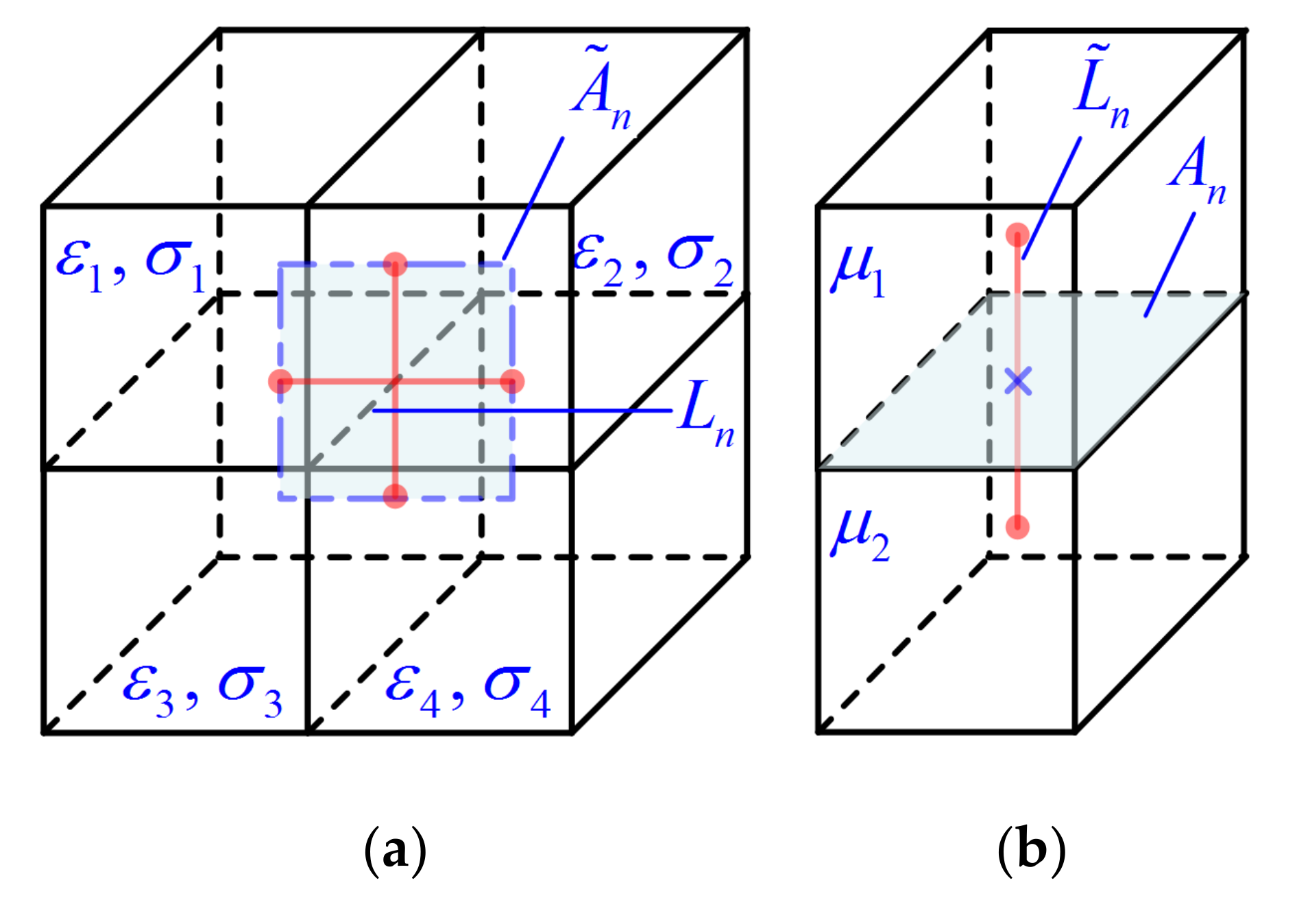
2.3. Discrete Material Relationship

According to the constitutive relations of continuous fields, for non-dispersive and isotropic (or orthotropic) materials, material matrices in the Yee-cell are diagonal [32]:

$${\left(D_{\epsilon }\right)}_{n,n}=\frac{{\stackrel{⌢}{\stackrel{⌢}{d}}}_n}{{\stackrel{⌢}{e}}_n}=\frac{{\displaystyle {\int }_{{\tilde{A}}_n}\mathit{D}\cdot d\mathit{A}}}{{\displaystyle {\int }_{L_n}\mathit{E}\cdot d\mathit{s}}}\approx \overline{\epsilon }\frac{{\tilde{A}}_n}{L_n},$$

(12)

$${\left(D_{\sigma }\right)}_{n,n}=\frac{{\stackrel{⌢}{\stackrel{⌢}{i}}}_n}{{\stackrel{⌢}{e}}_n}=\frac{{\displaystyle {\int }_{{\tilde{A}}_n}\mathit{J}\cdot d\mathit{A}}}{{\displaystyle {\int }_{L_n}\mathit{E}\cdot d\mathit{s}}}\approx \overline{\sigma }\frac{{\tilde{A}}_n}{L_n},$$

(13)

$${\left(D_{\mu }\right)}_{n,n}=\frac{{\stackrel{⌢}{\stackrel{⌢}{b}}}_n}{{\stackrel{⌢}{h}}_n}=\frac{{\displaystyle {\int }_{A_n}\mathit{B}\cdot d\mathit{A}}}{{\displaystyle {\int }_{{\tilde{L}}_n}\mathit{H}\cdot d\mathit{s}}}\approx \overline{\mu }\frac{A_n}{{\tilde{L}}_n},$$

(14)

where $D_{\epsilon }$, $D_{\sigma }$, and $D_{\mu }$ denote diagonal matrices of permittivity, conductivity, and permeability, respectively. Normally, matrix operators $D_{\epsilon }$ and $D_{\mu }$ are positive semi-definite and $D_{\sigma }$ is singular. $A_n$ and ${\tilde{A}}_n$ denote areas of the n-th primal facet and dual facet, respectively; $L_n$ and ${\tilde{L}}_n$ denote lengths of the n-th primal edge and dual edge, respectively. $\overline{\epsilon }$, $\overline{\sigma }$, and $\overline{\mu }$ denote material coefficients after properly weighted average.

Figure 4 illustrates the sub-cell averaging scheme, where the averaged permittivity and conductivity parameters are defined by the dual grid facet ${\tilde{A}}_i$ contained in the four adjacent primary grids having a common edge $L_i$ and the averaged permeability parameter is defined by the dual edge ${\tilde{L}}_k$ penetrating two adjacent primary grids having a common facet $A_k$.

The weighted average material coefficients $\overline{\epsilon }$, $\overline{\sigma }$, and $\overline{\mu }$ can be obtained as:

$${\overline{\epsilon }}_n=\left(A_{u,n}{\epsilon }_{u,n}+A_{u,n-M_v}{\epsilon }_{u,n-M_v}+A_{u,n-M_w}{\epsilon }_{u,n-M_w}+A_{u,n-M_v-M_w}{\epsilon }_{u,n-M_v-M_w}\right)/\left(4{\tilde{A}}_{u,n}\right),$$

(15)

$${\overline{\sigma }}_n=\left(A_{u,n}{\sigma }_{u,n}+A_{u,n-M_v}{\sigma }_{u,n-M_v}+A_{u,n-M_w}{\sigma }_{u,n-M_w}+A_{u,n-M_v-M_w}{\sigma }_{u,n-M_v-M_w}\right)/\left(4{\tilde{A}}_{u,n}\right),$$

(16)

$${\overline{\mu }}_n={\tilde{L}}_n/\left(\frac{L_{n-M_u}}{2{\mu }_{u,n-M_u}}+\frac{L_n}{2{\mu }_{u,n}}\right),$$

(17)

where $u=x,y,z;v=y,z,x;w=z,x,y$.

Obviously, discrete material relations are the only places where approximations are required in the spatial discretization process of Maxwell’s equations [29].

2.4. Explicit Updating Equations of TD-FIT

The semi-discrete Maxwell grid equations (MGE) and constitutive equations are [30]:

$$C\stackrel{⌢}{e}=-\frac{d}{dt}\stackrel{⌢}{\stackrel{⌢}{b}},\tilde{C}\stackrel{⌢}{h}={\stackrel{⌢}{\stackrel{⌢}{i}}}_{\mathrm{C}}+{\stackrel{⌢}{\stackrel{⌢}{i}}}_{\mathrm{S}}+\frac{d}{dt}\stackrel{⌢}{\stackrel{⌢}{d}},S\stackrel{⌢}{\stackrel{⌢}{b}}=0,\tilde{S}\stackrel{⌢}{\stackrel{⌢}{d}}=\stackrel{⌢}{\stackrel{⌢}{q}},$$

(18)

$$\stackrel{⌢}{\stackrel{⌢}{d}}=D_{\epsilon }\stackrel{⌢}{e},\stackrel{⌢}{\stackrel{⌢}{b}}=D_{\mu }\stackrel{⌢}{h},{\stackrel{⌢}{\stackrel{⌢}{i}}}_{\mathrm{C}}=D_{\sigma }\stackrel{⌢}{e},$$

(19)

where $\stackrel{⌢}{\stackrel{⌢}{q}}$ is the electric charge quantity, ${\stackrel{⌢}{\stackrel{⌢}{i}}}_{\mathrm{C}}$ and ${\stackrel{⌢}{\stackrel{⌢}{i}}}_{\mathrm{S}}$ are the loss term and source term of electric current, respectively.

To achieve second order accuracy for the two curl equations in MGE, temporal discretization is carried out with central difference. Then, explicit time-marching is performed by the staggered leap-frog (SLF) algorithm:

$${\stackrel{⌢}{e}}^{n+1}=\underset{¯}{CAE}\cdot {\stackrel{⌢}{e}}^n+\underset{¯}{CAH}\cdot \left(\tilde{C}{\stackrel{⌢}{h}}^{n+1/2}-{\stackrel{⌢}{\stackrel{⌢}{i}}}_{\mathrm{S}}^{n+1/2}\right),$$

(20)

$${\stackrel{⌢}{h}}^{n+1/2}={\stackrel{⌢}{h}}^{n-1/2}-\Delta t{D}_{\nu }C{\stackrel{⌢}{e}}^n,$$

(21)

where $D_{\nu }$ denotes diagonal matrices of magnetic reluctivity and it is the inverse matrix of $D_{\mu }$, $\Delta t$ denotes the time step and it should meet the Courant-Friedrichs-Lewy (CFL) stability constraint for stable time integration. Coefficients CAE and CAH in Equation (20) are expressed as:

$$\underset{¯}{CAE}=\left(\frac{D_{\epsilon }}{\Delta t}-\frac{D_{\sigma }}{2}\right)/\left(\frac{D_{\epsilon }}{\Delta t}+\frac{D_{\sigma }}{2}\right),$$

(22)

$$\underset{¯}{CAH}=1/\left(\frac{D_{\epsilon }}{\Delta t}+\frac{D_{\sigma }}{2}\right).$$

(23)

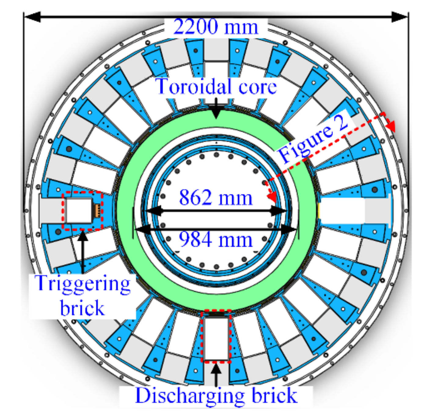
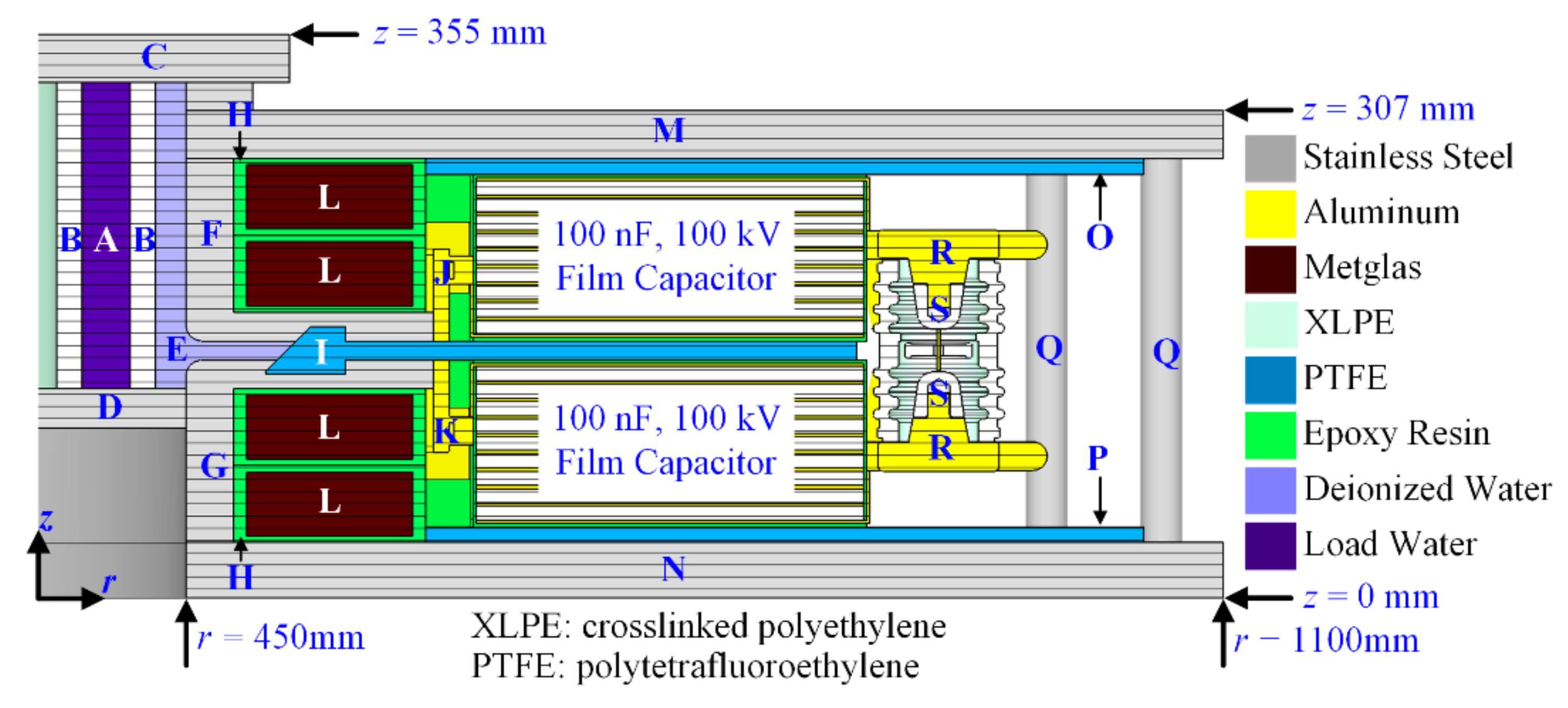
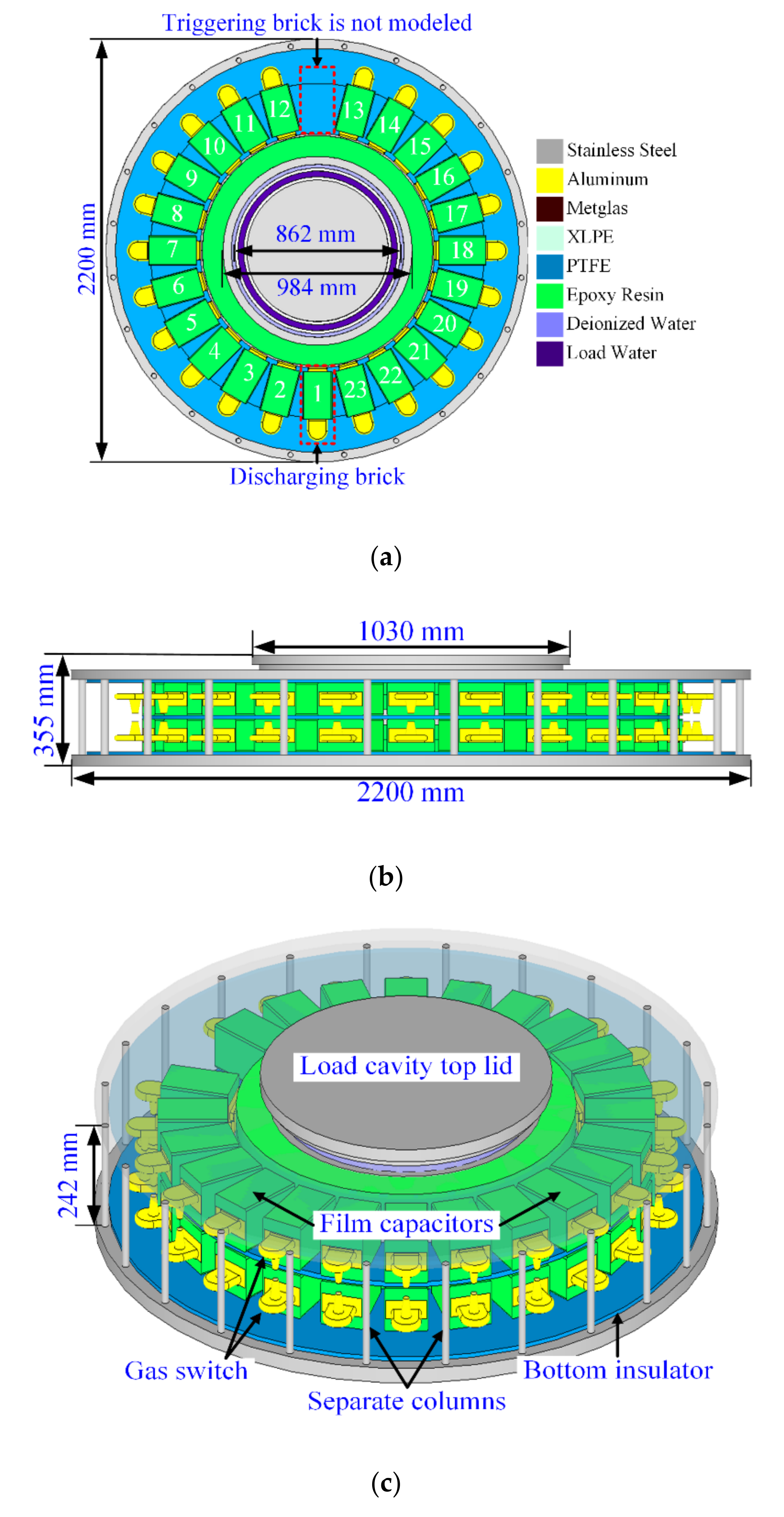
3. Numerical Model of the Single-Stage FLTD

Since FLTD with 24-separate columns is not rotationally symmetric, its three-dimensional model should be established for numerical calculation. As shown in Figure 5, the simulation model consists of 23 main discharging bricks (each brick includes two film capacitors and one gas switch), amorphous alloy magnetic core, epoxy resin casing for the core, PTFE and XLPE insulators, deionized water, stainless-steel induction cavity, 24 separate columns, and dummy load.

Table 1. Typical value of material characteristics in numerical calculations.

Components	Materials	Relative Permittivity	Relative Permeability	Electrical Conductivity (S/m)
FLTD cavity and separate columns	Stainless-steel	1.0	1.0	6.99 × 106
Capacitor/switch conductors	Aluminum	1.0	1.0	3.56 × 107
Magnetic core	Metglas	1.0	1000.0	8.13 × 10−5
Load cavity barrier	XLPE	2.3	1.0	0
Top/middle/bottom insulators	PTFE	2.1	1.0	0
Magnetic core outer casing	Epoxy resin	4.0	1.0	0
Deionized water filled cavity	Deionized water	80.0	1.0	5.55 × 10−6
0.1 Ω resistance dummy load	Water Solution	78.5	1.0	2.56 × 101
Background	Air	1.0	1.0	0

describes typical value of material characteristics in our numerical simulation.

Specifically, the amorphous alloy magnetic core used in this research is Metglas 2605TCA. Outer diameter and inner diameter of the toroidal core are 1184 mm and 976 mm, respectively. The magnetic core has four separate rings (item L in Figure 2), each ring being wound with 25-μm thick, 40-mm wide ribbon and silicon oxide (SiO2) insulating coating between each ribbon. The rings are annealed and then molded into epoxy resin casing (item H in Figure 2) to stabilize the turns and isolate the rings from each other.

Considering the complicated distribution of structures and materials and larger differences in spatial-scale of the FLTD cavity, some details in the engineering model that have little or no impact on field distribution should be ignored or simplified for successful computations [13,14,15,16]:

Small structures, for instance screws and holes that have negligible influence on the physical calculation results, are ignored.

Internal fine structures of the film capacitor are ignored, only equivalent capacitance, inductance, and resistance are considered and modeled.

The time-varying inductance/resistance of the conducting path of the triggered gas switch are simplified as a cylindrical conductor with constant inductance/resistance.

The toroidal core wound with amorphous alloy ribbons and SiO2 insulation coatings are simplified as homogeneous conductors with orthotropic conductivity and permeability. Moreover, the nonlinear hysteresis effect of magnetic core is ignored in simulations.

The triggering brick inside the induction cavity is not modeled. Assume that the trigger signal has been transmitted to the gas switches of discharging bricks in the same induction cavity.

The jitter and delay of the gas switch closure of discharging bricks are ignored. Suppose all the discharging bricks in the same cavity are turned on simultaneously.

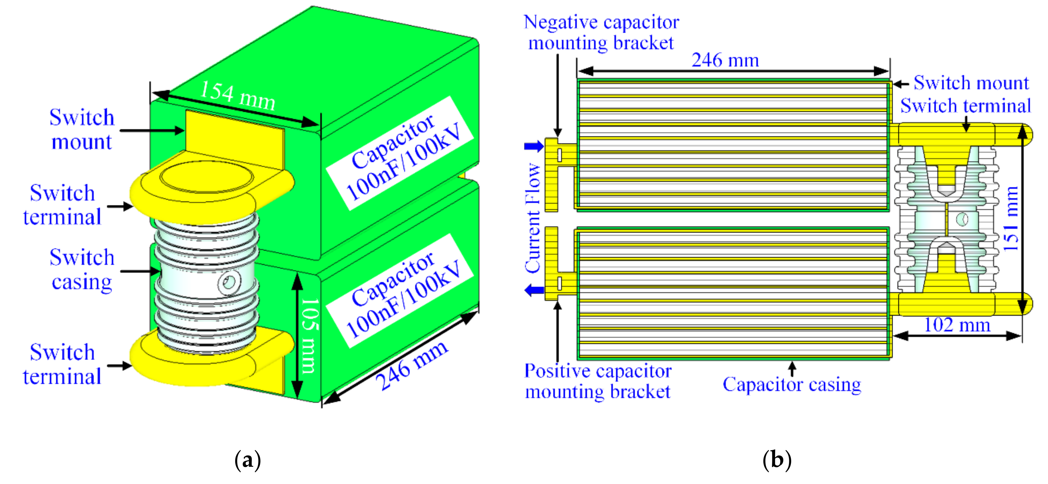
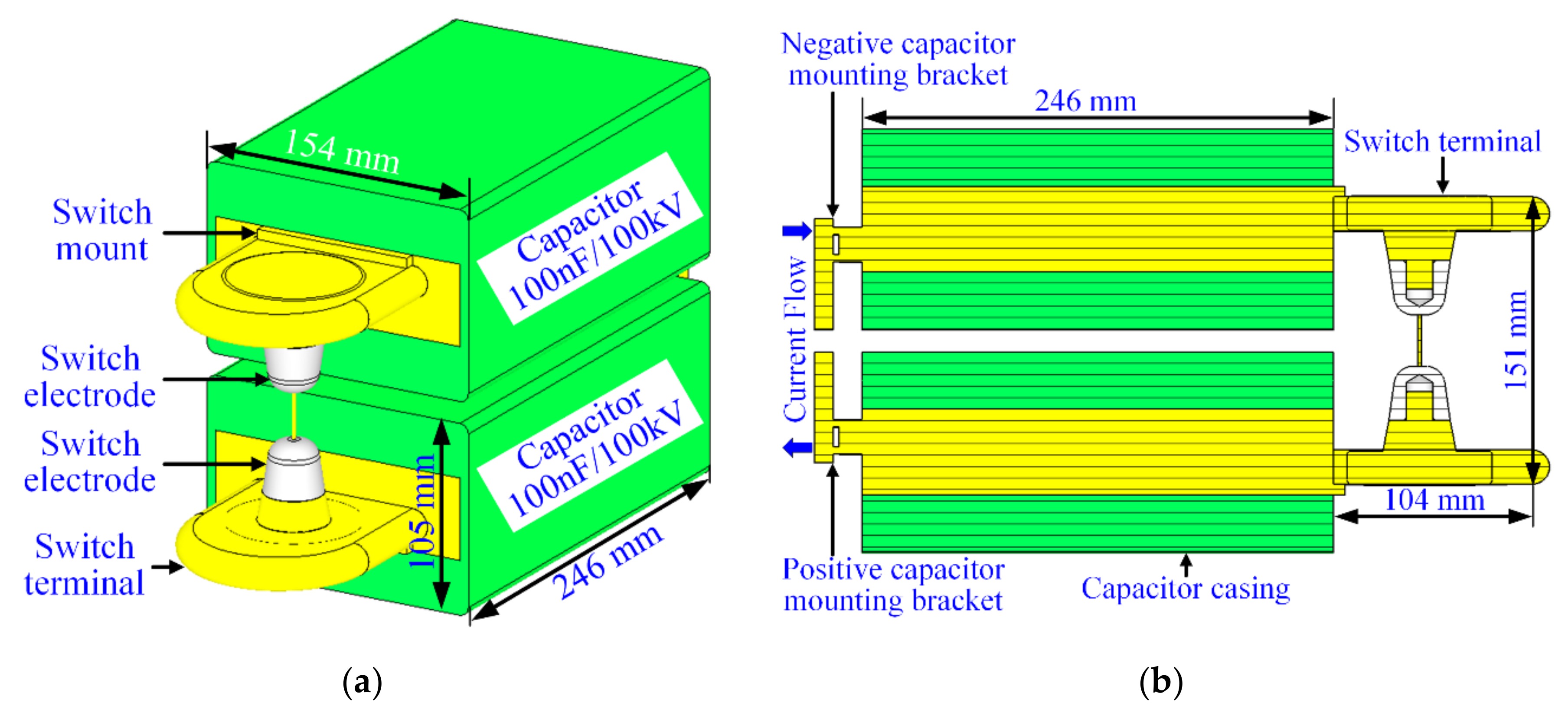
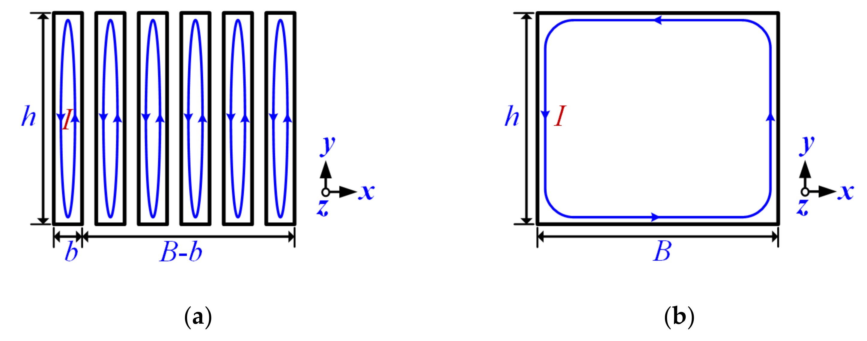
3.1. Simplified Model of Discharging Bricks

The simplification process of film capacitors and gas switch in a discharging brick is based on two principles [14]: the equivalent capacitance, inductance, and resistance should stay the same; the magnetic field distribution outside the brick model should remain unchanged.

Figure 6 shows the initial simplified model of discharging brick for finite element analysis, where a film capacitor is idealized as nine series-connected parallel-plate capacitors and the two electrodes of gas switch is connected by a thin cylindrical conductor. However, this model is still very complex in terms of number of DoFs and it needs further simplification for smooth transient EM field investigations on the FLTD cavity.

According to equivalent circuit model and measured results, capacitance, inductance, and resistance of a main discharging brick are 50 nF, 160 nH, and 0.3 Ω, respectively. We construct the 3-D model of a discharging brick to represent only its equivalent inductance and resistance, while its capacitance and initial voltage is represented by a lumped element in the circuit model. As shown in Figure 6, through finite element analysis, we can determine inductance and resistance of the brick model to be 160 nH and 0.3 Ω, respectively. The field model and circuit model are coupled through the conduction path of gas switch, as illustrated in Figure 7. The equivalent capacitance of the brick is modeled in circuit and it should be exactly 50 nF (two series-connected 100 nF capacitors).

To achieve the required electrical parameters and field distribution outside the brick, a genetic algorithm is used to optimize the shape and size of the internal equivalent conductor of the film capacitor. The final simplified model is shown in Figure 8. The main differences between the initial model and final model are the internal structure of film capacitor. However, they will exhibit the same brick discharge current due to the same electrical parameters. As can be observed from Figure 8, the current flow path and field distribution inside the capacitors will be different from those of the initial model. This is the tradeoff between accuracy and speed in our numerical calculation.

3.2. Equivalent Model of Toroidal Cores

This part will introduce a homogenization approach for wound magnetic cores with 25-μm thick ribbons and determination of electrical conductivity and permeability of the equivalent model.

Compared to the wound toroidal core, the simulation model with equivalent conductivity and permeability is determined based on the following two requirements [38]: the dissipated power must be equal; the magnetic field distribution outside the core must be the same.

Due to the skin effect [26], the eddy current flows only on the surface of the magnetic cores. Considering the aforementioned two requirements, resistance and current values between the original wound core model and equivalent solid conductor model should be equal, as shown in Figure 9.

The orthotropic conductivity and permeability of the homogeneous core are [38]:

$${\sigma }_x={\sigma }_{\mathrm{r}}{\left(b/h\right)}^2,{\sigma }_y={\sigma }_z={\sigma }_{\mathrm{r}},$$

(24)

$${\mu }_x=1/\left[F/{\mu }_0{\mu }_{\mathrm{r}}+\left(1-F\right)/{\mu }_0\right],{\mu }_y={\mu }_z=F{\mu }_0{\mu }_{\mathrm{r}},$$

(25)

where ${\sigma }_x$, ${\sigma }_y$, and ${\sigma }_z$ denote orthotropic conductivity of the solid conductor; ${\mu }_x$, ${\mu }_y$, and ${\mu }_z$ denote orthotropic permeability of the solid conductor; ${\sigma }_{\mathrm{r}}$ is isotropic conductivity of the magnetic core; $F$ is lamination filling factor; ${\mu }_0$ is permeability of free space; ${\mu }_{\mathrm{r}}$ is relative permeability of the core and it is chosen to be 1000 [6,37] in simulation.

The explicit modeling and full discretization of the magnetic core with a large number of ribbons is impractical, as this would result in a large number of grid elements (e.g., ~10 million) and a very small time step size. However, the equivalent model can significantly reduce computational cost and make reasonable approximations. Furthermore, the losses in the toroidal magnetic cores are modeled by a time-dependent resistor [37]:

$$R_{\mathrm{core}}(t)=\left(2S_0\sqrt{{\mu }_0{\mu }_{\mathrm{r}}{\rho }_{\mathrm{core}}}\right)/\left({\mathsf{\pi }}^{1.5}{r}_{\mathrm{core}}\delta \sqrt{t}\right),$$

(26)

where S₀ is the effective cross-sectional area of the magnetic core; ρ_core is the electrical resistivity of magnetic core; r_core is the average radius of the toroidal cores; δ is the thickness of the ribbon used to fabricate the cores; and t is the time instant.

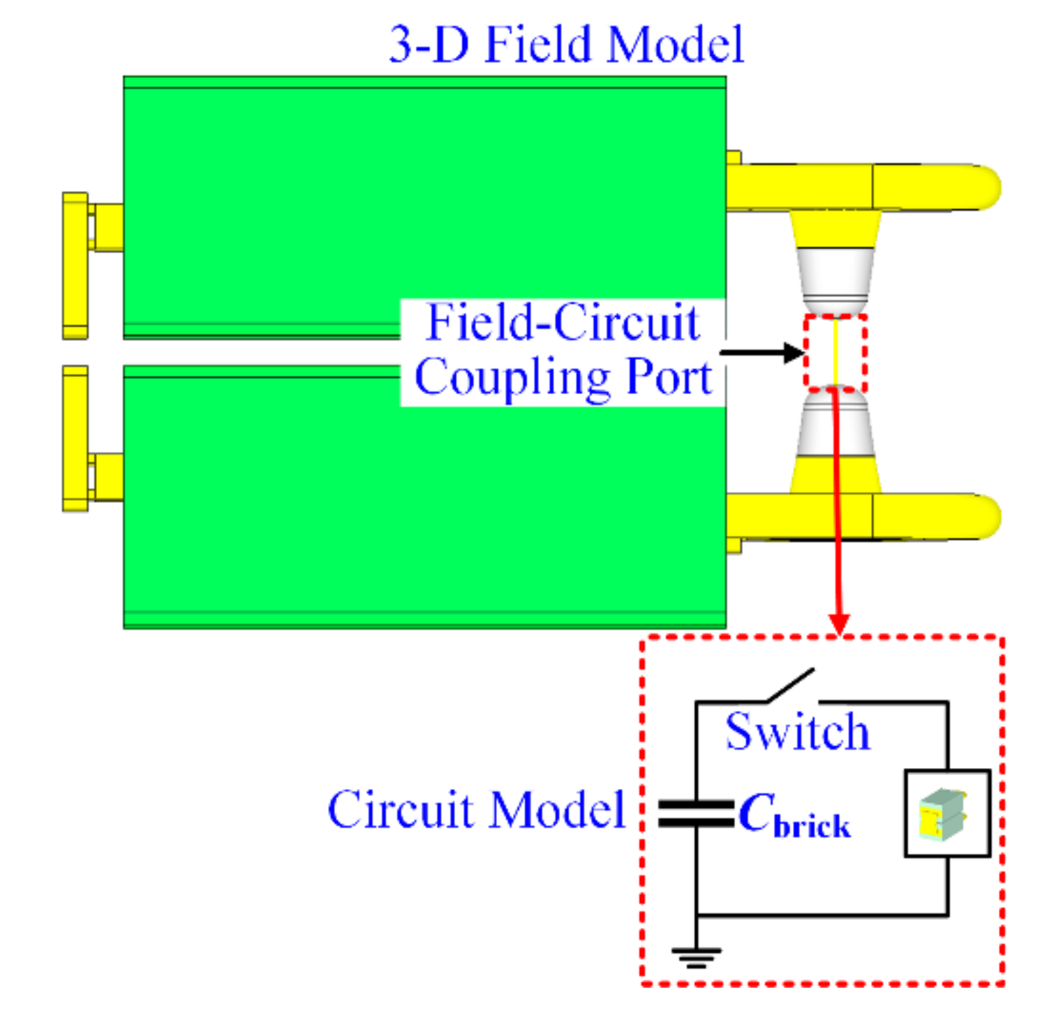
3.3. Field-Circuit Coupled TD-FIT

Because equivalent capacitance of the discharging brick is represented by a lumped element in the circuit model, the initial charging voltage of the lumped capacitor can be set according to requirement. As shown in Figure 7, when the switch in circuit model is turned on, pulsed discharge current generated by the lumped capacitor is coupled to the 3-D field model as excitations. The field-circuit coupling is achieved by adding a lumped element current term ${\stackrel{⌢}{\stackrel{⌢}{i}}}_{\mathrm{L}}$ to the right-hand side of the Ampère’s law [33]:

$$\tilde{C}\stackrel{⌢}{h}={\stackrel{⌢}{\stackrel{⌢}{i}}}_{\mathrm{C}}+{\stackrel{⌢}{\stackrel{⌢}{i}}}_{\mathrm{S}}+{\stackrel{⌢}{\stackrel{⌢}{i}}}_{\mathrm{L}}+\frac{d}{dt}\stackrel{⌢}{\stackrel{⌢}{d}}.$$

(27)

Suppose the lumped element with capacitance C are placed along the y-axis and between node (x_i, y_j+1, z_k) and node (x_i, y_j, z_k) of the primal grid, Equation (27) becomes:

$$\tilde{C}{\stackrel{⌢}{h}}^{n+1/2}=D_{\sigma }\frac{({\stackrel{⌢}{e}}^{n+1}+{\stackrel{⌢}{e}}^n)}{2}+{\stackrel{⌢}{\stackrel{⌢}{i}}}_{\mathrm{S}}^{n+1/2}+{\stackrel{⌢}{\stackrel{⌢}{i}}}_{\mathrm{L}}^{n+1/2}+D_{\epsilon }\frac{({\stackrel{⌢}{e}}^{n+1}-{\stackrel{⌢}{e}}^n)}{\Delta t},$$

(28)

$${\stackrel{⌢}{\stackrel{⌢}{i}}}_{\mathrm{L}}^{n+1/2}=\frac{C}{\Delta t}\left({\stackrel{⌢}{e}}_y^{n+1}(x_i,y_j,z_k)-{\stackrel{⌢}{e}}_y^n(x_i,y_j,z_k)\right).$$

(29)

Therefore, the lumped capacitor C only changes updating coefficients of the electric voltage (x_i, y_j, z_k) where the circuit model and 3-D field model are coupled. The SLF time-marching of the field-circuit coupled TD-FIT needs no other change.

3.4. Nonuniform Grid

For complex models, to ensure the computation precision, a finer mesh is required for accurate simulation of the small geometrical details. However, this results in an increase in the total number of DoFs and a decrease in the time step of the explicit updating of TD-FIT. Thus, the required computer resources and computation time will increase dramatically.

The nonuniform-grid or sub-grid technique can be employed as a solution, i.e., fine mesh is introduced only in regions where the EM field changes drastically while coarse mesh is used in the rest of the computational domain, accomplishing a good computational balance between accuracy and efficiency [39]. In the nonuniform grid, to minimize EM reflections and numerical dispersion, a transition sub-region with gradually changed mesh size should be set between the fine- and coarse-uniform sub-regions. In general, magnetic field components are still located at the midpoints of primal cell facets, whereas electric field components are off-centered between the two adjacent magnetic field components. Application of uniform grid only changes the facet’s area and edge’s length in Equations (15)–(17) and time step $\Delta t$.

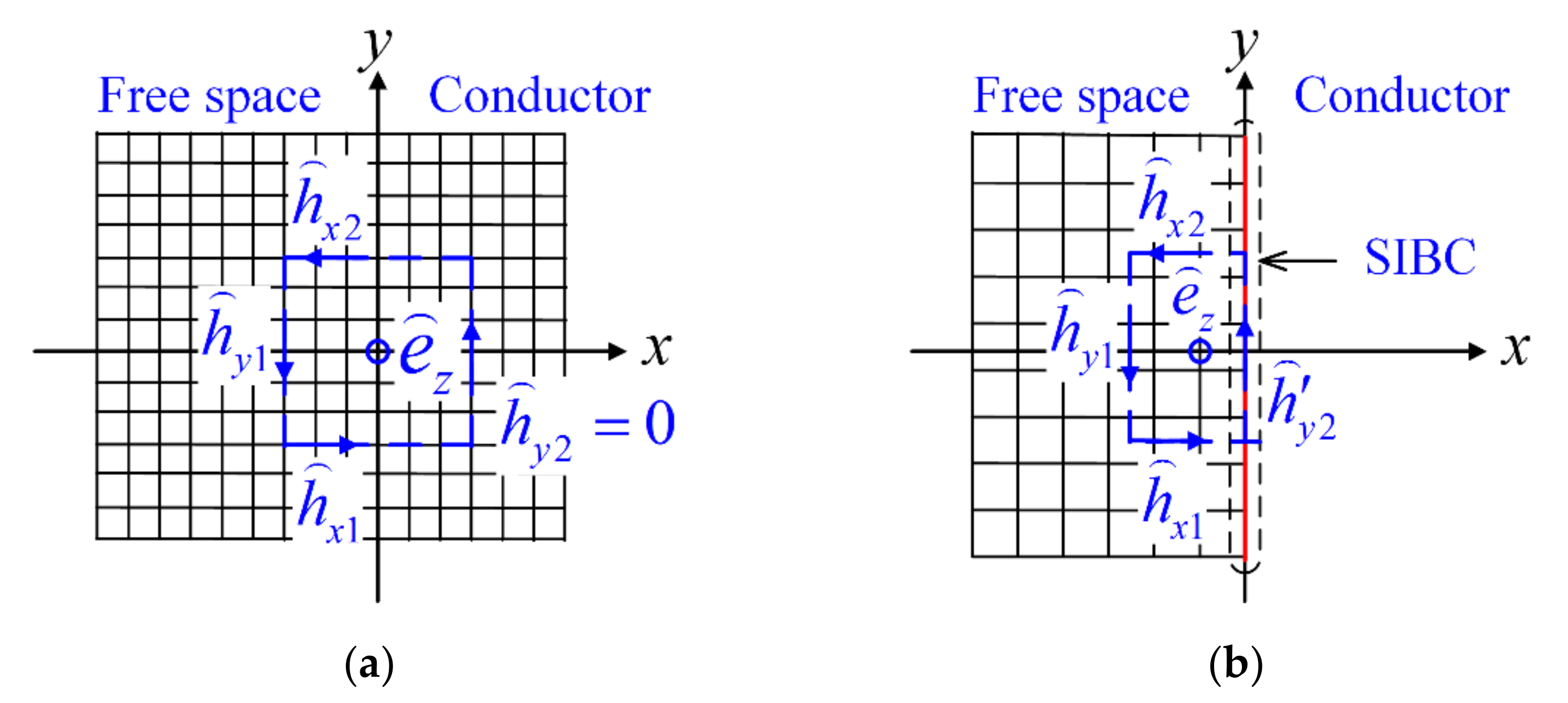
3.5. Surface Impedance Boundary Condition

Under the influence of a pulsed current with rise-time less than 100 ns, the skin depth of good conductors in the FLTD cavity is very small, leading to a rather short length of spatial step to accommodate the fast-changing field. As depicted in Figure 10, by using the SIBC, EM field distribution on the surface of conductors can be obtained without calculating the internal field distribution of the medium [40]. Therefore, introduction of the first-order SIBC in TD-FIT can effectively reduce the number of DoFs.

Since the SIBC is defined in the frequency domain, vector fitting techniques and first order rational functions are used for approximation of the convolution operation. Similar to the lumped element, surface equivalent current ${\stackrel{⌢}{\stackrel{⌢}{i}}}_{\mathrm{SIBC}}$ generated by the first-order SIBC is added to the right-hand side of Ampère’s law:

$$\tilde{C}{\stackrel{⌢}{h}}^{n+1/2}=D_{\sigma }({\stackrel{⌢}{e}}^{n+1}+{\stackrel{⌢}{e}}^n)/2+{\stackrel{⌢}{\stackrel{⌢}{i}}}_{\mathrm{S}}^{n+1/2}+{\stackrel{⌢}{\stackrel{⌢}{i}}}_{\mathrm{L}}^{n+1/2}+({\stackrel{⌢}{\stackrel{⌢}{i}}}_{\mathrm{SIBC}}^{n+1}+{\stackrel{⌢}{\stackrel{⌢}{i}}}_{\mathrm{SIBC}}^n)/2+D_{\epsilon }({\stackrel{⌢}{e}}^{n+1}-{\stackrel{⌢}{e}}^n)/\Delta t,$$

(30)

$${\stackrel{⌢}{\stackrel{⌢}{i}}}_{\mathrm{SIBC}}^{n+1}=c_0{\stackrel{⌢}{e}}^{n+1}+{\displaystyle \sum _{p=1}^P{\chi }_p^{n+1}},$$

(31)

$${\chi }_p^{n+1}=e^{-{\alpha }_p\Delta t}{\chi }_p^n+\frac{c_p}{{\alpha }_p}\left(1+\frac{e^{-{\alpha }_p\Delta t}-1}{{\alpha }_p\Delta t}\right){\stackrel{⌢}{e}}^{n+1}+\frac{c_p}{{\alpha }_p}\left[\frac{1}{{\alpha }_p\Delta t}-e^{-{\alpha }_p\Delta t}\left(1+\frac{1}{{\alpha }_p\Delta t}\right)\right]{\stackrel{⌢}{e}}^n,$$

(32)

where $P$ is the number of rational functions, $c_0$, $c_p$, and ${\alpha }_p$ denote coefficients and poles of the rational function approximation, respectively [40].

Obviously, Equation (30) is still an explicit update for the electric field and there is no need for reduction in the time step from the CFL stability limit.

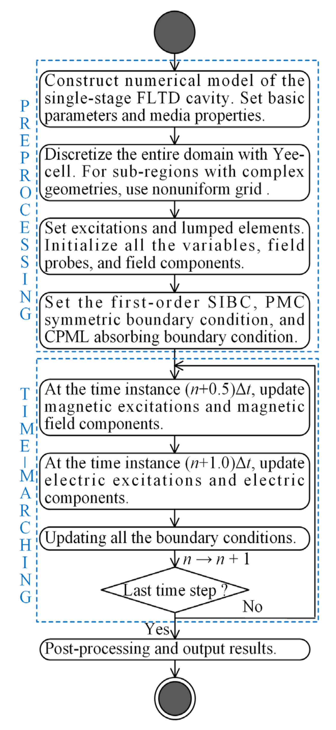
4. Results and Discussion

During the simulation, equivalent capacitance value of a single discharging brick is 50 nF and the initial charging voltage is 200 kV (±100 kV for each capacitor). The load resistance is set to 0.1 Ω. In FLTD cavity region, the maximum grid length is set to 1/30 of wavelength, while in the background region, the maximum grid length is set to 1/10 of wavelength. The obtained number of hexahedral primal grid of the single-stage FLTD with 24-separate columns is 5,116,608. The perfect magnetic conductor (PMC) boundary condition is implemented along the cut-plane because the FLTD cavity is symmetric along this direction. Outer boundary of the computational domain is the convolution perfectly matched layer (CPML) absorbing boundary condition and in every axis direction there are four cells. The flow chart including all the steps in the field-circuit coupled simulation is illustrated in Figure 11. All the simulations are accomplished by MATLAB and CST Studio Suite.

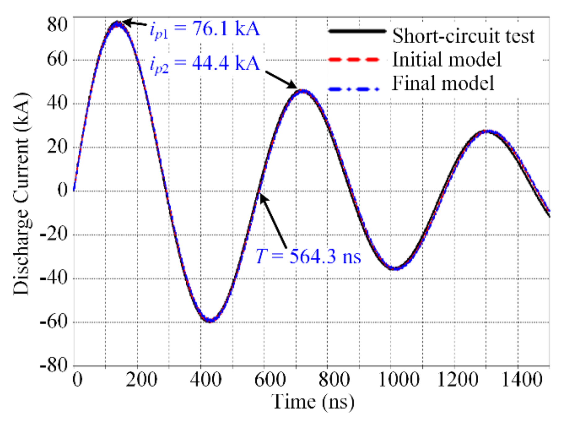
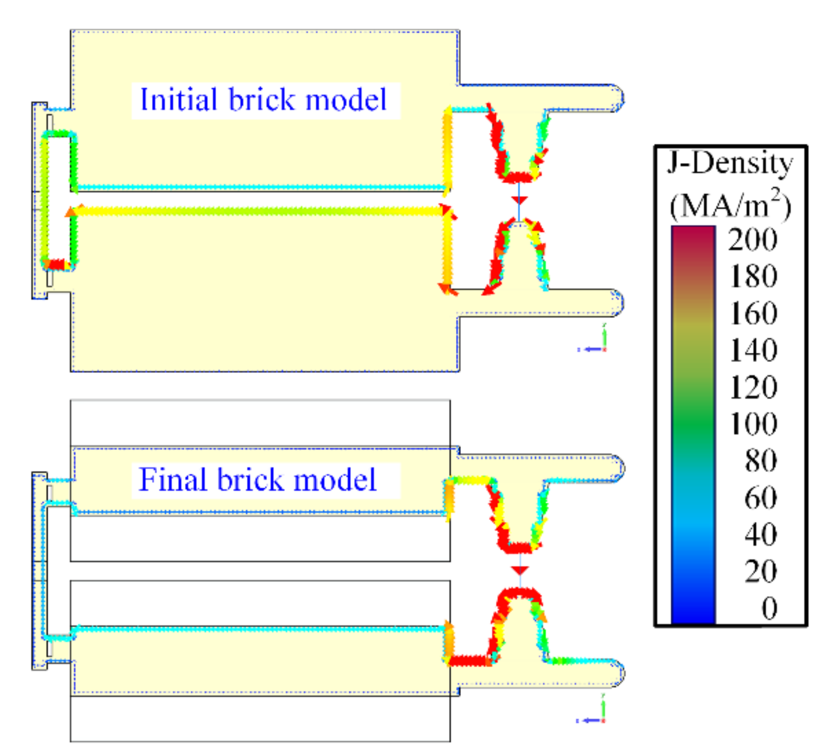
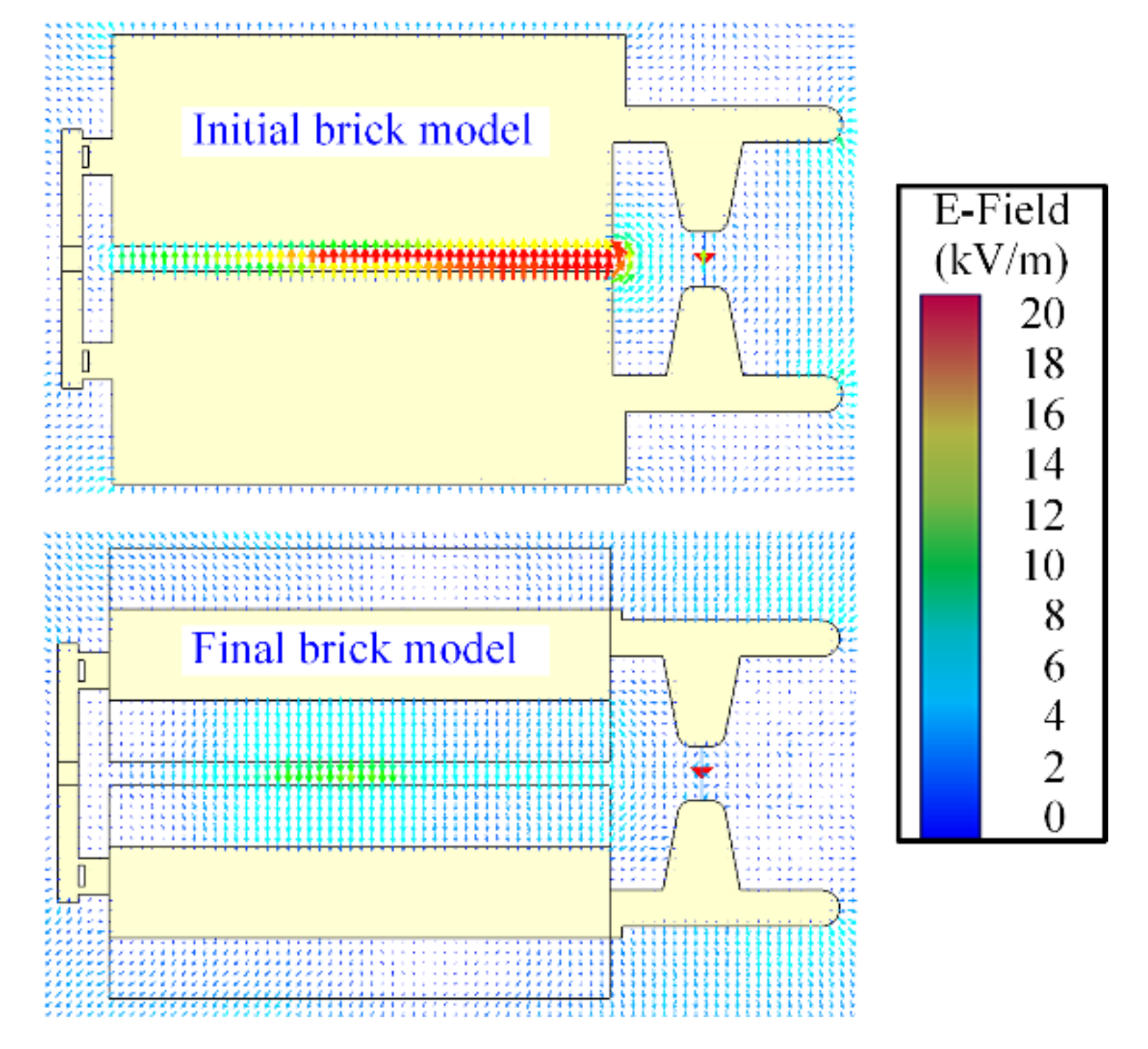
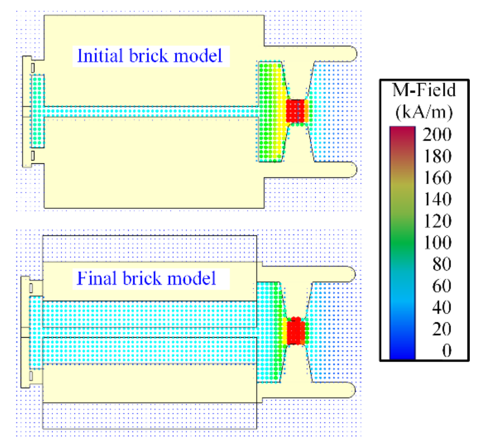
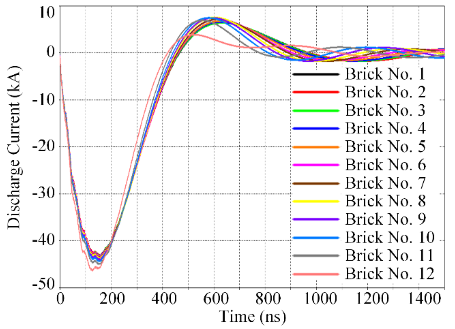
4.1. Performance of a Single Discharging Brick

Electric field intensity distribution when the two capacitors in a brick are initially charged to ±100 kV and the switch has not been triggered is shown in Figure 12. The electric field between the plus electrode and minus electrode is uniformly distributed and field intensity around edge of the electrode is lower than that of the middle part. Because the construction details of capacitors are not included in the field model, the fringe electric field intensity around the capacitors is obviously not a precise representation of the actual electric field around the physical capacitors.

The most important performance parameters of a discharging brick are amplitude and rise time of discharging current. In addition, the equivalent electrical parameters, peak current, and physical size of a brick determines the overall electrical performance of FLTD. The current of the single discharging brick is measured and simulated via the short-circuit discharge method. Equivalent inductance and resistance are obtained from the current waveform:

$$L=T^2/C\left[4{\mathsf{\pi }}^2+{\left(\ln \frac{i_{p1}}{i_{p2}}\right)}^2\right],$$

(33)

$$R=\frac{2L}{T}\ln \frac{i_{p1}}{i_{p2}},$$

(34)

where $T$ is the period of under-damped oscillation waveform of the current, $C$ is the capacitance (50 nF), $i_{p1}$ is the value of the first peak current and $i_{p2}$ is the value of the second peak current.

Figure 13 shows the short-circuit current waveform of a single discharging brick under experiment and simulation, which demonstrates good agreement with each other. The equivalent inductance and resistance can be calculated to be 160.1 nH and 0.3 Ω. Figure 14, Figure 15 and Figure 16 show the current path (current density vector), electric field intensity vector, and magnetic field intensity vector at the instant of maximum short-circuit discharging current of the two brick models. The current path of the two brick models is clearly very different because of the conductor shape in film capacitors. Most of the electric field distributes along the axial direction in the two brick models. However, the distributions in the regions of switch terminals and middle insulator demonstrate some differences, as shown in Figure 15. The magnetic field entirely along the azimuthal direction and the distribution pattern between the two brick models is very close. Although the two models have different current path, their short-circuit discharging current waveforms are in good agreement as depicted in Figure 13, because of the same equivalent electrical parameters in the field-circuit coupling models.

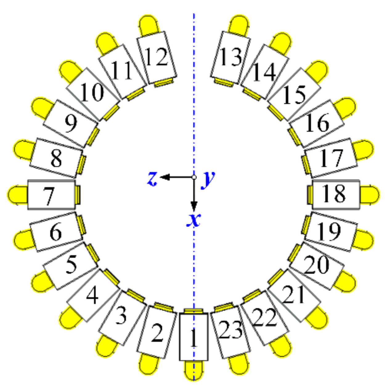
4.2. Equivalent Inductance of the 23 Discharging Bricks

When all the 23 discharging bricks in the same FLTD cavity begin to release the stored energy in the capacitors, due to the discharge current flow direction, all the mutual flux-linkages among different discharging bricks have the azimuthal direction, resulting in the increased total equivalent inductance of the discharging bricks. As depicted in Figure 17, the bricks No. 2 to 12 are symmetric to the bricks No. 23 to 13. Thus, only inductances of No. 1 to 12 bricks are calculated in simulation and the results are tabulated in

Table 2. Equivalent inductances of different discharging bricks when simultaneous discharged.

Brick No.	Total Inductance (nH)	Self-Inductance (nH)	Mutual-Inductance (nH)
1	195.8	160.1	35.7
2	194.3	160.1	34.2
3	194.2	160.1	34.1
4	194.2	160.1	34.1
5	194.1	160.1	34.0
6	194.2	160.1	34.1
7	195.6	160.1	35.5
8	194.3	160.1	34.2
9	195.1	160.1	35.0
10	193.7	160.1	33.6
11	193.2	160.1	33.1
12	182.6	160.1	22.5

.

It can be observed from Table 2 that brick No. 1 has the largest total inductance while brick No. 12 has the smallest total inductance. Obviously, brick No. 1 has the largest mutual flux-linkage since it located in the middle of all the discharging bricks, bricks No. 12 and 13 have the smallest mutual flux-linkage because of the location of the triggering brick. Therefore, when the FLTD induction cavity is releasing the stored energy, the actual equivalent inductance of the discharging brick is ~195 nH rather than 160 nH. This will lead to a larger load current rise time. The influence of increased brick’s equivalent inductance should be considered in the design of FLTD cavity.

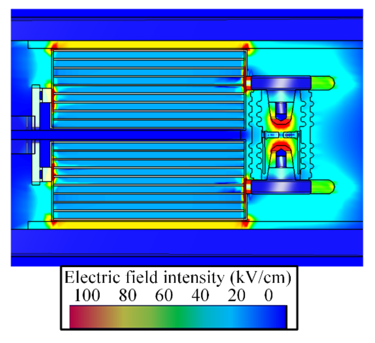
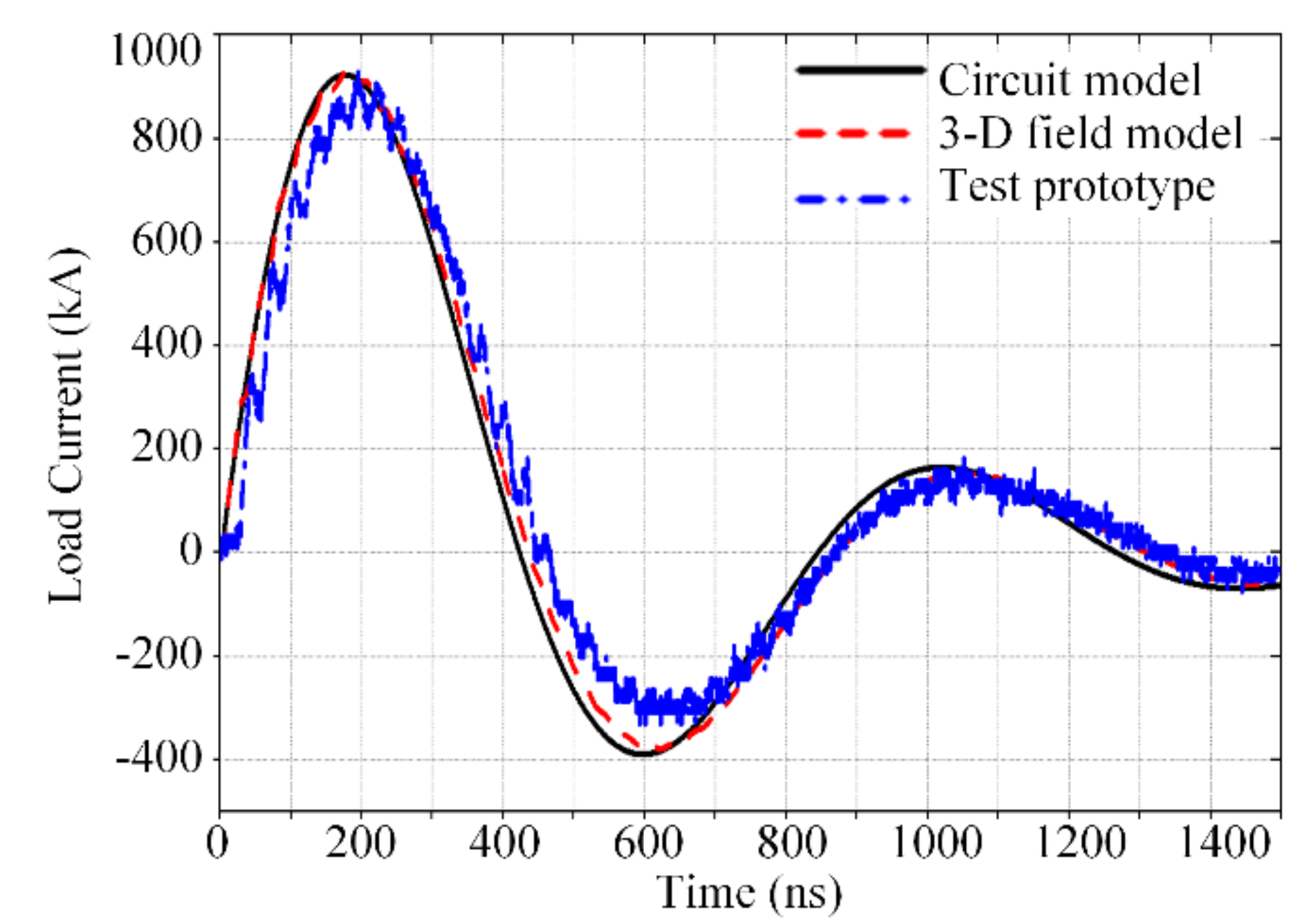
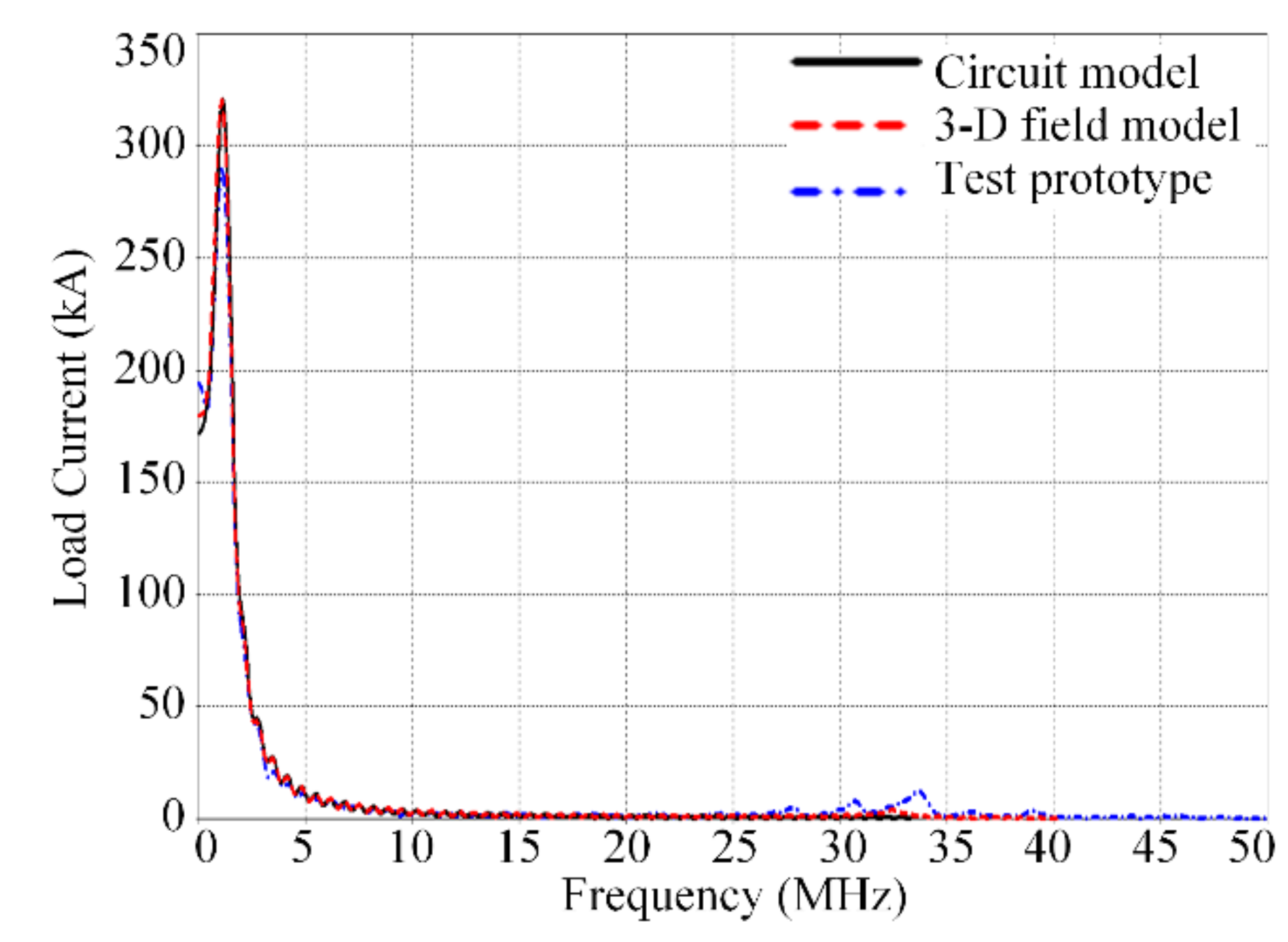
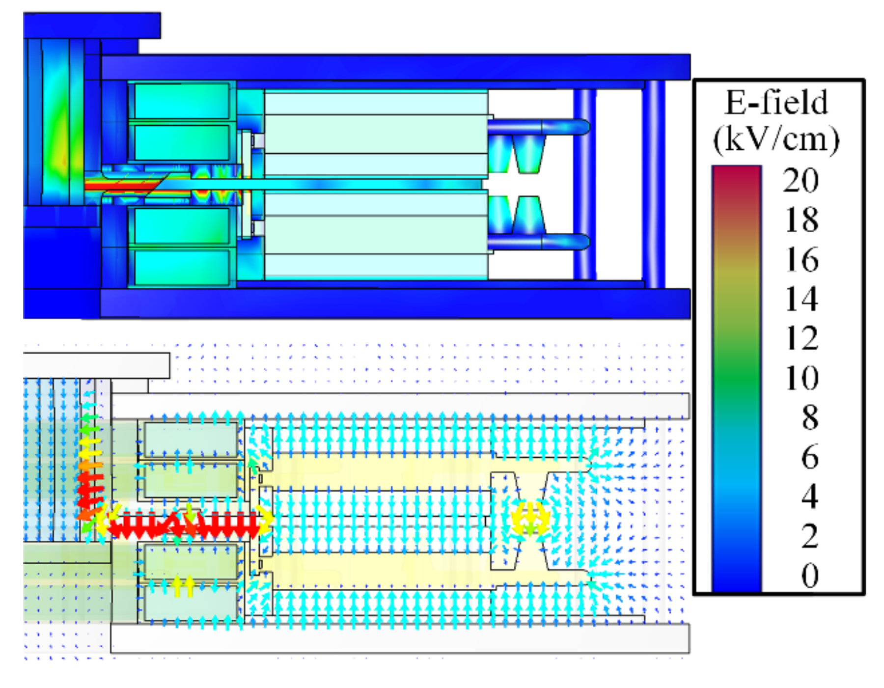
4.3. Performance of the Single-Stage FLTD Cavity

Figure 18 depicts load current generated by the experimental prototype, 3-D field model, and circuit model. In both simulations and experiments, the two capacitors in a discharging brick are charged to ±80 kV and the load resistance is set to 0.05 Ω. The rise time (10% to 90%) and amplitude of the load current is ~110 ns and ~950 kA, respectively. Thus, the MA-class single stage FLTD with 24-separate columns can generate required output current for the multi-stage series-connected FLTD module. By using the fast Fourier transform (FFT), the load current waveforms can be transformed from time domain to frequency domain, as illustrated in Figure 19. The simulated waveforms are in accordance with the experiment results except for low frequencies between 0–0.5 MHz and high frequencies between 26–35 MHz. Most of the spectral components of load current are in the range of 0 to 5 MHz. The discrepancies between simulations and measurements in the high frequency range are probably the effects of stray capacitances in the FLTD cavity. As shown in Figure 20, bricks’ discharge currents demonstrate that brick no. 12 has the smallest rise time and highest peak value, which conform to the smallest equivalent inductance of brick no. 12 in Table 2. Moreover, the circuit-field coupled TD-FIT only needs 3 h, 32 min calculation time and 3.7 GB memory consumption to complete the whole simulation. This is efficient to the 3-D time-domain simulation with over 10 million DoFs.

The cross-sectional view of electric- and magnetic-field intensity distributions at the time instant of maximum load voltage and load current are illustrated in Figure 21 and Figure 22, respectively. The electric field mainly distributes along the axial direction in the primary side and radial direction in the secondary side, whereas the magnetic field distributes along the azimuthal direction in both the primary and secondary sides. The EM wave propagates along the axial direction in the de-ionized water insulated transmission line of the secondary side of FLTD cavity, thus it operates in the transverse EM (TEM) wave mode. The highest magnitude of electric field intensity is now located near the narrow water-insulator interface region. The leakage magnetic flux is located in the middle insulator and the region of deionized water, which conforms to the theoretical analysis.

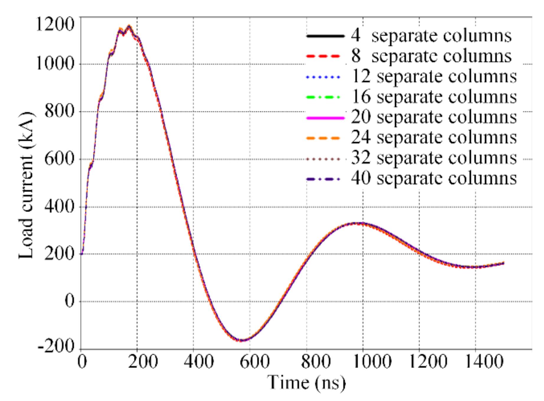
4.4. Influence of Separate Columns on the Output Performance

Currently, the number of uniformly arranged separate columns is set to 24. Here we change the number of separate columns to 4, 8, 12, 16, 20, 24, 32, and 40, and the resultant load current is shown in Figure 23. The inductance of a single separate column is ~126.7 nH. When multiple separate columns are used for the current return path and mechanical support, they are connected in parallel, and the equivalent inductance of these separate columns is further reduced. Compared to the magnetizing inductance of the FLTD cavity of ~10 μH, the structural inductance of the separate columns is very small. Therefore, the number of separate columns has negligible influence on the output performance of FLTD cavity, as can be indicated from Figure 23. Moreover, the diameter of the separate columns has been changed for parametric sweep simulations and it also has negligible influence on the load current of the FLTD cavity. Therefore, the 24-separate columns can replace the outer cylindrical wall without influencing the output electrical performances of FLTD.

5. Conclusions

In this contribution, the numerical model of the single-stage FLTD with 24-separate columns is established by using the field-circuit coupled time-domain finite integration theory. Combined with the nonuniform grid and first-order SIBC, the pulsed discharge process of the FLTD cavity is calculated with accuracy and efficiency. Applicability of the field-circuit coupled TD-FIT for performance analysis of FLTD is verified by experiments. For the first time, we have demonstrated that, due to the influence of mutual flux linkage among neighboring discharging bricks, equivalent inductance of the discharging brick will increase by ~35 nH when all of them are triggered synchronously. The 24 separate columns have negligible impact on the output performance of FLTD and can replace the traditional outer cylindrical wall. With the ±80 kV initial capacitor charge voltage and 0.05 Ω load resistance, the rise time and amplitude of load current are ~110 ns and ~0.95 MA, respectively. Electromagnetic characteristics of the discharging bricks and FLTD induction cavity have also been revealed. In the near future, we will focus on the accurate modeling of spatial multi-scale and nonlinear structures (such as magnetic cores ribbons, film capacitors) in the FLTD induction cavity and electromagnetic-thermal-mechanical coupled analysis during the discharging process.

References

1. Piovesan, P. RFX-mod: A multi-configuration fusion facility for three-dimensional physics studies. Phys. Plasmas 2013, 7220, 056112. [Google Scholar] [CrossRef]
2. Ryutov, D.D.; Derzon, M.S.; Matzen, M.K. The physics of fast Z pinches. Rev. Mod. Phys. 2000, 72, 167–223. [Google Scholar] [CrossRef] [Green Version]
3. Spielman, R.B.; Froula, D.; Brent, G.; Campbell, E.; Reisman, D.; Savage, M.; Shoup, I.M.; Stygar, W.; Wisher, M. Conceptual design of a 15-TW pulsed-power accelerator for high-energy-density–physics experiments. Matter Radiat. Extrem. 2017, 2, 204–223. [Google Scholar] [CrossRef] [Green Version]
4. Douglass, J.D.; Hutsel, B.T.; Leckbee, J.J.; Mulville, T.D.; Stoltzfus, B.S.; Wisher, M.L.; Savage, M.E.; Stygar, W.A.; Breden, E.W.; Calhoun, J.D.; et al. 100 GW linear transformer driver cavity: Design, simulations, and performance. Phys. Rev. Accel. Beams 2018, 21, 120401. [Google Scholar] [CrossRef] [Green Version]
5. Wang, Z.; Sun, F.; Qiu, A.; Hu, L.; Yin, J.; Cong, P.; Jiang, X.; Wei, H.; Jiang, H. A 80 kV gas switch triggered by a 17 μJ fiber-optic laser. Rev. Sci. Instrum. 2020, 91, 056104. [Google Scholar] [CrossRef] [PubMed]
6. Sun, F.; Zeng, J.; Liang, T.; Wei, H.; Jiang, X.; Wang, Z.; Yin, J.; Qiu, A. A novel triggering technique based on an internal brick and azimuthal line in cavities for linear transformer drivers. Mod. Appl. Phys. 2016, 7, 010401. (In Chinese) [Google Scholar]
7. Sun, F.; Jiang, X.; Wang, Z.; Wei, H.; Qiu, A. Design and simulation of fast linear transformer driver with four stages in series sharing common cavity shell and mega-ampere current. High Power Laser Part. Beams 2018, 30, 035001. (In Chinese) [Google Scholar]
8. Koval’chuk, B.M.; Vizir’, V.A.; Kim, A.A.; Kumpyak, E.V.; Loginov, S.V.; Bastrikov, A.N.; Chervyakov, V.V.; Tsoi, N.V.; Monjaux, P.; Kh’Yui, D. Fast primary storage device utilizing a linear pulse transformer. Russ. Phys. J. 1997, 40, 1142–1153. [Google Scholar] [CrossRef]
9. Guo, F.; Zou, W.; Gong, B.; Jiang, J.; Chen, L.; Wang, M.; Xie, W. Modeling power flow in the induction cavity with a two dimensional circuit simulation. Phys. Rev. Accel. Beams 2017, 20, 020401. [Google Scholar] [CrossRef]
10. Liu, P.; Sun, F.; Wei, H.; Wang, Z.; Yin, J.; Qiu, A. Influences of switching jitter on the operational performances of linear transformer drivers-based drivers. Plasma Sci. Technol. 2012, 14, 347–352. [Google Scholar] [CrossRef] [Green Version]
11. Zhang, L.; Meng, W.; Zhou, L.; Tian, Q.; Guo, F.; Wang, L.; Qing, Y.; Zhao, Y.; Dai, Y.; Han, W.; et al. Development of a hybrid mode linear transformer driver stage. Phys. Rev. Accel. Beams 2018, 21, 020401. [Google Scholar] [CrossRef] [Green Version]
12. Zhou, Q.; Li, Y.; Wang, X.; Zou, X. Full circuit simulation and optimization design for Z-800. High Volt. Eng. 2020, 46, 2610–2615. (In Chinese) [Google Scholar]
13. Rose, D.V.; Miller, C.L.; Welch, D.R.; Clark, R.; Madrid, E.A.; Mostrom, C.B.; Stygar, W.A.; Lechien, K.R.; Mazarakis, M.A.; Langston, W.L.; et al. Circuit models and three-dimensional electromagnetic simulations of a 1-MA linear transformer driver stage. Phys. Rev. ST Accel. Beams 2010, 13, 090401. [Google Scholar] [CrossRef] [Green Version]
14. Wei, H.; Sun, F.; Qiu, A.; Yin, J.; Zeng, J.; Hu, Y.; Liang, T. Simulation analysis of transformer oil and glycerin as dielectric medium in inductive voltage adders. IEEE Trans. Dielectr. Electr. Insul. 2014, 21, 1778–1783. [Google Scholar] [CrossRef]
15. Wei, H.; Sun, F.; Yin, J.; Hu, Y.; Liang, T.; Cong, P.; Qiu, A. Numerical simulation of azimuthal uniformity of injection currents in single-point-feed induction voltage adders. Plasma Sci. Technol. 2015, 17, 235–240. [Google Scholar] [CrossRef]
16. Reisman, D.B.; Stoltzfus, B.S.; Stygar, W.A.; Austin, K.N.; Waisman, E.M.; Hickman, R.J.; Davis, J.-P.; Haill, T.A.; Knudson, M.D.; Seagle, C.T.; et al. Pulsed power accelerator for material physics experiments. Phys. Rev. ST Accel. Beams 2015, 18, 090401. [Google Scholar] [CrossRef] [Green Version]
17. Bettini, P.; Specogna, R. Computation of stationary 3D halo currents in fusion devices with accuracy control. J. Comput. Phys. 2014, 273, 100–117. [Google Scholar] [CrossRef]
18. Yanovskiy, V.V.; Isernia, N.; Pustovitov, V.D.; Villone, F.; Abate, D.; Bettini, P.; Chen, S.L.; Havlicek, J.; Herrmann, A.; Hromadka, J.; et al. Comparison of approaches to the electromagnetic analysis of COMPASS-U vacuum vessel during fast transients. Fusion Eng. Des. 2019, 146, 2338–2342. [Google Scholar] [CrossRef]
19. Gourdain, P.A.; Adams, M.B.; Evans, M.; Hasson, H.R.; Shapovalov, R.V.; Spielman, R.B.; Young, J.R.; West-Abdallah, I. Current adding transmission lines for compact MA-class linear transformer drivers. Phys. Rev. Accel. Beams 2020, 23, 030401. [Google Scholar] [CrossRef] [Green Version]
20. Flisgen, T.; Gjonaj, E.; Glock, H.W.; Tsakanian, A. Generalization of coupled S-parameter calculation to compute beam impedances in particle accelerators. Phys. Rev. Accel. Beams 2020, 23, 034601. [Google Scholar] [CrossRef] [Green Version]
21. Yan, J.; Gou, Y.; Zhang, S.; Wang, G.; Chen, X.; Wang, Y.; Li, Z.; Shen, S.; Li, Q.; Ding, W. Output current optimization for multibrick parallel discharge drivers based on genetic algorithm. IEEE Trans. Plasma Sci. 2019, 47, 3015–3025. [Google Scholar] [CrossRef]
22. Voltolina, D.; Bettini, P.; Alotto, P.; Moro, F.; Torchio, R. High-performance PEEC analysis of electromagnetic scatters. IEEE Trans. Magn. 2019, 55, 7201204. [Google Scholar] [CrossRef]
23. Abate, D.; Bruno, C.; Chiariello Andrea, G.; Giuseppe, M.; Nicolò, M.; Stefano, M.; Guglielmo, R.; Salvatore, V.; Fabio, V. Fast and parallel computational techniques applied to numerical modeling of RFX-mod fusion device. ACES J. 2018, 33, 176–179. [Google Scholar]
24. Taflove, A.; Brodwin, M.E. Numerical solution of steady-state electromagnetic scattering problems using the time-dependent maxwell’s equations. IEEE Trans. Microw. Theory Tech. 1975, 23, 623–630. [Google Scholar] [CrossRef]
25. Biro, O.; Preis, K. On the use of the magnetic vector potential in the finite-element analysis of three-dimensional eddy currents. IEEE Trans. Magn. 1989, 25, 3145–3159. [Google Scholar] [CrossRef]
26. Yoshida, T.; Okuzono, T.; Sakagami, K. Time domain room acoustic solver with fourth-order explicit FEM using modified time integration. Appl. Sci. 2020, 10, 3750. [Google Scholar] [CrossRef]
27. Ruehli, A.E. Equivalent circuit models for three-dimensional multiconductor systems. IEEE Trans. Microw. Theory Tech. 1974, 22, 216–221. [Google Scholar] [CrossRef]
28. Le-Duc, T.; Meunier, G. 3-D integral formulation for thin electromagnetic shells coupled with an external circuit. Appl. Sci. 2020, 10, 4284. [Google Scholar] [CrossRef]
29. Weiland, T. On the numerical solution of Maxwell’s equations and applications in the field of accelerator physics. Part. Accel. 1984, 15, 245–292. [Google Scholar]
30. Lau, T.; Gjonaj, E.; Weiland, T. Time integration methods for particle beam simulations with the finite integration theory. Frequenz 2005, 59, 210–219. [Google Scholar] [CrossRef]
31. You, J.W.; Wang, H.G.; Zhang, J.F.; Cui, W.Z.; Cui, T.J. The conformal TDFIT-PIC method using a new extraction of conformal information (ECI) technique. IEEE Trans. Plasma Sci. 2013, 41, 3099–3108. [Google Scholar] [CrossRef]
32. Schnepp, S.M.; Gjonaj, E.; Weiland, T. Extension of the finite integration technique including dynamic mesh refinement and its application to self-consistent beam dynamics simulations. Phys. Rev. ST Accel. Beams 2012, 15, 014401. [Google Scholar] [CrossRef]
33. Schöps, S.; De Gersem, H.; Weiland, T. Winding functions in transient magneto-quasistatic field-circuit coupled simulations. COMPEL 2013, 32, 2063–2083. [Google Scholar] [CrossRef]
34. Udosen, N.I.; George, N.J. A finite integration forward solver and a domain search reconstruction solver for electrical resistivity tomography (ERT). Model. Earth Syst. Environ. 2018, 4, 1–12. [Google Scholar] [CrossRef]
35. Razi-Kazemi, A.A.; Hajian, M. Probabilistic assessment of ground potential rise using finite integration technique. IEEE Trans. Power Deliver. 2018, 33, 2452–2461. [Google Scholar] [CrossRef]
36. Mao, C.; Wang, X.; Zou, X.; Lehr, J. Investigation of monolithic radial transmission lines for Z-pinch. IEEE Trans. Plasma Sci. 2017, 45, 2639–2647. [Google Scholar] [CrossRef]
37. Qiu, H.; Wang, S.; Sun, F.; Wang, Z.; Zhang, N. Transient electromagnetic field analysis for the single-stage FLTD with two different configurations using the finite-element method and finite integration technique. IEEE Trans. Magn. 2020, 56, 7515805. [Google Scholar] [CrossRef]
38. Wang, J.; Lin, H.; Huang, Y.; Sun, X. A new formulation of anisotropic equivalent conductivity in laminations. IEEE Trans. Magn. 2011, 47, 1378–1381. [Google Scholar] [CrossRef]
39. Fazio, R.; Jannelli, A.; Agreste, S. A finite difference method on non-uniform meshes for time-fractional advection-diffusion equations with a source term. Appl. Sci. 2018, 8, 960. [Google Scholar] [CrossRef] [Green Version]
40. Makinen, R.M.; De Gersem, H.; Weiland, T. Frequency- and time-domain formulations of an impedance- boundary condition in the finite-integration technique. In Proceedings of the URSI/IEEE XXIX Convention on Radio Science (URSI 2004), Espoo, Finland, 1–2 November 2004. [Google Scholar]
Figure 1. Top-down illustration of the newly developed 1-mega-ampere (MA) single-stage fast linear transformer driver (FLTD) cavity with top lid and insulator removed.
Applsci 10 08301 g001
Figure 2. Cross-sectional view (r-z plane in cylindrical coordinate system) of the newly developed single-stage FLTD. A: load cavity filled with water solution, B: insulating barrier of the load, C: load cavity top lid, D: load cavity bottom lid, E: deionized water-filled cavity, F: negative output electrode, G: positive output electrode, H: epoxy resin casings for magnetic cores, I: middle insulator, J: negative capacitor mounting bracket, K: positive capacitor mounting bracket, L: four separate rings of the magnetic core, M: top lid of FLTD cavity, N: bottom lid of FLTD cavity, O: top insulator, P: bottom insulator, Q: separate columns (24 in total), R: switch terminals, S: switch electrodes.
Applsci 10 08301 g002
Figure 3. Allocation of electric and magnetic components in the dual grid cell-complex of finite integration theory (FIT).
Applsci 10 08301 g003
Figure 4. Construction of the material matrices. (a) The four cells involved in the average of permittivity and conductivity, (b) the two cells involved in the average of permeability.
Applsci 10 08301 g004
Figure 5. Numerical model of the single-stage FLTD with 24-separate columns. (a) Top view with cavity top lid and insulator removed, (b) side view, and (c) axonometric view with cavity top lid and insulator set to be transparent.
Applsci 10 08301 g005
Figure 6. Initial simplified model of the discharge brick. (a) Perspective view, (b) cut-away view.
Applsci 10 08301 g006
Figure 7. Schematic of the field-circuit coupling port for a single discharging brick.
Applsci 10 08301 g007
Figure 8. Finial simplified model of the discharge brick. (a) Perspective view, (b) cut-away view.
Applsci 10 08301 g008
Figure 9. Sectional view of current flow in the original model and equivalent model. (a) Ribbons with homogeneous conductivity, (b) Homogeneous core with orthotropic conductivity and permeability. ( h is width of the ribbon, b is thickness of a single ribbon, B is thickness of the solid conductor, and I is the magnitude of eddy current in magnetic core).
Applsci 10 08301 g009
Figure 10. Comparison of grids without and with the surface impedance boundary condition (SIBC). (a) Without SIBC, (b) with SIBC.
Applsci 10 08301 g010
Figure 11. Flow chart of numerical calculations based on the field-circuit coupled time-domain finite integration theory (TD-FIT).
Applsci 10 08301 g011
Figure 12. Cross-sectional view of magnitude of electric field intensity distribution of the discharging brick when initially charged.
Applsci 10 08301 g012
Figure 13. Simulated and measured short-circuit current waveform of a brick.
Applsci 10 08301 g013
Figure 14. Cross-sectional view of the current density vector at the instant of maximum brick current.
Applsci 10 08301 g014
Figure 15. Cross-sectional view of the electric field vector at the instant of maximum brick current.
Applsci 10 08301 g015
Figure 16. Cross-sectional view of the magnetic field vector at the instant of maximum brick current.
Applsci 10 08301 g016
Figure 17. Arrangement of the 23 discharging bricks and the corresponding brick number.
Applsci 10 08301 g017
Figure 18. Simulated and measured load current waveforms of the single-stage FLTD.
Applsci 10 08301 g018
Figure 19. Load current waveforms of the single-stage FLTD in the frequency domain.
Applsci 10 08301 g019
Figure 20. Simulated current waveforms of main discharging bricks of the single-stage FLTD.
Applsci 10 08301 g020
Figure 21. Cross-sectional view of the magnitude and vector diagram of electric field intensity at the instant of maximum load voltage.
Applsci 10 08301 g021
Figure 22. Cross-sectional view of the magnitude and vector diagram of magnetic field intensity at the instant of maximum load current.
Applsci 10 08301 g022
Figure 23. Simulated load current waveforms with the change of number of separate columns.
Applsci 10 08301 g023