Artificial Neural Network Modeling for Prediction of Dynamic Changes in Solution from Bioleaching by Indigenous Acidophilic Bacteria


Abstract
:1. Introduction
2. Materials and Methods
2.1. Information on Indigenous Acidophilic Bacteria Sampling and Cultivation of Reference Studies
2.2. Information on Bioleaching Experiments of Reference Studies
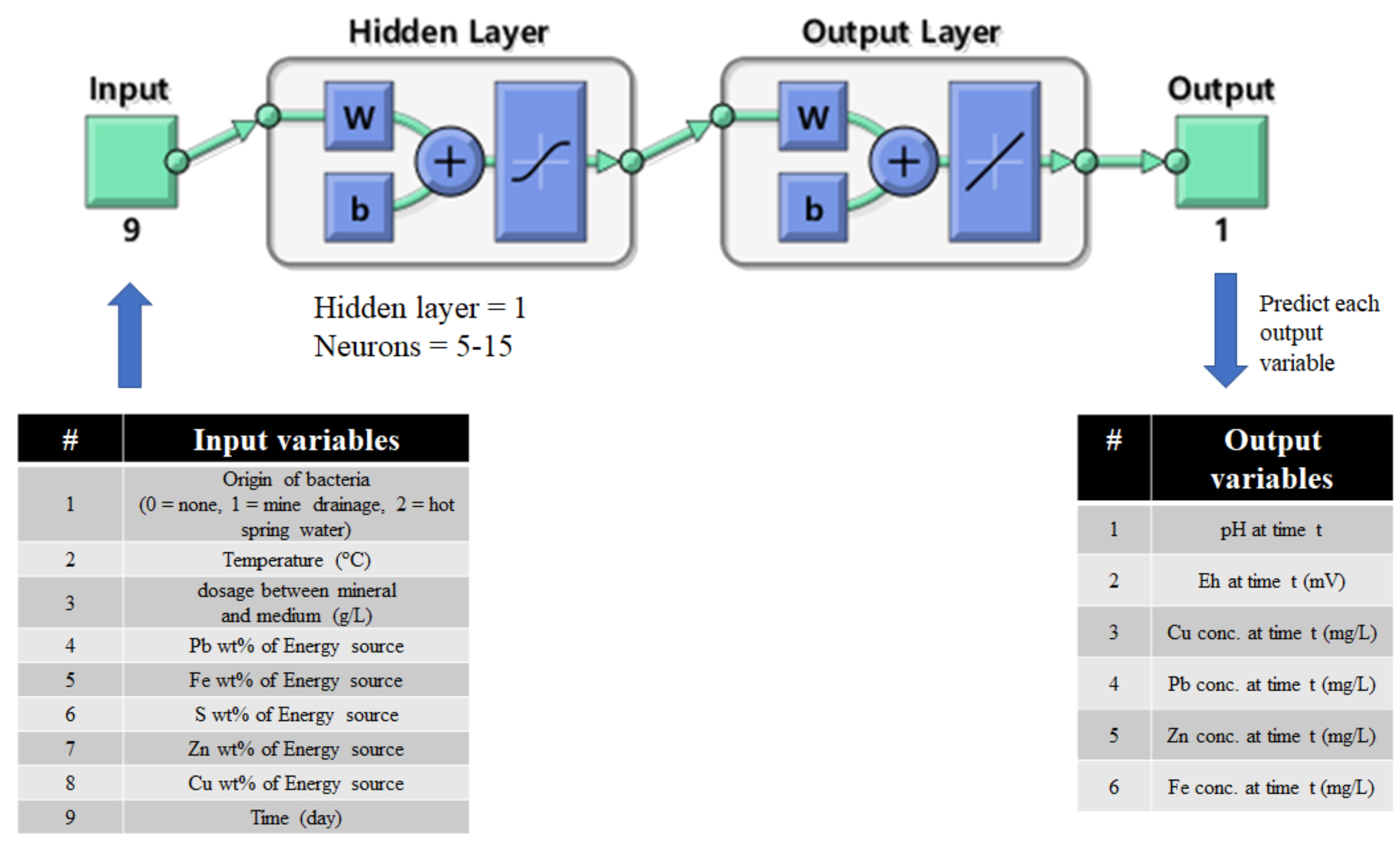
2.3. Artificial Neural Network Modeling
3. Results and Discussion
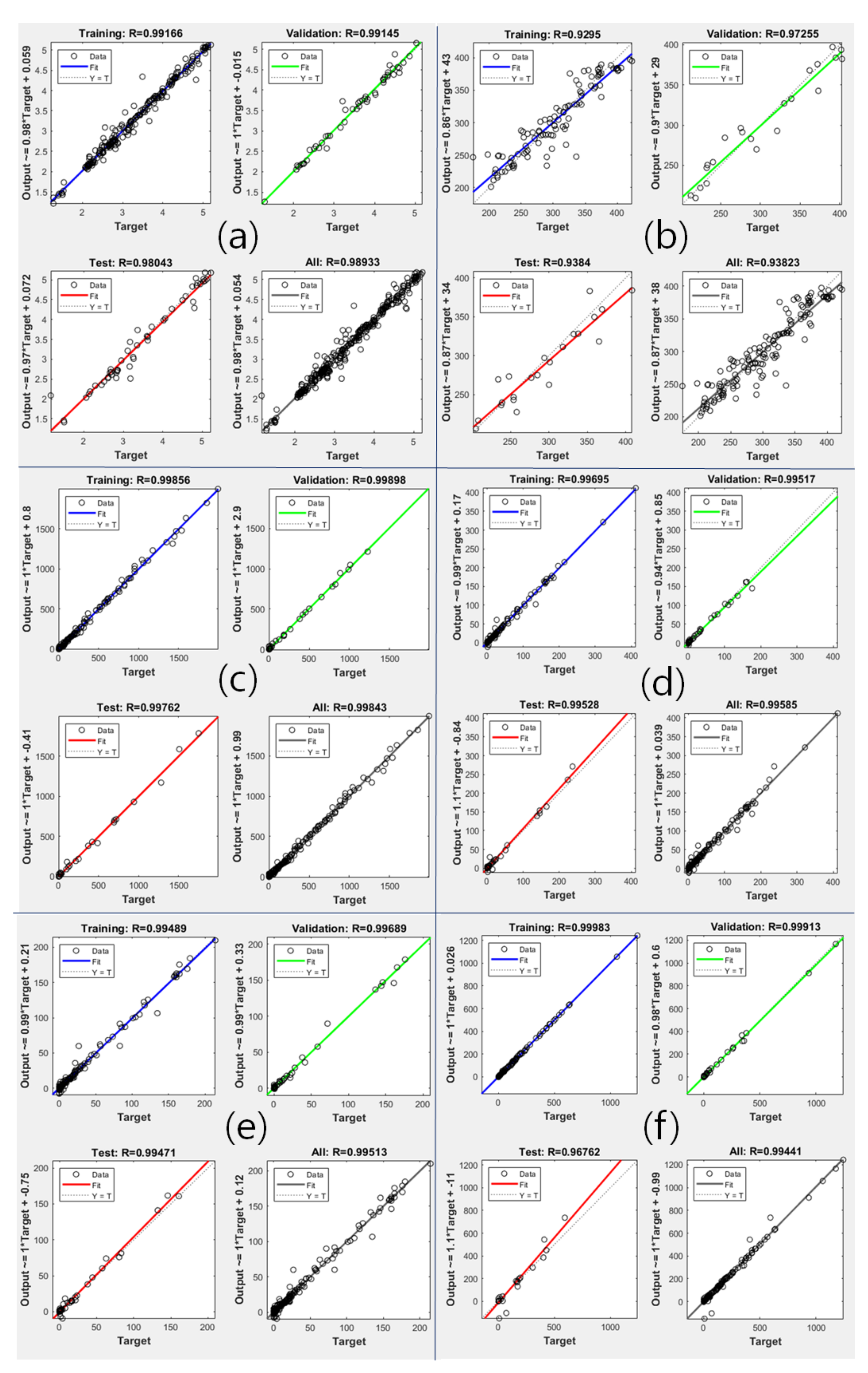
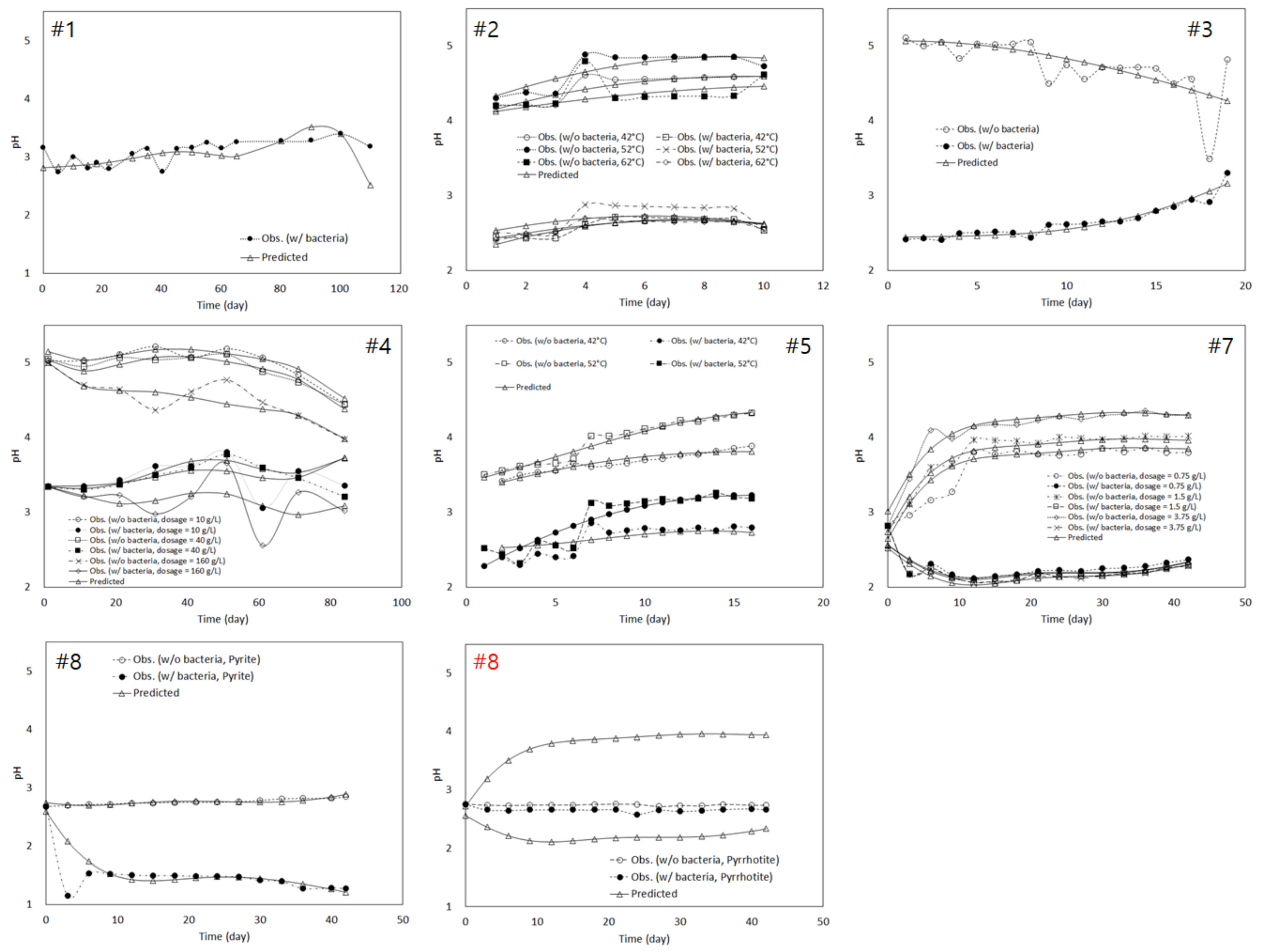
3.1. ANN Modeling for pH and Eh
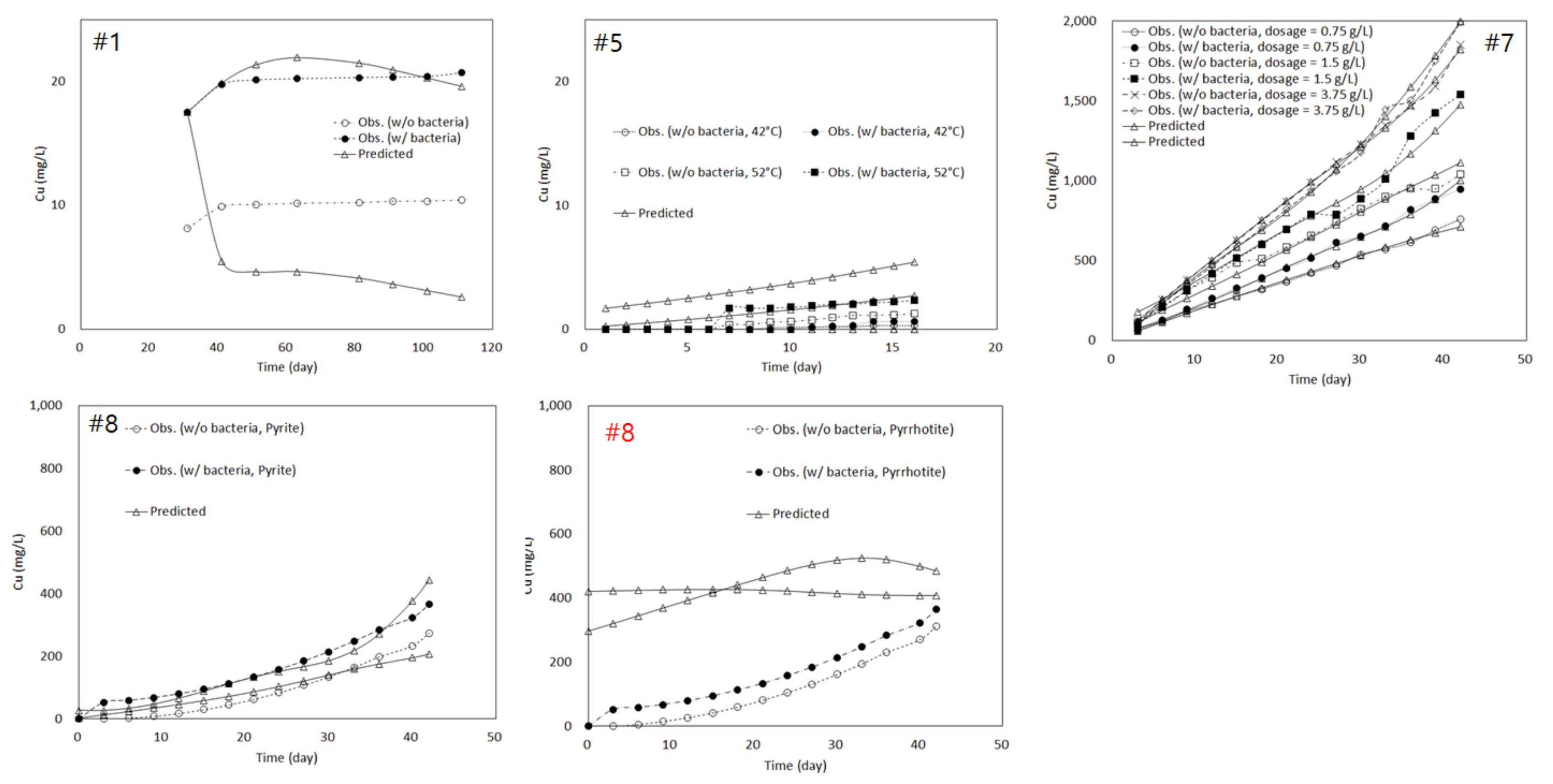
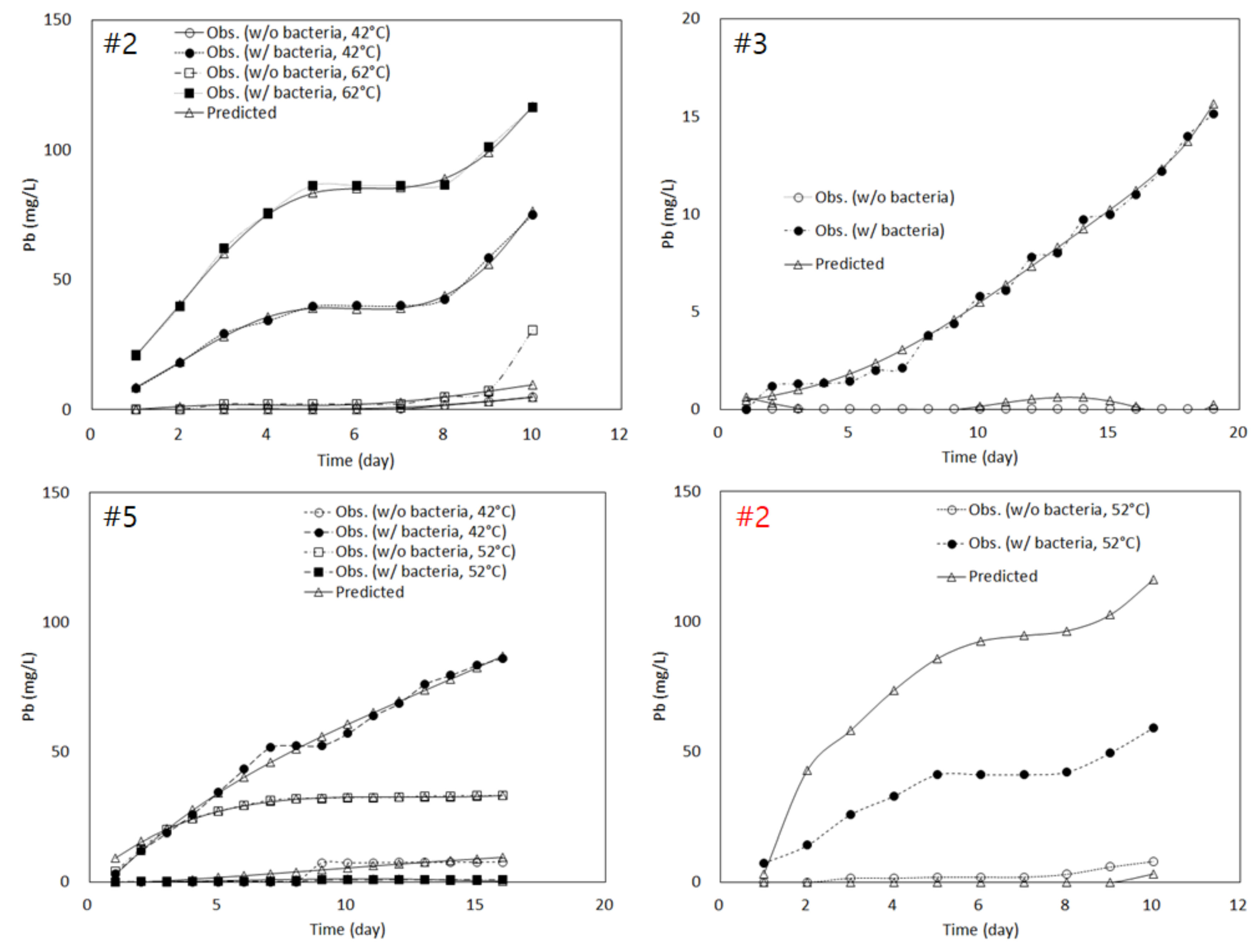
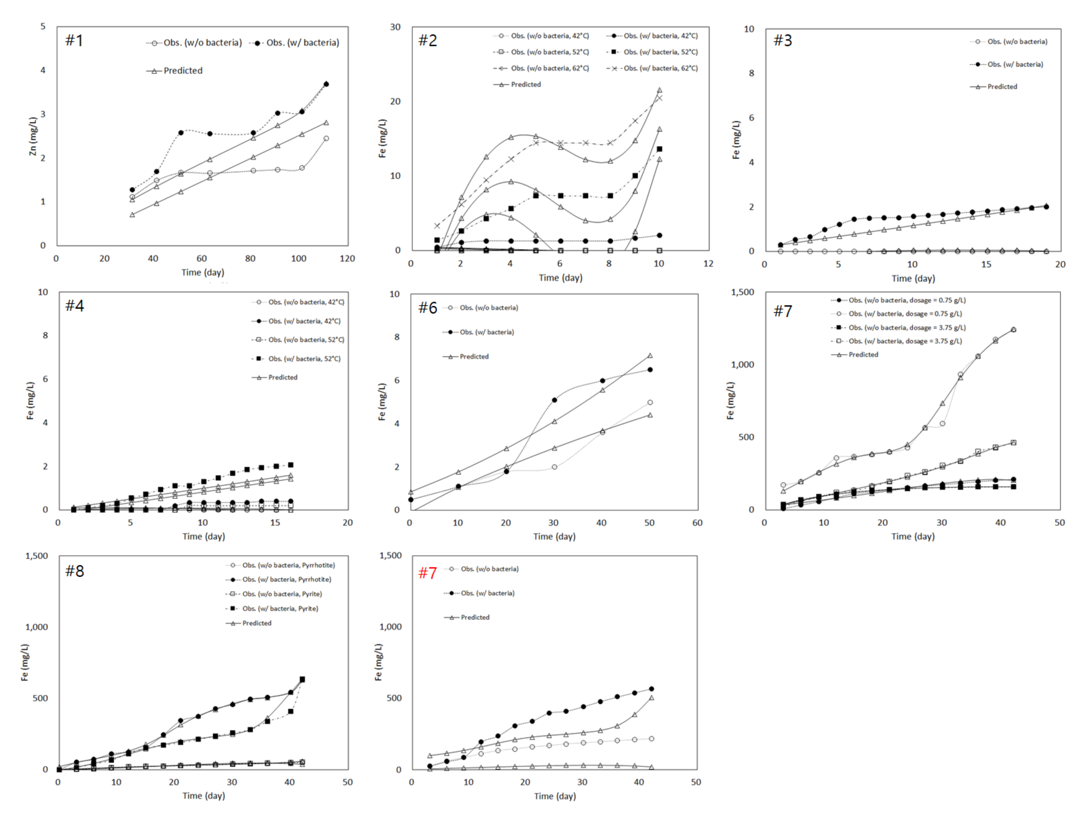
3.2. ANN Modeling for Heavy Metals’ Concentration
4. Conclusions
Author Contributions
Funding
Conflicts of Interest
References
- Vyas, S.; Ting, Y.-P. Sequential biological process for molybdenum extraction from hydrodesulphurization spent catalyst. Chemosphere 2016, 160, 1. [Google Scholar] [CrossRef]
- Vera, M.; Schippers, A.; Sand, W. Progress in bioleaching: Fundamentals and mechanisms of bacterial metal sulfide oxidation—Part A. Appl. Microbiol. Biotechnol. 2013, 97, 7529–7541. [Google Scholar] [CrossRef]
- Yin, S.-H.; Wang, L.-M.; Wu, A.-X.; Chen, X.; Yan, R.-F. Research progress in enhanced bioleaching of copper sulfides under the intervention of microbial communities. Int. J. Miner. Metall. Mater. 2019, 26, 1337–1350. [Google Scholar] [CrossRef]
- Geyikçi, F.; Çoruh, S.; Kılıç, E. Development of Experimental Results by Artificial Neural Network Model for Adsorption of Cu2+ Using Single Wall Carbon Nanotubes. Sep. Sci. Technol. 2013, 48, 1490–1499. [Google Scholar] [CrossRef]
- Aghav, R.M.; Kumar, S.; Mukherjee, S.N. Artificial neural network modeling in competitive adsorption of phenol and resorcinol from water environment using some carbonaceous adsorbents. J. Hazard. Mater. 2011, 188, 67–77. [Google Scholar] [CrossRef] [PubMed]
- Gadekar, M.R.; Ahammed, M.M. Modelling dye removal by adsorption onto water treatment residuals using combined response surface methodology-artificial neural network approach. J. Environ. Manag. 2019, 231, 241–248. [Google Scholar] [CrossRef] [PubMed]
- Ye, J.; Cong, X.; Zhang, P.; Zeng, G.; Hoffmann, E.; Wu, Y.; Zhang, H.; Fang, W. Operational parameter impact and back propagation artificial neural network modeling for phosphate adsorption onto acid-activated neutralized red mud. J. Mol. Liq. 2016, 216, 35–41. [Google Scholar] [CrossRef]
- Laberge, C.; Cluis, D.; Mercier, G. Metal bioleaching prediction in continuous processing of municipal sewage with Thiobacillus ferrooxidans using neural networks. Water Res. 2000, 34, 1145–1156. [Google Scholar] [CrossRef]
- Pazouki, M. Optimizing of Iron Bioleaching from a Contaminated Kaolin Clay by the Use of Artificial Neural Network. Int. J. Eng. 2012, 25, 81–86. [Google Scholar] [CrossRef]
- Abdollahi, H.; Noaparast, M.; Shafaei, S.Z.; Akcil, A.; Panda, S.; Kashi, M.H.; Karimi, P. Prediction and optimization studies for bioleaching of molybdenite concentrate using artificial neural networks and genetic algorithm. Miner. Eng. 2019, 130, 24–35. [Google Scholar] [CrossRef]
- Vyas, S.; Das, S.; Ting, Y.-P. Predictive modeling and response analysis of spent catalyst bioleaching using artificial neural network. Bioresour. Technol. Rep. 2020, 9, 100389. [Google Scholar] [CrossRef]
- Park, C.-Y.; Cheong, K.-H.; Kim, K.-M.; Hong, Y.-U.; Cho, K.-H. Bioleaching of Pyrite from the Abandoned Hwasun Coal Mine Drainage using Indigenous Acidophilic Bacteria. J. Miner. Soc. Korea 2010, 23, 251–265. [Google Scholar]
- Park, C.-Y.; Cheong, K.-H.; Kim, B.-J. The Bioleaching of Sphalerite by Moderately Thermophilic Bacteria. Econ. Environ. Geol. 2010, 43, 573–587. [Google Scholar]
- Park, C.-Y.; Kim, S.-O.; Kim, B.-J. Bioleaching of Galena by Indigenous Bacteria at Room Temperature. J. Miner. Soc. Korea 2010, 23, 331–346. [Google Scholar]
- Park, C.-Y.; Cho, K.-H. The Characteristics of Attachment on Pyrite Surface and Bioleaching by Indigenous Acidophilic Bacteria. J. Korean Soc. Miner. Energy Resour. Eng. 2010, 47, 51–60. [Google Scholar]
- Park, C.-Y.; Cheong, K.-H.; Kim, B.-J.; Wi, H.; Lee, Y.-G. The Corrosion and the Enhance of Bioleaching for Galena by Moderate Thermophilic Indigenous Bacteria. J. Korean Soc. Miner. Energy Resour. Eng. 2011, 59, 11–24. [Google Scholar] [CrossRef]
- Kim, B.-J.; Cho, K.-H.; Choi, N.-C.; Kim, S.-B.; Park, C.-Y. Attachment characteristic of indigenous acidophilic bacteria to pyrite surface in mine waste. Geosyst. Eng. 2012, 15, 123–131. [Google Scholar] [CrossRef]
- Kim, B.-J.; Wi, D.-W.; Choi, N.-C.; Park, C.-Y. The Efficiency of Bioleaching Rates for Valuable Metal Ions from the Mine Waste Ore using the Adapted Indigenous Acidophilic Bacteria with Cu Ion. J. Soil Groundw. Environ. 2012, 17, 9–18. [Google Scholar] [CrossRef] [Green Version]
- Kim, B.-J.; Cho, K.-H.; Choi, N.-C.; Park, C.-Y. The Leaching of Valuable Metal from Mine Waste Rock by the Adaptation Effect and the Direct Oxidation with Indigenous Bacteria. J. Miner. Soc. Korea 2015, 28, 209–220. [Google Scholar] [CrossRef]
- Baziar, M.; Azari, A.; Karimaei, M.; Gupta, V.K.; Agarwal, S.; Sharafi, K.; Maroosi, M.; Shariatifar, N.; Dobaradaran, S. MWCNT-Fe3O4 as a superior adsorbent for microcystins LR removal: Investigation on the magnetic adsorption separation, artificial neural network modeling, and genetic algorithm optimization. J. Mol. Liq. 2017, 241, 102–113. [Google Scholar] [CrossRef]
- Ghaedi, A.M.; Vafaei, A. Applications of artificial neural networks for adsorption removal of dyes from aqueous solution: A review. Adv. Colloid Interface Sci. 2017, 245, 20–39. [Google Scholar] [CrossRef]
- Ma, S.; Tong, L.; Ye, F.; Xiao, J.; Bénard, P.; Chahine, R. Hydrogen purification layered bed optimization based on artificial neural network prediction of breakthrough curves. Int. J. Hydrogen Energy 2019, 44, 5324–5333. [Google Scholar] [CrossRef]


| No.(#) | Reference | Indigenous Acidophilic Bacteria | Cultivation Conditions | Bioleaching Conditions | ||
|---|---|---|---|---|---|---|
| Origin of Bacteria | Temp. (°C) & Cultivation Duration | Adaptation | Temp. (°C) | Sulfide Minerals | ||
| 1 | Park, et al. [12] | Hwasun-gun (Mine drainage) | 32 (21 days) | None adaptation | 32 | Pyrite |
| 2 | Park, et al. [13] | Hatchobaru (Hot spring water) | 32 (21 days) → 42 (21 days), 52 (21 days) or 52 (21 days) → 62 (21 days) | None adaptation | 42, 52, 62 | Sphalerite |
| 3 | Park, et al. [14] | Hatchobaru (Hot spring water) | 32 (21 days) | None adaptation | 32 | Galena |
| 4 | Park and Cho [15] | Hwasun-gun (Mine drainage) | 32 (21 days) | None adaptation | 32 | Pyrite |
| 5 | Park, et al. [16] | Hatchobaru (Hot spring water) | 32 (28 days) → 42 (28 days), 52 (28 days) | None adaptation | 42, 52 | Galena |
| 6 | Kim, et al. [17] | Hatchobaru (Hot spring water) | 32 (21 days) | CuSO4 (5, 10, 25 g/L), 32 ℃ (21 days, 3rd) | 32 | Pyrite |
| 7 | Kim, et al. [18] | Samcheok-si (Mine drainage) | 32 (21 days) | CuSO4 (1.5 g/L), 32 ℃ (21 days, 4th), pH 2.62 | 32 | Pyrrhotite |
| 8 | Kim, et al. [19] | Goseong-gun (Mine drainage) and Younwha (Mine drainage) | 32 (21 days) | CuSO4 (1.5 g/L), 32 ℃ (21 days, 4th), pH 2.82 | 32 | Pyrite, Pyrrhotite |
| # a | Input Variable | Output Variable | ||||||||||||
|---|---|---|---|---|---|---|---|---|---|---|---|---|---|---|
| Origin of Bacteria | Temp. (°C) | Dosage (g/L) | wt. % of Mineral for Energy Source | pH | Eh (mV) | Concentration at Time t (mg/L) | ||||||||
| Pb | Fe | S | Zn | Cu | Cu | Pb | Zn | Fe | ||||||
| 1 | Mine drainage | 32 | 1 | 0 | 45.64 | 50.34 | 0.03 | 0.01 | O | O | O | X | O | O |
| 2 | Hot spring water | 42 | 2 | 3.42 | 0.07 | 9.20 | 87.10 | 0.18 | O | O | X | O | △ | O |
| 52 | O | O | X | △ | O | O | ||||||||
| 62 | O | O | X | O | O | O | ||||||||
| 3 | Hot spring water | 32 | 10 | 13.05 | 0.20 | 39.70 | 46.78 | 0.28 | O | O | X | O | O | O |
| 4 | Mine drainage | 42 | 10 | 0 | 45.64 | 50.34 | 0.03 | 0.01 | O | O, | X | X | O | X |
| 40 | O | △ | X | X | O | X | ||||||||
| 160 | O | O | X | X | O | X | ||||||||
| 5 | Hot spring water | 32 | 10 | 13.05 | 0.20 | 39.70 | 46.78 | 0.28 | O | X | O | O | O | O |
| 6 | Hot spring water | 42 | 10 | 0 | 45.64 | 50.34 | 0.03 | 0.01 | X | X | X | X | O | O |
| 7 | Mine drainage | 32 | 0.75 | 0 | 61.3 | 0 | 28.51 | 10.16 | O | X | O | X | O | O |
| 1.50 | O | X | O | X | O | △ | ||||||||
| 3.75 | O | X | O | X | O | O | ||||||||
| 8 | Mine drainage | 32 | 1.33 | 14.67 | 44.86 | 0 | 6.55 | 33.82 | O | X | △ | X | X | O |
| 1.33 | 0 | 61.3 | 0 | 28.51 | 10.16 | △ | X | O | X | X | O | |||
| Output Variable = pH | Output Variable = Pb Concentration | ||||||||||
|---|---|---|---|---|---|---|---|---|---|---|---|
| Topology | MSE | R | Topology | MSE | R | ||||||
| Training | Validating | Testing | All | Training | Validating | Testing | All | ||||
| 9:5:1 | 1.88 × 10⁻² | 0.98683 | 0.98805 | 0.98824 | 0.98717 | 9:5:1 | 1.19 × 101 | 0.99161 | 0.99194 | 0.94765 | 0.98733 |
| 9:6:1 | 6.63 × 10⁻² | 0.99253 | 0.97083 | 0.97701 | 0.98587 | 9:6:1 | 2.01 × 101 | 0.99640 | 0.98979 | 0.97322 | 0.99022 |
| 9:7:1 | 1.89 × 10⁻² | 0.99388 | 0.98645 | 0.96680 | 0.98880 | 9:7:1 | 2.73 × 101 | 0.99643 | 0.98596 | 0.99625 | 0.99427 |
| 9:8:1 | 4.71 × 10⁻² | 0.98945 | 0.97639 | 0.97344 | 0.98531 | 9:8:1 | 1.03 | 0.99903 | 0.99898 | 0.98709 | 0.99672 |
| 9:9:1 | 1.88 × 10⁻² | 0.98891 | 0.99120 | 0.96851 | 0.98576 | 9:9:1 | 2.57 | 0.98908 | 0.99777 | 0.99561 | 0.99053 |
| 9:10:1 | 8.03 × 10⁻² | 0.98984 | 0.96200 | 0.99112 | 0.98512 | 9:10:1 | 8.28 | 0.99958 | 0.99196 | 0.99664 | 0.99832 |
| 9:11:1 | 3.99 × 10⁻² | 0.99320 | 0.97649 | 0.98098 | 0.98909 | 9:11:1 | 1.34 × 101 | 0.99976 | 0.99129 | 0.96579 | 0.99592 |
| 9:12:1 | 3.49 × 10⁻² | 0.99434 | 0.97890 | 0.86583 | 0.96647 | 9:12:1 | 2.79 | 0.99900 | 0.99850 | 0.99460 | 0.99816 |
| 9:13:1 | 2.30 × 10⁻² | 0.98910 | 0.98815 | 0.98318 | 0.98836 | 9:13:1 | 4.52 | 0.99983 | 0.99410 | 0.96714 | 0.99626 |
| 9:14:1 | 2.71 × 10⁻² | 0.99408 | 0.98046 | 0.97520 | 0.98833 | 9:14:1 | 2.15 × 101 | 0.99196 | 0.99219 | 0.98890 | 0.99112 |
| 9:15:1 | 1.56 × 10⁻² | 0.99166 | 0.99145 | 0.98043 | 0.98933 | 9:15:1 | 4.92 | 0.99953 | 0.99639 | 0.99656 | 0.99898 |
| Output Variable = Eh | Output Variable = Zn Concentration | ||||||||||
| 9:5:1 | 7.50 × 10² | 0.93668 | 0.89680 | 0.93958 | 0.92811 | 9:5:1 | 1.08 × 10² | 0.94053 | 0.95852 | 0.94239 | 0.94096 |
| 9:6:1 | 6.24 × 10² | 0.95502 | 0.90029 | 0.95254 | 0.94887 | 9:6:1 | 1.27 × 10² | 0.97755 | 0.97281 | 0.96433 | 0.97398 |
| 9:7:1 | 3.74 × 10² | 0.96718 | 0.94500 | 0.93575 | 0.95613 | 9:7:1 | 6.24 × 10 | 0.96514 | 0.97332 | 0.91208 | 0.95305 |
| 9:8:1 | 2.48 × 10² | 0.92950 | 0.97255 | 0.93840 | 0.93823 | 9:8:1 | 2.26 × 10² | 0.96537 | 0.95020 | 0.89522 | 0.95181 |
| 9:9:1 | 8.11 × 10² | 0.97031 | 0.88045 | 0.88533 | 0.94309 | 9:9:1 | 4.18 × 10 | 0.99620 | 0.99359 | 0.95409 | 0.99066 |
| 9:10:1 | 1.00 × 10² | 0.95346 | 0.86592 | 0.89387 | 0.92703 | 9:10:1 | 1.65 × 10 | 0.99489 | 0.99689 | 0.99471 | 0.99513 |
| 9:11:1 | 5.82 × 10² | 0.97261 | 0.90556 | 0.90967 | 0.95401 | 9:11:1 | 8.38 × 10 | 0.94072 | 0.98337 | 0.91270 | 0.94649 |
| 9:12:1 | 5.32 × 10² | 0.95631 | 0.91392 | 0.90628 | 0.94656 | 9:12:1 | 9.95 × 10 | 0.99928 | 0.99040 | 0.96825 | 0.99186 |
| 9:13:1 | 3.45 × 10² | 0.95039 | 0.96460 | 0.85625 | 0.93799 | 9:13:1 | 8.40 × 10 | 0.99266 | 0.98798 | 0.94571 | 0.98556 |
| 9:14:1 | 8.22 × 10² | 0.91444 | 0.85820 | 0.88330 | 0.90210 | 9:14:1 | 7.93 × 10 | 0.99881 | 0.97886 | 0.56795 | 0.83919 |
| 9:15:1 | 4.79 × 10² | 0.95758 | 0.93634 | 0.96333 | 0.95560 | 9:15:1 | 4.88 × 10 | 0.99879 | 0.92752 | 0.94511 | 0.98211 |
| Output Variable = Cu Concentration | Output Variable = Fe Concentration | ||||||||||
| 9:5:1 | 3.20 × 10⁴ | 0.92546 | 0.91962 | 0.91324 | 0.92345 | 9:5:1 | 1.54 × 10³ | 0.98483 | 0.98880 | 0.97302 | 0.98450 |
| 9:6:1 | 6.09 × 10² | 0.99919 | 0.99769 | 0.99771 | 0.99873 | 9:6:1 | 5.12 × 10² | 0.99394 | 0.99834 | 0.99204 | 0.99393 |
| 9:7:1 | 4.23 × 10² | 0.99723 | 0.99840 | 0.99861 | 0.99755 | 9:7:1 | 5.91 × 10² | 0.99785 | 0.99203 | 0.98887 | 0.99469 |
| 9:8:1 | 2.79 × 10² | 0.99856 | 0.99898 | 0.99762 | 0.99843 | 9:8:1 | 5.21 × 10² | 0.99581 | 0.99550 | 0.98479 | 0.99254 |
| 9:9:1 | 4.70 × 10² | 0.99892 | 0.99933 | 0.99164 | 0.99824 | 9:9:1 | 2.06 × 10² | 0.99626 | 0.99847 | 0.98752 | 0.99529 |
| 9:10:1 | 5.02 × 10² | 0.99936 | 0.99881 | 0.96353 | 0.99708 | 9:10:1 | 1.61 × 10³ | 0.99595 | 0.98378 | 0.98950 | 0.99237 |
| 9:11:1 | 3.12 × 10² | 0.99965 | 0.99783 | 0.99765 | 0.99925 | 9:11:1 | 1.08 × 10² | 0.99983 | 0.99913 | 0.96762 | 0.99441 |
| 9:12:1 | 4.56 × 10² | 0.99982 | 0.99870 | 0.99670 | 0.99875 | 9:12:1 | 3.87 × 10³ | 0.99936 | 0.98676 | 0.84873 | 0.97653 |
| 9:13:1 | 6.05 × 10² | 0.99972 | 0.99861 | 0.99043 | 0.99877 | 9:13:1 | 3.01 × 10² | 0.99901 | 0.99205 | 0.96456 | 0.99562 |
| 9:14:1 | 1.11 × 10³ | 0.99817 | 0.99797 | 0.99734 | 0.99799 | 9:14:1 | 3.09 × 10² | 0.99707 | 0.99513 | 0.96258 | 0.99359 |
| 9:15:1 | 4.09 × 10² | 0.99967 | 0.99847 | 0.99945 | 0.99950 | 9:15:1 | 2.18 × 10² | 0.99587 | 0.99513 | 0.97344 | 0.99304 |
| k | n | b1,n | b2,n | ||||||||||
|---|---|---|---|---|---|---|---|---|---|---|---|---|---|
| 1 (pH) | 1 | −1.8359 | −0.5773 | 3.4467 | 1.0643 | −0.7742 | 0.7384 | −0.8203 | −0.5840 | 0.2123 | 2.7846 | 1.8333 | −1.1425 |
| 2 | 0.3029 | 0.2556 | 0.3794 | 0.0757 | −0.4440 | 0.2724 | 0.6289 | 1.6562 | −3.2499 | −2.6776 | −1.7529 | ||
| 3 | −0.2106 | −2.2416 | −0.3753 | −0.4279 | −0.7237 | 0.6220 | 0.8634 | −0.7955 | 1.4372 | −1.8043 | 1.2452 | ||
| 4 | −1.6023 | −1.3785 | 0.1525 | −0.6959 | 0.8721 | 0.0333 | −0.8607 | −0.7272 | 1.7346 | 0.7969 | −2.5483 | ||
| 5 | 0.5131 | 0.5832 | 0.3681 | 0.2395 | 1.1243 | −0.2981 | 1.0503 | −0.2049 | 0.7778 | −1.1648 | 1.8170 | ||
| 6 | −1.1223 | −0.2776 | −1.2889 | −0.6451 | 0.1844 | −0.3471 | −0.0171 | −1.0049 | 1.0948 | 0.7656 | −1.3975 | ||
| 7 | 1.2056 | 0.9698 | 0.9130 | 1.7092 | 0.4436 | −1.1965 | 0.5614 | 1.5884 | −3.6822 | −0.1087 | −1.6515 | ||
| 8 | −0.9594 | 0.2545 | −0.1163 | 0.1377 | 1.7136 | −0.8193 | −0.1626 | 0.5510 | −1.6255 | −0.5661 | 1.5122 | ||
| 9 | 0.9223 | −0.3562 | −1.2603 | 0.9949 | −0.9743 | −0.3424 | −0.6378 | 0.2993 | −0.3386 | −0.0620 | 0.8411 | ||
| 10 | 0.5076 | 1.1594 | −0.0768 | −0.7581 | −0.0491 | −1.4832 | −0.7576 | 0.2185 | 1.1602 | 1.0459 | 2.5572 | ||
| 11 | −0.1621 | −0.9027 | 0.6510 | −0.2241 | −0.8159 | −0.5190 | −0.8368 | 1.0646 | 1.4966 | 0.7881 | 0.6699 | ||
| 12 | −0.5456 | −0.1667 | −0.1017 | 0.2104 | −0.9777 | 2.1356 | −1.5266 | −1.5692 | −3.2310 | −1.3250 | 1.9112 | ||
| 13 | 1.0487 | −1.2557 | −0.0252 | −0.7996 | −0.1858 | 0.4946 | −0.8953 | −1.2913 | 2.6020 | −0.4344 | −1.8458 | ||
| 14 | −1.2542 | −0.3957 | 0.0578 | −1.0711 | 1.4680 | −0.6518 | −0.4544 | −0.9984 | −2.3014 | −2.7818 | 1.6115 | ||
| 15 | 1.6246 | −0.9454 | 1.3698 | 1.1486 | −0.4306 | −0.2314 | −1.3949 | −1.2071 | 1.1530 | 3.2805 | 2.4357 | ||
| 2 (Eh) | 1 | −0.9730 | 0.5749 | −0.2938 | −1.2768 | 0.7010 | 0.3428 | 1.1183 | −0.0231 | 2.0385 | −1.1703 | −0.8224 | 0.1266 |
| 2 | 1.8509 | −0.2876 | −0.9761 | −0.1650 | 1.1311 | 0.8280 | −0.3102 | −0.3759 | −0.8201 | −0.6398 | −0.8152 | ||
| 3 | 1.1120 | −1.4866 | 1.3797 | 0.2836 | 0.2823 | −0.3141 | 0.2487 | 1.0354 | 0.3582 | −0.6048 | 0.7924 | ||
| 4 | 0.5821 | 0.4108 | 0.3837 | −0.5084 | −1.2461 | −1.2081 | 0.2052 | −0.2378 | −0.4940 | −0.1794 | −0.8758 | ||
| 5 | 0.8928 | −0.4696 | 0.6497 | 0.2056 | 0.2616 | 1.4350 | −1.1186 | 0.1729 | −0.1506 | −0.1554 | 0.3355 | ||
| 6 | 0.0936 | 1.5361 | −0.5888 | −0.1959 | −0.8125 | 0.2033 | −0.4386 | −0.3422 | 0.5656 | 0.8764 | 1.9108 | ||
| 7 | 0.8116 | 1.6128 | −0.1522 | 0.5207 | 0.8100 | −0.6573 | −0.3160 | −0.4010 | 0.4634 | −1.2549 | 0.8500 | ||
| 8 | 0.7202 | −1.4825 | 1.6523 | −0.2463 | 1.3328 | −0.2157 | −0.4352 | −1.3829 | −2.9691 | 0.6193 | 1.0877 | ||
| 3 (Cu) | 1 | 0.0546 | 2.6183 | −18.433 | 1.6934 | −3.2747 | 4.0627 | −0.8585 | 3.1137 | 0.1861 | −3.4469 | −6.8753 | 1.8638 |
| 2 | 3.0039 | −1.2864 | −6.0271 | −1.2267 | 2.1558 | 1.2980 | −3.0894 | −1.0908 | −0.3851 | −2.3052 | −1.5445 | ||
| 3 | 0.0089 | −0.5823 | 0.1791 | 1.5796 | −0.0264 | 2.1980 | 1.0153 | −3.3129 | 1.3685 | 0.9331 | 6.0830 | ||
| 4 | −0.5762 | 0.2071 | 1.0337 | −0.9460 | 0.9208 | 0.4682 | −2.8878 | 1.4491 | 0.9999 | 1.6439 | 2.4794 | ||
| 5 | 1.2818 | −0.6953 | −0.6416 | −1.4989 | 0.9187 | 0.5235 | −1.6576 | 0.6967 | 0.0258 | −0.4306 | 3.9065 | ||
| 6 | −0.0027 | −1.2121 | −2.1805 | −1.1456 | 0.7809 | −1.2875 | −0.4126 | −1.1862 | 0.0953 | −0.6178 | 2.2103 | ||
| 7 | −1.4457 | 1.3171 | −2.3990 | 1.5757 | −0.9899 | −0.4368 | 2.6398 | −1.2554 | −5.7235 | −2.5273 | 0.1680 | ||
| 8 | 0.0627 | 3.0300 | −10.925 | 2.4852 | −1.4151 | −1.3314 | 0.5520 | 1.3984 | −0.2883 | −4.3651 | 8.9419 | ||
| 4 (Pb) | 1 | −2.8729 | 1.8970 | 0.5522 | 1.4257 | −0.1611 | 1.0143 | −0.4128 | 0.2646 | 0.7227 | 3.0619 | −7.0309 | −3.7447 |
| 2 | 1.0373 | −0.1714 | 0.4947 | −0.3538 | −0.5877 | −1.1983 | 0.2156 | 0.5431 | −0.7291 | −1.9596 | −10.438 | ||
| 3 | 0.5603 | 0.0473 | 1.4111 | −0.3935 | −0.2161 | 0.5175 | −0.8509 | 0.6196 | −1.9838 | 1.0440 | 5.8604 | ||
| 4 | 0.4424 | −0.0247 | 0.8086 | 0.4762 | 0.9451 | 0.6344 | −0.8062 | −0.6208 | −2.4237 | 0.8742 | −3.6743 | ||
| 5 | −0.3870 | −3.4634 | 0.0360 | 1.7278 | 0.3679 | −0.0531 | −1.0728 | −0.1192 | −0.0635 | −0.2032 | −3.1189 | ||
| 6 | −0.2611 | 1.6090 | 1.1576 | 0.0830 | 0.8327 | 0.2223 | −1.1289 | 1.4603 | −0.3974 | −3.0246 | −2.4565 | ||
| 7 | 5.2021 | −10.355 | 0.4791 | −0.6917 | −0.4875 | −0.5713 | −0.1012 | 0.0531 | −0.9278 | −0.7996 | 0.4196 | ||
| 8 | −0.1958 | 7.7520 | 1.8898 | 0.8233 | 2.1443 | 1.2497 | −2.4947 | 2.1704 | −0.2556 | −2.8649 | 3.0570 | ||
| 5 (Zn) | 1 | −10.287 | 0.4657 | −9.3634 | −2.9736 | 5.9524 | 3.8516 | −3.2304 | 1.2372 | 6.6546 | −9.7660 | 4.1320 | 0.2988 |
| 2 | −4.1040 | 0.0291 | −1.8231 | −0.8244 | 2.1629 | 4.1125 | −4.7009 | −0.3972 | −7.0186 | 3.2698 | −7.7731 | ||
| 3 | 3.1161 | −0.0494 | −15.468 | 3.6355 | 1.1733 | 2.0903 | 2.3595 | 3.4897 | −3.3373 | −16.765 | 21.9734 | ||
| 4 | −9.2985 | −1.8445 | −8.5123 | −2.6284 | −5.6654 | 1.4913 | 4.3116 | −8.4520 | 6.2033 | −5.9068 | −2.8550 | ||
| 5 | −20.219 | 0.3632 | −16.453 | −6.9686 | 6.4366 | 7.3022 | −1.9315 | 0.5264 | 7.8346 | −19.280 | −1.2829 | ||
| 6 | 4.3078 | 0.2772 | −47.308 | 5.3583 | −1.7586 | 1.9018 | 6.7815 | 5.8244 | 4.3305 | −37.925 | 3.0210 | ||
| 7 | 5.9236 | −6.6622 | 11.736 | 5.8043 | −1.7915 | −6.5833 | 4.2585 | 6.7263 | 3.9652 | 1.1064 | −3.4844 | ||
| 8 | −3.7780 | 1.9959 | 1.3472 | 1.9934 | −4.0865 | −1.6993 | 3.0945 | 0.6467 | −6.5578 | −4.4887 | −2.6997 | ||
| 9 | −3.2367 | 0.0535 | 17.982 | −2.8123 | −1.0770 | −1.5942 | −2.2231 | −2.8243 | 1.5725 | 18.393 | 27.7257 | ||
| 10 | −0.0006 | 2.2508 | 0.0008 | −0.2874 | 2.3572 | 0.3727 | −1.4831 | 1.9732 | −0.0018 | 1.2361 | −8.1480 | ||
| 6 (Fe) | 1 | −2.0472 | −1.2388 | 0.1890 | −2.9874 | 0.0253 | 1.5880 | −1.5456 | −2.5311 | −11.111 | 3.5008 | −3.6381 | 2.6446 |
| 2 | 11.0687 | −0.6581 | 5.6492 | −0.1175 | 1.5025 | −2.8188 | 1.2293 | 0.4918 | −4.9601 | −1.2841 | −1.7426 | ||
| 3 | 2.3606 | −0.3783 | 7.0444 | 0.7734 | 1.5013 | −0.1337 | −1.2103 | 0.6122 | −1.0504 | 0.9746 | −1.9904 | ||
| 4 | 2.0302 | −0.0790 | 0.9703 | 0.9390 | 0.1281 | 0.4920 | −0.0376 | 0.3373 | −0.5258 | −1.2436 | −0.1028 | ||
| 5 | 1.2617 | −0.0452 | −3.3536 | −0.1879 | 1.6096 | 0.3745 | 1.8760 | 1.3136 | 0.8371 | −3.2707 | 5.5881 | ||
| 6 | −1.6305 | 0.0070 | −0.6385 | −0.2182 | −1.4218 | −0.2961 | 2.4693 | −0.6171 | 0.0455 | −1.1830 | −2.3856 | ||
| 7 | −4.9773 | 0.0535 | 13.271 | 0.1907 | −0.3242 | −1.7288 | −1.6067 | −1.7647 | −8.7920 | 5.4787 | 0.4033 | ||
| 8 | −4.1815 | 0.0695 | −3.7940 | −2.4388 | −0.8110 | −2.6524 | 3.7656 | −0.8399 | 4.3613 | −3.3659 | 0.6112 | ||
| 9 | −4.8301 | −0.0001 | −2.9382 | 1.1483 | 2.3878 | 0.1167 | −0.9756 | −1.4167 | 0.0036 | −4.2760 | −3.9266 | ||
| 10 | 2.0727 | −0.1165 | −2.1945 | −0.5926 | 2.0109 | −0.5462 | 0.3940 | 1.7223 | 1.9980 | −3.4825 | −3.7974 | ||
| 11 | 1.7264 | −0.0061 | −1.5267 | −1.2276 | 0.4093 | −0.4586 | 0.5924 | 0.0399 | −0.0771 | 2.0835 | −0.4942 | ||
Publisher’s Note: MDPI stays neutral with regard to jurisdictional claims in published maps and institutional affiliations. |
© 2020 by the authors. Licensee MDPI, Basel, Switzerland. This article is an open access article distributed under the terms and conditions of the Creative Commons Attribution (CC BY) license (http://creativecommons.org/licenses/by/4.0/).
Share and Cite
Kang, J.-K.; Cho, K.-H.; Kim, S.-B.; Choi, N.-C. Artificial Neural Network Modeling for Prediction of Dynamic Changes in Solution from Bioleaching by Indigenous Acidophilic Bacteria. Appl. Sci. 2020, 10, 7569. https://doi.org/10.3390/app10217569
Kang J-K, Cho K-H, Kim S-B, Choi N-C. Artificial Neural Network Modeling for Prediction of Dynamic Changes in Solution from Bioleaching by Indigenous Acidophilic Bacteria. Applied Sciences. 2020; 10(21):7569. https://doi.org/10.3390/app10217569
Chicago/Turabian StyleKang, Jin-Kyu, Kang-Hee Cho, Song-Bae Kim, and Nag-Choul Choi. 2020. "Artificial Neural Network Modeling for Prediction of Dynamic Changes in Solution from Bioleaching by Indigenous Acidophilic Bacteria" Applied Sciences 10, no. 21: 7569. https://doi.org/10.3390/app10217569