1. Introduction
Wind energy gains strength year after year. This renewable energy is becoming one of the most used clean energies worldwide due to its high efficiency, its competitive payback, and the growth in investment in sustainable policies in many countries [
1]. Despite its recent great development, there are still many engineering challenges regarding wind turbines (WT) technology that must be addressed [
2].
From the control perspective, one of the main goals is to stabilize the output power of the WT around its rated value. This should be achieved while the efficiency is maximized, and vibrations and fatigue are minimized. Even more, safety must be guaranteed under all operation conditions. This may even be more critical for floating offshore wind turbines (FOWT), as it has been proved that the control system can affect the stability of the floating device [
3,
4]. This general and ambitious control objective is implemented in many different control actions, depending on the type of WT. So, the pitch angle control is normally used to maintain the output power close to its rated value once the wind speed overpasses a certain threshold. The control of the generator speed is intended to track the optimum rotor velocity when the wind speed is below the rated output speed. And finally, the yaw angle control is used to optimize the attitude of the nacelle to follow the wind stream direction.
This work is focused on the pitch control of the wind turbine. Blade pitch control technology alters the pitch angle of a blade to change the angle of wind attack and ultimately to change the aerodynamic forces on the blades of a WT. Therefore, this control system pitches the blades usually a few degrees every time the wind changes in order to keep the rotor blades at the required angle, thus controlling the rotational speed of the turbine [
5,
6]. This is not a trivial task due to the non-linearity of the equations that describe its dynamics, the coupling between the internal variables, and uncertainty that comes from external loads [
7], mainly wind and, in the case of FOWT, also waves and currents, that makes its dynamics changes [
8]. The complexity of this system has led to propose the use of advanced and intelligent control techniques such as fuzzy logic, neural networks, and reinforcement learning, among others, to address WT related control problems.
Among control solutions, sliding mode control, and adaptive control have been recently applied to WT with encouraging results. In Liu et al. [
9], a PI-type sliding mode control (SMC) strategy for (permanent magnet synchronous generator) PMSG-based wind energy conversion system (WECS) uncertainties is presented. Nasiri et al. propose a super-twisting sliding mode control for a gearless wind turbine by a permanent magnet synchronous generator [
10]. A robust SMC approach to control the rotor speed in the presence of uncertainties in the model is also proposed in Colombo et al. [
11]. In addition, closed loop convergence of the whole system is proved. In Yin et al. [
12], an adaptive robust integral SMC pitch angle controller and a projection-type adaptation law are synthesized to accurately track the desired pitch angle trajectory, while it compensates model uncertainties and disturbances. Bashetty et al. propose an adaptive controller for pitch and torque control of the wind turbines operating under turbulent wind conditions [
13].
The WT control problem has also been addressed in the literature using different intelligent control techniques, mainly fuzzy logic and neuro-fuzzy inference systems [
14,
15,
16,
17,
18,
19,
20,
21]. Reinforcement learning has been an inspiration for the design of control strategies [
22,
23]. A recent overview of deep reinforcement learning for power system applications can be found in Zhang et al. [
24]. In Fernandez-Gauna et al. [
25], RL is used for the control of variable speed wind turbines. Particularly, it adapts conventional variable speed WT controllers to changing wind conditions. As a further step, the same authors apply conditioned RL (CRL) to this complex control scenario with large state-action spaces to be explored [
26]. In Abouheaf et al. [
27], an online controller based on a policy iteration reinforcement learning paradigm along with an adaptive actor-critic technique is applied to the doubly fed induction generator wind turbines. Sedighizadeh proposes an adaptive PID controller tuned by RL [
28]. An artificial neural network based on RL for WT yaw control is presented in Saénz-Aguirre et al. [
29]. In a more recent paper, the authors propose a performance enhancement of this wind turbine neuro–RL yaw control [
30].
The paper by Kuznetsova proposes a RL algorithm to plan the battery scheduling in order to optimize the use of the grid [
31]. Tomin et al. propose adaptive control techniques, which first extract the stochastic property of wind speed using a trained RL agent, and then apply their obtained optimal policy to the wind turbine adaptive control design [
32]. In Hosseini et al., passive RL solved by particle swarm optimization policy (PSO-P) is used to handle an adaptive neuro-fuzzy inference system type-2 structure with unsupervised clustering for controlling the pitch angle of a real wind turbine [
33]. Chen et al. also propose a robust wind turbine controller that adopts adaptive dynamic programming based on RL and system state data [
34]. In a related problem, deep reinforcement learning with knowledge assisted learning are applied to deal with the wake effect in a cooperative wind farm control [
35].
To summarize, in the literature, the RL approach has been applied to the different control actions of wind turbines or to other related problems with successful results. However, this learning strategy has not been directly applied to the pitch control, neither the reward mechanisms have been analyzed in order to improve the control performance. Thus, in the present work, the RL-inspired pitch control proposed in Sierra-García et al. [
36] has been extended to complete the range of reward policies. Novel reward strategies related to the energy deviation from the rated power, namely Mean Squared Error Reward Strategy (MSE-RS), Mean error Reward Strategy (Mean-RS), and the corresponding increments, ∆MSE-RS and ∆Mean-RS, have been proposed, implemented, and combined.
In addition, many of the previous works based on RL execute ϵ-greedy methods in order to increase the exploration level and avoid actions unexplored. The ϵ-greedy methods select an action either randomly or considering the previous experiences, the latter being called greedy selection. The greedy selection is carried out trying to maximize the future expected rewards, based on the previous rewards already received. The probability of selecting a random action is and the probability of performing a greedy selection is . This approach tends to improve the convergence of the learning, but its main drawback is that it introduces a higher randomness in the process and makes the system less deterministic. To avoid the use of ϵ-greedy methods, the concept of Positive-Negative (P-N) rewards, and its relationship with the exploration-exploitation dilemma is here introduced and linked to the WT control problem. An advantage of P-N rewards, observed in this work, is that the behavior is generally more deterministic than ϵ-greedy, allowing more replicable results with fewer iterations.
Moreover, a deep study of the influence of the type of reward in the performance of the system response and in the learning speed has also been carried out. As it will be shown in the simulation experiments, P-N rewards work better than Only-Positive (O-P) rewards for all the policy update algorithms. However, the combination of P-N with O-P rewards helps to soften the variance of the output power.
The rest of the paper is organized as follows.
Section 2 describes the model of the small wind turbine used.
Section 3 explains the RL-based controller architecture, the policy update algorithms and the reward strategies implemented. The results for different configurations are analyzed and discussed in
Section 4. The paper ends with the conclusions and future works.
2. Wind Turbine Model Description
The model of a small turbine of 7 kW is used. The equations of the model are summarized in Equations (1)–(6). The development of these equations can be found in Sierra-García et al. [
18].
where
is the armature inductance (H),
is a dimensionless constant of the generator,
is the magnetic flow coupling constant (V·s/rad),
is the armature resistance (Ω),
is the resistance of the load (Ω), considered in the study as purely resistive, 𝑤 is the angular rotor speed (rad/s),
is the armature current (A), the values of the coefficients
to
depend on the characteristics of the wind turbine,
is the rotational inertia (kg m
2),
is the radius or blade length (m),
is the air density (kg/m
3),
is wind speed (m/s),
is the friction coefficient (N m/rad/s),
is the reference for the pitch (rad), and
is the pitch (rad).
The state variables of the control system are the current in the armature and the angular speed of the rotor, ]. On the other hand, the manipulated or control input variable is the pitch angle, , and the controlled variable is the output power, , unlike other works where the rotor speed is the controlled variable.
The RL controller proposed in this paper is applied to generate a pitch reference signal, , in order to stabilize the output power, , of the wind turbine around its rated value. Equations (1)–(6) are used to simulate the behavior of the wind turbine and thus allow us to evaluate the performance of the controller.
The values of the parameters used during the simulations (
Table 1) are taken from Mikati et al. [
37].
3. RL-Inspired Controller
The reinforcement learning approach consists of an environment, an agent and an interpreter. The agent, based on the state perceived by the interpreter
and the previous rewards provided by the interpreter
, selects the best action to be carried out. This action,
, produces an effect on the environment. This fact is observed by the interpreter who provides information to the agent about the new state,
, and the reward of the previous action,
, closing the loop [
38,
39]. Some authors consider that the interpreter is embedded in either the environment or the agent; in any case, the function of the interpreter is always present.
Discrete reinforcement learning can be expressed as follows [
40]:
is a finite set of states perceived by the interpreter. This set is made with variables of the environment, which must be observable by the interpreter and may be different to the state variables of the environment.
is a finite set of actions to be conducted by the agent.
is the state at
is the action performed by the agent when the interpreter perceives the state
is the reward received after action is carried out
is the state after action is carried out
The environment or world is a Markov process:
is the policy; this function provides the probability of selection of an action for every pair
is the probability that a state changes from to with action
is the probability of selecting action at state under policy
is the expected one-step reward
is the expected sum of discounted rewards
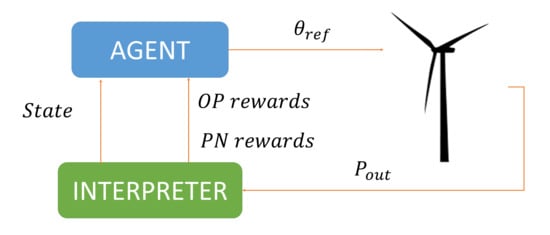
The scheme of the designed controller inspired by this RL approach is presented in
Figure 1. It is composed by a state estimator, a reward calculator, a policy table, an actuator, and a method to update the policy. The state estimator receives the output power error (
,), defined as the difference between the rated power
and the current output power
, and its derivative,
. These signals are discretized and define the state
, where
is the current time. The interpreter is implemented by the state estimator and the reward calculator. The agent includes the policy, the policy update algorithm and the actuator. Both interpreter and agent form the controller (
Figure 1).
The policy is defined as a function which assigns an action to each state in . This action is selected in a way that maximizes the long-term expected reward. The actuator transforms the discrete action into a control signal for the pitch in the range . Each time an action is executed, in the next iteration, the reward calculator observes the new and and calculates a reward/penalty for action . The policy update algorithm uses this reward to modify the policy for the state .
The policy has been implemented as a table together with a function . The table relates each pair with a real number that represents an estimation of the long-term expected reward, that is, the one that will be received when action is executed in the state , also known as . The estimate depends on the policy update algorithm. The table has s rows (states) and a columns (actions). Given a state , the function searches for the action with the maximum value of in the table.
3.1. Policy Update Algorithm
The policy update algorithm calculates the estimate corresponding to the previous pair
of the
each control cycle. At
, the last state and action, that is,
, are updated by the policy function
, using the previous estimation of the long-term expected reward
and the current reward
, Equation (7).
Once the table
is updated, the table is searched for the action that maximizes the reward, Equation (8):
The different policy update algorithms that have been implemented and compared in the experiments are the following
One-reward (OR), the last one received. As it only takes into account the last reward (smallest memory), it may be very useful when the system to be controlled changes frequently, Equation (9)
Summation of all previous rewards (SAR). It may cause an overflow in the long term, that could be solved if the values are saturated to be maintained within some limits, Equation (10)
Mean of all previous rewards (MAR). This policy gives more opportunities to not yet selected actions than SAR, especially when there are many rewards with the same sign, Equation (11)
Only learning with learning rate (OL-LR). It considers a percentage of all previous rewards, Equation (12), given by the learning rate parameter
.
Learning and forgetting with learning rate (LF-LR). The previous methods do not forget any previous reward; this may be effective for steady systems but for changing models it might be advantageous to forget some previous rewards, Equation (13). The forgetting factor is modelled as the complementary leaning rate
.
Q-learning (QL). The discount factor,
is included in the policy function, Equations (14) and (15).
3.2. Exploring Reward Strategies
Once the table and the function are implemented, and a policy update algorithm is selected, it is necessary to define the reward strategy of the reinforcement learning procedure. Although so far the definition of the policy update algorithm is general, the design of the rewards and punishments requires expert knowledge about the specific system.
In this work the target is to stabilize the output power of the WT around it nominal value thus reducing the error between the output power and the rated power. The error will then be the key to define the reward.
3.2.1. Only Positive (O-P) Reward Strategies
The most intuitive approach seems to be rewarding the relative position of the system output to the rated (reference) value. The closer the output to the desired value, the bigger the reward. However, considering the distance (absolute value of the error), the reward grows with the error. To avoid this problem, a maximum error is defined,
, and the absolute error is subtracted from it. This is called “Position Reward Strategy” (PRS), Equation (16).
This strategy only provides positive rewards and no punishments. Thus it belongs to the category only positive (O-P) reinforcement. As it will be seen in the results section, this is the cause of its lack of convergence when individually applied. The main drawback of O-P rewards is that the same actions are selected repeatedly, and many others are not explored. This means that the optimal actions are rarely visited. To solve it, exploration can be externally forced by greedy-methods [
40] or O-P rewards can be combined with positive-negative reinforcement (P-N rewards).
To illustrate the problem, let be initialized to 0 for all the states and actions, . At the system is in the state . Since all actions have the same value in the table, any action is at random selected. At the next control time the state is , which can be different or equal to . The reward received is > 0. The policy update algorithm modifies the value of the table associated to the previous pair (state, action) . Now a new action associated with state must be selected. If the action is randomly selected again because all the actions in the row have the value 0. However, if the state is the same as the previous one, the selected action is the same as in , because is the maximum value of the row. In that case, at the next control time the table is updated . With this O-P rewards this value always tends to be greater than 0, forcing the same actions to be selected. Only some specific QL configurations may give negative values. This process is repeated every control period. If the state action is different from all previous states, a new cell in the table is populated. Otherwise, the selected action will be the first action selected in that state.
If the initialization of the table
is high enough (regarding the rewards), we can ensure that all actions will be visited at least once for OR, MAR and QL update policies. This can be a solution if the system is stationary, because the best action for each state does not change, so that once all the actions have been tested, the optimum one has necessarily been found. However, if the system is changing this method is not enough. In these cases,
-greedy methods have shown successful results [
40]. In each control period, the new action is randomly selected with a probability
(forced exploration) or selected from the table
with a probability (1−
) (exploitation).
Another possible measure that can be used with the O-P strategy to calculate the reward is the previous MSE. In this case, the reward is calculated by applying a time window to capture the errors prior to the current moment. We have called this strategy “MSE reward strategy” (MSE-RS) and it is calculated by Equation (17):
where
is the time length window;
is the variable step size at
, and
is calculated so
. As it may be observed, greater errors will produce smaller rewards.
In a similar way it is possible to use the mean value, “Mean reward strategy” (Mean-RS), that is defined as Equation (18),
In the results section it will be shown how the Mean-RS strategy reduces the mean of the output error and cuts down the error when it is combined with a P-N reward
3.2.2. Positive Negative (P-N) Reward Strategies
Unlike O-P reinforcement, P-N reward strategies encourage the natural exploration of actions that enable convergence of learning. The positive and negative rewards compensate the values of the table , which makes it easier to carry out different actions even if the states are repeated. An advantage of natural exploration over -greedy methods is that their behavior is more deterministic. This provides more repeatable results with fewer iterations. However, the disadvantage is that if rewards are not well balanced, the exploration may be insufficient.
To ensure that the rewards are well balanced, it is helpful to calculate the rewards with some measure of the error variance. PRS, MSE-RS, Mean-RS perform an error measurement in a specific period of time. They do provide neither a measure of the variation nor how quickly its value changes. A natural evolution of PRS is to use speed rather than position to measure whether we are getting closer to or away from rated power and how fast we are doing so. We call it “velocity reward strategy” (VRS), Equations (19) and (20).
The calculation is divided into two parts. First, is calculated to indicate whether we are getting closer to or away from the nominal power, Equation (19). If the error is positive and decreases, we are getting closer to the reference. The second part is to detect when the error changes sign and the new absolute error is less than the previous one. It would be a punished action according to Equation (19) but when this case is detected, the punishment becomes a reward, Equation (20).
A change in the MSE-RS can also be measured as Equation (17). This produces a new P-N reward, the ∆MSE-RS, which is calculated by Equation (21):
Comparing Equation (17) and Equation (21) it is possible to observe how the reward is calculated by subtracting the inverse of MSE-RS at from the inverse of MSE-RS at . In this way, if the MSE is reduced, the reward is positive; otherwise it is negative.
Similar to MSE, a P-N reward strategy can be obtained based on the mean value of the error. It is calculated with Equation (22) and is called
.
As will be shown in the results, the improve the mean value of the error compared to other reward strategies.
In addition to these P-N rewards, it is possible to define new rewards strategies by combining O-P with P-N rewards, such as PRSVRS. However, the combination of P-N rewards between them does not generally provide better results; even in the same cases this combination can produce an effective O-P reward if they always have the same sign.
4. Simulation Results and Discussion
An in-depth analysis of the performance of the RL controller under different configurations and reward strategies has been carried out. The algorithm has been coded by the authors using Matlab/Simulink software. The duration of each simulation is 100 s. To reduce the discretization error, a variable step size has been used for simulations, with a maximum step size of 10 ms. The control sampling period has been set to 100 ms. In all the experiments, the wind speed is randomly generated between 11.5 m/s and 14 m/s.
For comparison purposes, a PID is also designed with the same goal of stabilizing the output power around the rated value of the wind turbine. Thus, the input of the PID regulator is the output power and its output is the pitch angle reference. In order to make a fair comparison, the PID output has been scaled to adjust its range to [0, π/2] rad and it has been also biased by the term π/4. The output of the PID is saturated for values below 0° and above 90°. The parameters of the PID have been tuned by trial and error, and they have been set to KP = 0.9, KD = 0.2 and KI = 0.5.
Figure 2 compares the power output, the generator torque and the pitch signal obtained with different control strategies. The blue line represents the output power when the angle of the blades is 0°, that is, the wind turbine collects the maximum energy from the wind. As you would expect, this action provides maximum power output. The red line represents the opposite case, the pitch angle is set to 90° (feather position). In this position, the blades offer minimal resistance to the wind, so the energy extracted is also minimal. The pitch angle reference values are fixed for the open loop system in both cases, without using any external controller. In a real wind turbine, there is a controller to regulate the current of the blade rotor in order to adjust the pitch angle. In our work this is simulated by Equation (5). The yellow line is the output obtained with the PID, the purple line when the RL controller is used, and the green is the rated power. In this experiment, the policy update algorithm is SAR and the reward strategy is VRS. It is observed how the response of the RL controller is much better than that of the PID, with smaller error and less variation. As expected, the pitch signal is smoother with the PID regulator than with the RL controller. However, as a counterpart, the PID reacts slower, producing bigger overshoot and longer stabilization time of the power output.
Several experiments have been carried out comparing the performance of the RL controller when using different policy update algorithms and reward strategies. The quantitative results are presented in
Table 2,
Table 3 and
Table 4 and confirm the graphical results of
Figure 2. These data were extracted at the end of iteration 25. The reward window was set to 100 ms. In these tables, the best results per column (policy) have been boldfaced and the best results per row (reward) have been underlined.
The smallest MSE error is obtained by combining SAR and VRS. Overall, SAR provides the best results, closely followed by MAR and OL-LR. As expected, the worst results are produced by O-R, this can be explained because it only considers the last reward, which limits the learning capacity. For almost all policy update algorithms, the MSE is lower when VRS is applied; the only exception is QL, which performs better with ∆MSE-RS.
Another interesting result is that the performance of O-P rewards is much worse than for P-N rewards. The reason may be that exploration with O-P rewards is very low, and the best actions for many of the states are not exploited. The exploration can be increased by changing the start of the Qtable. Finally, the P-N reward provides better performance than the PID even with OR.
Table 3 shows the mean value of the power output obtained by these experiments. The best value is obtained by combining OL-LR and ∆MEAN-RS. OL-LR is the best policy update followed by SAR. O-R again provides the worst results. In this case, the best reward strategies are ∆MEAN-RS and ∆MSE-RS. This may be because the mean value measurement is intrinsically considered in the reward calculation.
Table 4 presents the variance of the power output in the previous experiments. Unlike
Table 2, in general, N-P rewards produce worse results than O-P rewards. This is logical because N-P rewards produce more change in the selected actions and a more varying output, therefore more variation. However, it is notable that the combination of VRS and SAR provides a good balance between MSE, mean value, and variance.
Figure 3 represents the evolution of the saturated error and its derivative, iteration by iteration. In this experiment, the combination of SAR and ∆MSE-RS is used. In
Figure 3 it is possible to observe an initial peak of −1000 W in the error (horizontal axis). This error corresponds to an output power of 8 kW (the rate power is 7 kW). It has not been possible to avoid it at the initial stage with any of the tested control strategies, even forcing the pitch to feather. A remarkable result is that, in each iteration, the errors are merged and centered around a cluster. This explains how the mean value of the output power approaches the nominal power over time.
One way to measure the center of this cluster is to use the radius of the centroid of the error calculated by the Equation (23):
Figure 4,
Figure 5,
Figure 6,
Figure 7,
Figure 8 and
Figure 9 show the evolution of the MSE (left) and the error centroid radius (right) for different combinations of reward strategy (
Section 3.2) and policy update algorithm (
Section 3.1). In each figure, the policy update algorithm is the same and a sweep of different reward strategies is performed. Each reward strategy is represented by a different color: PRS in dark blue, VRS in red, MSE-RS in yellow, Mean-RS in purple, ∆MSE-RS in green and ∆MEAN-RS in light blue. It is possible to observe how, in general, the MSE and the radius decrease with time, although the ratio is quite different depending on the combination of policy update algorithm and reward strategy that is used.
The MSE and radius decrease to a minimum, which is typically reached between iterations 5 and 10. The MSE minimum is greater than 260 and is 0 for the radius. The MSE minimum is high because, as explained, the first peak in power output cannot be avoided, it cannot be improved by learning. As expected, the smallest MSE errors correspond to the smallest values of the radius.
Another remarkable result is that iteration by iteration learning is not observed when O-P rewards are applied. This is because, as stated, these strategies do not promote exploration and optimal actions are not discovered. As will be shown in
Section 4.3, this problem is solved when O-P rewards are combined with P-N rewards. It can also be highlighted how all the P-N rewards converge at approximately the same speed up to the minimum value, but this speed is different for each policy update algorithm. From this point on, there are major differences between the P-N reward strategies. For some policy update algorithms (OR, LF-LR, and QL), these differences increase over time, while for the rest, they decrease.
The OR strategy is the one that converges the fastest to the minimum, but from this point, the MSE grows and becomes more unstable. Therefore, it is not recommended in the long term. However, SAR provides a good balance between convergence speed and stability. When it is used, the MSE for the three P-N reward strategies converges to the same value.
As expected, OL-LR and SAR produce very similar results because the only difference between them is that in the former, the rewards are multiplied by a constant. As the rewards are higher, the actions are reinforced more and there are fewer jumps between actions. This can be seen in
Figure 5 and
Figure 7.
4.1. Influence of the Reward Window
Several of the reward strategies calculate the reward applying a time window, that is, considering N previous samples of the error signal, specifically: MSE-RS, MEAN-RS, ∆MSE-RS, ∆MEAN-RS. To evaluate the influence of the size of this window, several experiments have been carried out varying this parameter. In all of them, the policy update algorithm has been SAR.
Figure 10 (left) shows the results when ∆MSE-RS is applied and
Figure 10 (right) for ∆MEAN-RS. Each line is associated with a different window size and is represented in a different color. The reward is a dimensionless parameter as table
is dimensionless. The legend shows the size of the window in seconds. The value −1 indicates that all the previous values, from instant 0 of the simulation, have been taken into account to obtain the reward. That is, the size of the window is variable and increases in each control period, and covers from the start of the simulation to the current moment. MSE-RS and MEAN-RS have not been included as, as explained, they are O-P reward strategies and do not converge without forced exploration.
In general, a small window size results in a faster convergence to the minimum, but if the size is too small it can cause oscillations after the absolute minimum. This happens with a window of 0.01s, the MSE oscillates and is even less stable for ∆MEAN-RS. A small window size produces noisy rewards. This parameter seems to be related to the control period; a size smaller than the control period produces oscillations.
For the ∆MSE-RS strategy, the convergence speed decreases with the size of the window up to 1 s. For smaller window sizes it does not converge. This can be explained as if the window is longer than the control period, the window can be divided into two parts: the value of a control period preceding the end of the
Tw2 window, and the remaining part from the beginning of the
Tw1 window (
Figure 11). An action performed at
produces an effect that is evaluated when the reward is calculated at
. When the size of the window grows during the control period, the
Tw1 part also grows, but
Tw2 remains invariant. To produce positive rewards, it is necessary to reduce the MSE, therefore, during
Tw2, the increases in
Tw1 should be compensated. A larger
Tw1 would give a larger accumulated error in this part, which would be more difficult to compensate during
Tw2 since only the squared error can be positive. It can then be concluded that the optimal window size for ∆MSE-RS is the control period, in this case, 100 ms.
The behavior of ∆MEAN-RS with respect to the size of the window is similar up to a size of around 20 s; from this value increasing the window size accelerates the convergence and decreases the MSE. This is because a larger window size implies a longer
Tw1 part (
Figure 11). However, unlike ∆MSE-RS, a longer
Tw1 produces less accumulated error in
Tw1 since, in this case, the positive errors compensate for the negative ones, and the accumulated error tends to 0. Therefore,
Tw2 has a greater influence on the window, and learning is faster.
Figure 12 shows the variation of the MSE with the size of the reward window, at iteration 5. It is possible to observe how the MSE grows until the size of the window is 1 s, decreases until a size around 10 s, and then it grows again until around 25 s, which continues to grow for ∆MSE-RS and decreases for ∆MEAN-RS. The numerical values of these local minima and maxima are related to the duration of the initial peak (
Figure 2). The O-P rewards have also been represented with different reward windows. It is possible to observe how for long windows, the ∆MSE-RS tends to behave like the O-P reward strategies and reaches the same values.
4.2. Influence of the Size of the Reward
Up to this subsection, the reward mechanism provides a variable size reward/punishment depending on how good the previous action was. Better/worse actions give greater positive/negative rewards. In this section the case of all rewards and punishments having the same size is analyzed. To do so, the P-N reward strategies are binarized, that is, the value +r is assigned if the reward is positive and -r if it is negative. Several experiments have been carried out varying this parameter r to check its influence. In all experiments the policy update algorithm is SAR and the window size is 100 ms.
The results are shown in
Figure 13,
Figure 14 and
Figure 15, on the left the evolution of the MSE and on the right the evolution of the variance. Each line represents a different size of reward with a color code. The legend indicates the size of the reward. “Var” indicates that the reward strategy is not binarized and therefore the size of the reward is variable.
It can be seen how, in all cases, the MSE is much better when the size of the reward is not binarized. However, the variation is similar or even worse. It has already been explained how better MSE performance typically leads to greater variance. Another interesting result is that the speed of convergence does not depend on the size of the reward, all the curves provide similar results up to the absolute minimum. However, from this point on, oscillations appear in the MSE and vary with size.
The VSE reward strategy is the least susceptible to variations in reward size. For ∆MSE-RS, the oscillations seem to depend on the size of the reward: the larger the size, the greater the oscillations; however, its amplitude decreases with time. For ∆MEAN-RS this relationship is not so clear and, what is worse, the amplitude of the oscillations seems to increase with time. Therefore, it is not recommended to use a fixed reward size with ∆MSE-RS and ∆MEAN-RS, it is preferable to use a variable reward size.
4.3. Combination of Individual Reward Strategies
As discussed above, O-P reward strategies do not converge due to the lack of exploration of the entire space of possible actions. To solve this, ϵ-greedy methods can be applied [
40] or they can be combined with P-N reward strategies. This last option is explored in this section. Different experiments have been carried out combining reward strategies O-P with P-N and their performance is studied. In all experiments, the policy update algorithm is SAR and the window size is 100 ms.
Figure 16 shows the results of applying PRS (blue) and VRS (red), PRS
VRS (yellow) and PRS+K
VRS (purple), with K = 2. It is possible to see how the multiplication makes PRS converge. However, this is not true with addition, as this operator cannot convert PRS to a P-N reward strategy in all cases. It depends on the size of each individual reward and on the value of K. Therefore, the addition operator will not be used from now on to combine the rewards. Another interesting result is that the PRS
VRS combination smoothens the VRS curve, the result converges at a slightly slower speed but is more stable for iterations over 15. This combination presents less variance than VRS in general.
Figure 17 shows the results of MSE-RS (blue), MEAN-RS (red), MSE-RS
VRS (yellow), Mean-RS
VRS (purple), and VRS (green). All strategies combined converge at roughly the same speed, slightly slower than VRS. During iteration 10, the performance of VRS and MSE-RS
VRS is similar; however, Mean-RS
VRS worsens its performance over VRS.
In the following experiment, the P-N ∆MSE-RS reward strategy is combined with each O-P reward strategy.
Figure 18 shows the results, PRS (dark blue), MSE-RS (red), ∆MSE-RS (purple), PRS
∆MSE-RS (green), MSE-RS
∆MSE-RS (light blue) and Mean-RS
∆MSE-RS (magenta). Again it is possible to observe how all the combined strategies and ∆MSE-RS converge at the same speed until iteration 5. From this point on ∆MSE-RS and PRS
∆MSE-RS give smaller error MSE. On the other hand, the variance decreases until iteration 5, after which it grows, although less for MSE-RS
∆MSE-RS and Mean-RS
∆MSE-RS. Furthermore, PRS
∆MSE-RS tends to be slightly smaller than ∆MSE-RS.
In this last experiment, the P-N ∆Mean-RS strategy is combined with each O-P strategy.
Figure 19 shows the results, with PRS (dark blue), MSE-RS (red), ∆Mean-RS (purple), PRS
∆Mean-RS (green), Mean-RS
∆MSE-RS (light blue) and Mean-RS
∆Mean-RS (magenta). Again it is possible to observe how all the combined strategies and ∆Mean-RS converge at the same speed until approximately iteration 5, where PRS
∆Mean-RS improves the MSE. The combination of these strategies provides a better result than their individual application. Furthermore, the variance also decreases with iterations. The combination of ∆Mean-RS with Mean-RS and MSE-RS only offers an appreciable improvement in variance.
Table 5 compiles the numerical results of the previous experiments. The KPIs have been measured at iteration 25. The best MSE is obtained by the combination of PRS
VRS and the best mean value and variance by MSE-RS
∆MSE-RS. In general, it is possible to observe how the combination with PRS decreases the MSE and the combination with MEAN-RS and MSE-RS improves the mean value and the variance.
In view of these results, it is possible to conclude that the combination of individual rewards of O-P and P-N is beneficial since it converges learning by O-P rewards, without worsening the speed of convergence and learning is more stable.
5. Conclusions and Future Works
In this work, a RL-inspired pitch control strategy of a wind turbine is presented. The controller is composed by a state estimator, a policy update algorithm, a reward strategy, and an actuator. The reward strategies are specifically designed to consider the energy deviation from the rated power aiming to improve the efficiency of the WT.
The performance of the controller has been tested in simulation on a 7 kW wind turbine model with varying different configuration parameters, especially those related to rewards. The RL-inspired controller performance is compared to a tuned PID giving better results in terms of system response.
The relationship of the rewards with the exploration-exploitation dilemma and the-greedy methods is studied. On this basis, two novel categories of reward strategies are proposed, O-P (Only-Positive) and P-N (Positive-Negative) rewards. The performance of the controller has been analyzed for different reward strategies and different policy update algorithms. The individual behavior of these methods and their combination have also been studied. It has been shown that the P-N rewards improve the learning convergence and the performance of the controller.
The influence of the control parameters and RL configuration on the turbine response has been throughout analyzed and different conclusions regarding learning speed and convergence have been drawn. It is worth noting the relationship between the size of the reward and the need for forced exploration for the convergence of learning.
Some potential challenges may include to extend this proposal to design model-free general purpose tracking controllers. Another research line would be to incorporate risk detection in the P-N reward mechanisms to perform safe non-forced exploration for systems, which must fulfill safety requirements during the learning process.
As other future works, it would be desirable to test the proposal in a real prototype of a wind turbine. Also, it would be interesting to apply this control strategy to a larger turbine, and see if this control action affects the stability of a floating offshore wind turbine.


