Artificial Intelligence for the Prediction of Exhaust Back Pressure Effect on the Performance of Diesel Engines

Featured Application

This paper presents solutions for smart devices with embedded artificial intelligence dedicated to vehicular applications. Virtual sensors based on neural networks or regressors provide real-time predictions on diesel engine power loss caused by increased exhaust back pressure.

Abstract

The actual trade-off among engine emissions and performance requires detailed investigations into exhaust system configurations. Correlations among engine data acquired by sensors are susceptible to artificial intelligence (AI)-driven performance assessment. The influence of exhaust back pressure (EBP) on engine performance, mainly on effective power, was investigated on a turbocharged diesel engine tested on an instrumented dynamometric test-bench. The EBP was externally applied at steady state operation modes defined by speed and load. A complete dataset was collected to supply the statistical analysis and machine learning phases—the training and testing of all the AI solutions developed in order to predict the effective power. By extending the cloud-/edge-computing model with the cloud AI/edge AI paradigm, comprehensive research was conducted on the algorithms and software frameworks most suited to vehicular smart devices. A selection of artificial neural networks (ANNs) and regressors was implemented and evaluated. Two proof-of concept smart devices were built using state-of-the-art technology—one with hardware acceleration for “complete cycle” AI and the other with a compact code and size (“AI in a nut-shell”) with ANN coefficients embedded in the code and occasionally offline “statistical re-calibration”.

1. Introduction

Nowadays, diesel engines are the prime movers in commercial transportation, power generation, and off-road applications. Their major advantages compared to other common alternatives are a better fuel economy, a lower carbon footprint, and an increased reliability. The demands on engine performance indicators—increased power output, lower fuel consumption, and emissions—require a better understanding of engine processes, further experimental investigations, and the implementation of control strategies based on numerical models.

In four-stroke engines, the process of gas exchange requires a very rapid and total release of exhaust gas from cylinders into the atmosphere, which is evaluated by exhaust back pressure (EBP), a flow resistance indicator on the exhaust duct. Unsteady friction and inertial forces, which are dependent on gas velocity, shape, and dimensions of the passages, occur. EBP is defined as the gauge pressure at the turbine outlet for turbocharged engines or at the exhaust manifold outlet for naturally aspirated engines [1].

Diesel engine control based on numerical models tends to become more complicated as the number of independent variables increases, so multidimensional, flexible, and adaptive add-ons based on artificial intelligence (AI) are required; these systems are able to learn from experiments, solve non-linear problems, use scarce data, and predict phenomena.

To the knowledge of the authors, among the high number of articles studying the artificial neural network (ANN) prediction of diesel engine performance, there have been a lack of studies with EBP as an input parameter.

Therefore, the goal of this work was to provide a better understanding of EBP effects on diesel engine parameters, at different loads and speeds, based on engine experiments and AI simulations in order to assess the reasonable performance loss (expressed mainly in power loss) caused by the emission and noise abatement devices.

The main contribution of the paper is the AI application in the interpretation of exhaust pressure loss consequences; the added value of such an approach is the possibility to assess performance decline by means of virtual sensors implemented on smart devices.

The opportunity of the applied research was given by recent progress in cost-effective embedded systems with local processing, storage, and communication capabilities that enable the edge-computing/cloud-computing paradigm of the IoT (the Internet of Things). Centimeter-scale smart devices built around a small SoC (system on chip) IC (integrated circuit) with a WiFi and/or a BLE (Bluetooth Low Energy) radio interface for NFC (near field communications) and a PCB (printed circuit board) antenna are now able to acquire sensor signals via integrated ADCs (analog-to-digital converters). Local signal conditioning and lower/medium complexity processing are performed and results are “published” in the cloud in real-time. These CPS (cyber–physical systems)—the so called “smart dust”/“radio dust”—can also receive cloud directives and download data flows because they are fast-enough for “cyber-critical communications” with time constants much smaller than industrial ones, particularly than vehicular ones. Internet protocols drive IoT WSAN (wireless sensors and actuator networks) that build a pervasive communication eco-system for a test-bench and even for vehicular add-ons to traditional CANs (computer area networks)/device nets on-board. The software subsystems of these compact smart devices are also shrunken down to mini-programs that reside in flash, non-volatile memory chips. Such firmware is built in a low scale IDE (integrated development environment), e.g., Arduino™.

The actual efforts to embed AI in smart devices are discussed from the cloud computing/edge computing perspective.

In terms of methods and apparatus, the study of the EBP effect on diesel engine performance needed a test-bench with appropriate sensors and instrumentation. The setup of data structures for AI-based calculation was followed by database preparation for ANN training and testing. AI for vehicular smart devices was implemented in finite state machine models in an approach similar to object-oriented programming (OOP). ANNs were detailed in the perspective of computational needs for cloud AI versus edge AI. The main ANN training algorithm was SGD (stochastic gradient descent) for BP (back propagation) optimization. The cloud AI implementations were based on MathWorks MATLAB online (with MaaS (Model as a Service) being the optimal choice of Gaussian regressor), the Tensorflow backend (with two APIs (application programming interfaces)—Keras and eXtended Gradient Boosting (XGBoost)) and the ANS Center ANNHUB (for a Levenberg–Marquardt algorithm implementation). Activation functions were mainly ”ReLU” (rectified linear unit) and ”tanh” (hyperbolic tangent), along with the latter’s shift and scaled version: the “sigmoid”. The edge AI high-performance solution with the hardware acceleration of AI computations was based on the NVIDIA Jetson Nano mini-system built around the “Maxwell” SOM (system on module) produced by NVIDIA. The very compact edge AI solution was based on the “TTGO” micro-system produced by LILYGO, centered on the “ESP32” SoC (system on chip) produced by Espressif. As all solutions shared the common complete dataset collected on the engine experimental bench, a separate test flow was implemented via National Instruments LabVIEW virtual instrumentation.

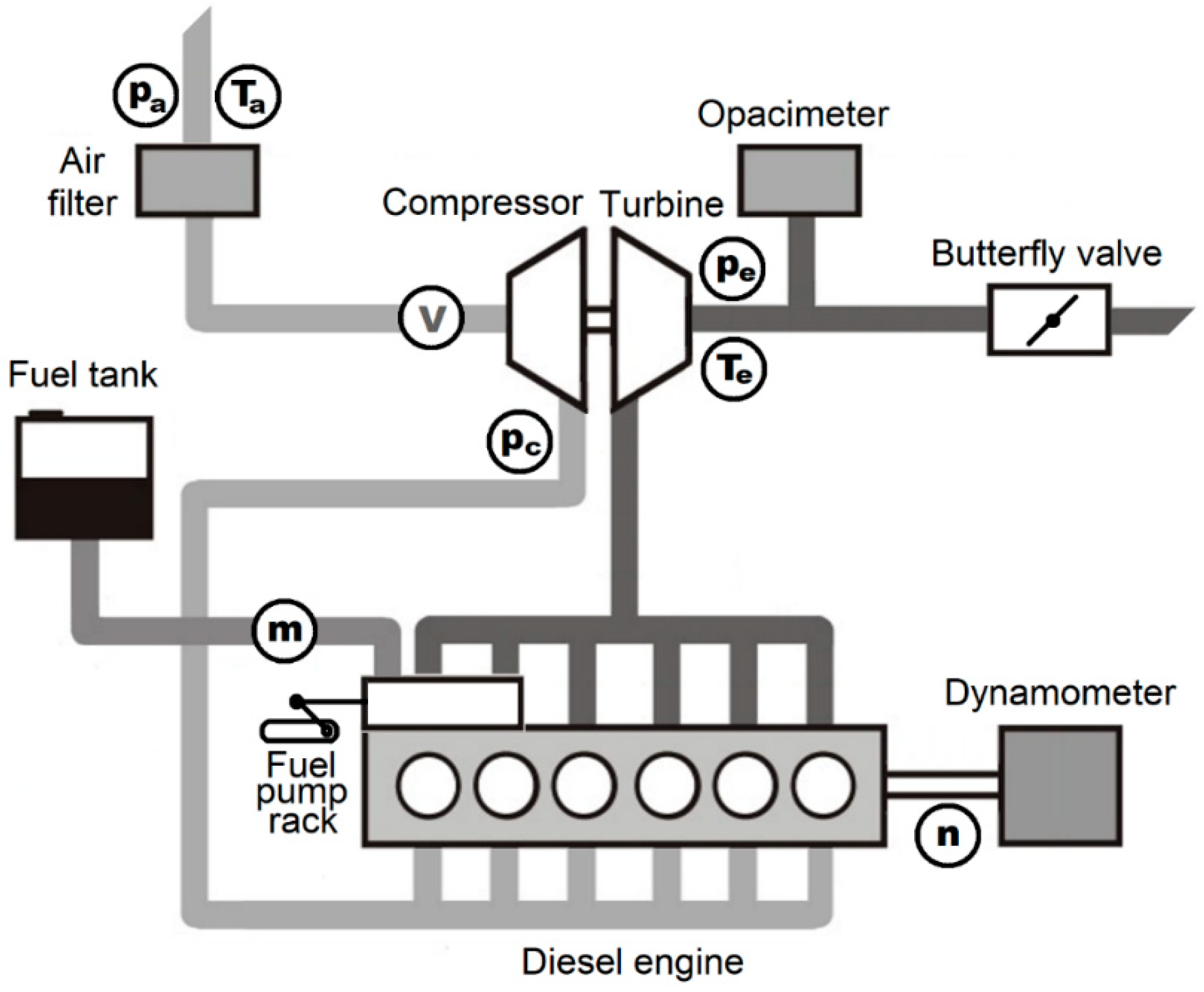
The paper is organized as follows: After the Introduction in Section 1, Section 2 details the related work in the area of EBP and ANN diesel engine optimizations, Section 3 describes the diesel engine experiments performed on the dynamometric test-bench, detailing engine characteristics, instrumentation, and operation mode procedures, as well as complete data collection. Section 4 introduces the AI for the needs of vehicular smart devices, particularly for sensor data processing—the local/centralized placing of AI in a distributed computational environment and AI algorithms applicable to virtual sensors (mainly ANN and classification trees with linear regression branches). Section 5 is dedicated to cloud AI implementations—via MATLAB online, the specific APIs (application programming interfaces) like Keras for ANN, XGBoost (eXtended Gradient Boosting), and the ANNHUB (for an efficient Levenberg–Marquardt implementation). Section 6 is dedicated to the concrete implementations for edge AI, the first one to promote a maximum of miniaturization (minimal code running in an extremely compact hardware) and the second one to promote the maximum of local performance (with hardware acceleration of the AI computation). Section 7 is an interpretation of the results with a testing and performance assessment, Section 8 is a discussion on practical issues, alternatives, usability, and sustainability. Finally, Section 9 presents the main conclusions of the paper.

2. Related Works

This section covers EBP investigations, mainly regarding AI-based predictions in diesel engines and vehicular energy systems. Engine performance is negatively influenced by excessive EBP, thus requiring a higher pumping work to release exhaust gas. The literature has indicated slight reduction of power output and an increase of fuel consumption, exhaust temperature, and smoke emissions. In turbocharged engines, higher EBP means higher turbine outlet pressure, which decelerates the turbocharger, limits the air mass flowrate aspirated in the compressor, and enriches the air–fuel mixture [2,3]. Among engine after-treatment technologies, active DPF (Diesel Particulate Filter) is the most demanding device in terms of pressure drop exigence, and it is thus of paramount importance in the triggering of thermal regeneration process [4].

There are rather few published papers with experimental measures of EBP. For naturally aspirated single-cylinder diesel engines, EBP has been varied in the range of 1.1–1.5 bar, which explains the influence on residual gas fraction and emissions [5,6]; meanwhile, other work [7] has reported increased smoke and a drop of brake thermal efficiency at low loads.

For turbocharged engines, a six-cylinder aftercooled 500 kW diesel engine has been investigated at a constant speed, and the influence of EBP on brake-specific fuel consumption (BSFC), exhaust gas temperature, and emissions was interpreted [8]. Similarly, the testing of a 63 kW turbocharged and intercooled diesel engine at a high EBP impeded engine power, torque, and smoke opacity, reporting, at full load, a drop of power of 9% at an externally applied EBP restriction of 35% out of exhaust duct free section [9].

Accurate EBP measurement is time-consuming and costly, being impeded by pulsing flow and high temperatures; that is why the influence of EBP increase has been frequently investigated with numerical simulation models [5,10]. The exhaust system has been considered a fixed-geometry restriction between the exhaust manifold and the outlet of the tailpipe being implemented a mean-value model to estimate the exhaust manifold pressure from a compressible flow equation. Simulations with Ricardo wave software on a 11-liter submarine diesel engine indicated the reduction of mass flow of air, increased brake-specific fuel consumption, and increased exhaust temperature [3].

Emission abatement techniques such as exhaust gas recirculation (EGR) can be controlled by the accurate estimation of EGR mass flowrate, which requires the engine exhaust pressure as input data. Instead of a physical sensor, virtual sensors are preferred, but their calibration needs real measurements; for example, the research work of [11] reported a virtual sensor, a model-based exhaust manifold pressure estimator that was calibrated with real measurements on a four-cylinder, 1.6 liter turbocharged diesel engine. Similarly, an exhaust pressure estimator was implemented on a 4.9 liter turbocharged and intercooled diesel engine fitted with DPF and DOC (Diesel Oxidation Catalyst) that was calibrated with a physical exhaust pressure sensor for DPF failure detection [12].

An extension of the numerical models for diesel engine study, in terms of number of parameters and processing capabilities, is related to the use of AI methodologies. The most spread AI technique applied to combustion engines is an artificial neural network (ANN). An ANN is a black-box identification technique that is able to automatically learn from examples and to derive models from experimental data. Initially, output and input variables are connected through unknown relations that can be predicted by ANN after training and testing stages [13,14].

Many studies using ANNs in the diesel engine field have been reported, starting from two decades ago; output variables include power [15], torque [16,17], mean effective pressure [15], brake-specific fuel consumption (BSFC) [16,18,19,20], brake thermal efficiency [21,22], cylinder pressure [21], cylinder temperature [23], exhaust gas temperature [16,18,22], emissions [17,21,22,24,25], and mixture/injection parameters (fuel air equivalence ratio [18], maximum injection pressure, and fuel flow rates [21]).

Besides the most widely-used input parameters of engine speed and load, studies have reported power [19], torque [26], fuel injection parameters [19,22,24], cooling fluid temperature [18], fuel properties [27], biodiesel blend [21,22], and compression ratio [22].

New AI techniques have been developed in order to optimize engine operation in the context of vehicular energy systems. Among them, deep reinforced learning (DRL) has demonstrated a fair balance over conflicting objectives, accelerated convergence, and continuous control when applied to fuel economy [28] and battery energy management implemented on hybrid vehicles [29,30].

The aforementioned ANN studies have not considered the influence of EBP on engine parameters, so one of the novelties of this study is related to the investigation of the best approach for implementing AI algorithms working as virtual sensors.

3. Engine Investigations

3.1. Test Facilities and Procedures

The effect of back pressure on engine performance parameters was carried out experimentally on a 1035-L6-DT series commercial vehicle diesel engine manufactured by the Roman truck company; the main characteristics of this engine are given in

Table 1. Engine technical data.

Characteristic	Value
Type	Diesel, 4-stroke, turbocharged, direct injection
Cylinder configuration	6-cylinder, in line
Bore × stroke [mm]	121 × 150
Compression ratio	16:1
Rated power [kW]	172
Rated speed [rpm]	2200
Maximum torque [N·m]	900
Maximum torque speed [rpm]	1600

.

The engine performance was measured in the Engine Testing Laboratory of the Road Vehicle Institute, Brasov on a DC 300 kW/3000 rpm dynamometric test-bench produced by MEZ-Vsetin. The engine layout and the positions of the relevant sensors are illustrated in Figure 1. The bench was instrumented with temperature sensors for exhaust gas, air and cooling fluid, pressure sensors for charge air, ambient air, oil pressure and EBP, flowmeters for air and fuel, a tachometer for engine rotational speed, and an exhaust gas opacimeter. The engine load was adjusted by the fuel control system, and the speed was adjusted by the dynamometer. The EBP was externally applied by a mechanical throttle valve installed on the exhaust system of the test-bench, 2 m downstream the turbine. The adjustment of the EBP was performed manually with intermediate positions calibrated after the maximum EBP values were fixed at rated speed and full load. The exhaust gas temperature was measured using a K-type thermocouple (chromel–alumel) inserted in the exhaust gas duct by means of a bayonet coupling.

The air flow rate was measured by a laminar flow MERIAM flowmeter, the fuel flow rate was measured with a fuel balance produced by AVL List, using the chrono-gravimetric method by measuring the time required to consume 0.5 kg of fuel in any steady point. A digital inductive tachometer was used to read engine speed. The exhaust gas and charged air pressures were read on a Hg U-type manometer and piezo-resistive transducers. In addition to the measurement of engine performance characteristics, the smoke opacity was measured with a Hartridge Dismoke 435 opacimeter produced by AVL List that has an effective length of measurement tube of 430 mm, the readings are expressed both in HSU (Hartridge Smoke Unit) and light absorption coefficients (m⁻¹).

All the instruments met the accuracies imposed by engine testing standard given in Appendix A,

Table A1. Measurement accuracies and result uncertainties.

Measure	Unit	Accuracy
Torque	Nm	±1%
Speed	rpm	±2
Temperature	K	±1
Pressure	kPa	±0.01
Time	s	±0.1
Calculated results	Unit	Uncertainties
Power	kW	±1.1%
Hourly fuel consumption	kg/h	± 0.2%

, along with calculated measure uncertainties. For this engine type, the load was correlated with injection fuel flow, which was adjusted by changing the position of the fuel pump rack. No after-treatment device was mounted on the exhaust duct, as the effect of such was simulated by externally-induced back pressure. Each test started after the engine was warmed up and included a full load and part load tests at rated engine speed with the fuel pump rack fully opened. There were an additional six tests aiming to find part-load curves at intermediate positions of the fuel pump rack. After warming-up, at each set point, the engine was run for 6 min to reach the steady state condition. The experiments were triplicated and averaged to get more accurate values.

A test matrix of 42 distinct operation modes (7 speeds and 6 loads) were chosen to provide a wide range of engine performance map. The speed was adjusted from 1000 to 2200 rpm in 200 rpm increments; the load was set to 100% (full load) and part loads of 90%, 70%, 58%, 48%, and 30%.

In their engine specifications, vehicle manufacturers declare an allowable EBP at which their engine operates and which should not be exceeded. For the tested engine, this limit is 500 mm water column (WC) or 4.9 kPa; as a result, during the test, the minimum value of the externally applied EBP was set to 500 mmWC, and this was considered the reference. The maximum value of the backpressure was set to 3000 mmWC or 29.43 kPa, six times higher than the reference value. Six steps of exhaust back pressure were adjusted from 500 to 3000 mmWC in steps of 500 mmWC for each distinct speed-load combination.

The six EBPs values were adjusted for the engine rated speed of 2200 rpm and full load; lower EBPs resulted in lower engine speeds and loads. Finally, for each of 42 distinct engine operation modes, 6 steps of simulated exhaust back pressure were applied, resulting 42 × 6 = 252 points. For the smallest load (30%) and the highest exhaust back pressure (3000 mmWC), the measurement of parameters at all the seven speeds was not possible due to the construction of the exhaust throttle valve, so the number of operation points was 246.

3.2. Test-Bench Data Analysis

The investigated engine performance parameters included effective power, exhaust gas temperature, brake-specific fuel consumption, boost pressure, and smoke opacity. In the context of this paper, the effective power is thoroughly analyzed, while for the rest of the parameters, there are more qualitative considerations. The influence of EBP upon power, illustrated in Figure 2, was evaluated as a function of load and speed to cover a broad area of engine operation modes.

The profile of the curves indicates the complexity of the dependencies among variables that foresee the need for the latest numerical analysis. For a full load, the relative power loss varied with increasing speed from 0.41% (1000 rpm) to 3.62% (2200 rpm). At the intermediate load of 58%, the variation of the relative power ranged from 2.57% (1000 rpm) to 6.34% (2200 rpm); for the further reduction of the load to 30%, the corresponding figures grew to 5.52% (1000 rpm) and 10.7% (2200 rpm). These findings were similar to recommended values included in the exhaust product guide by exhaust system manufacturers for medium and heavy-duty vehicles [31]. The influence of EBP on other engine parameters is presented in Appendix A.

4. Artificial Intelligence for Vehicular Sensor Data Processing

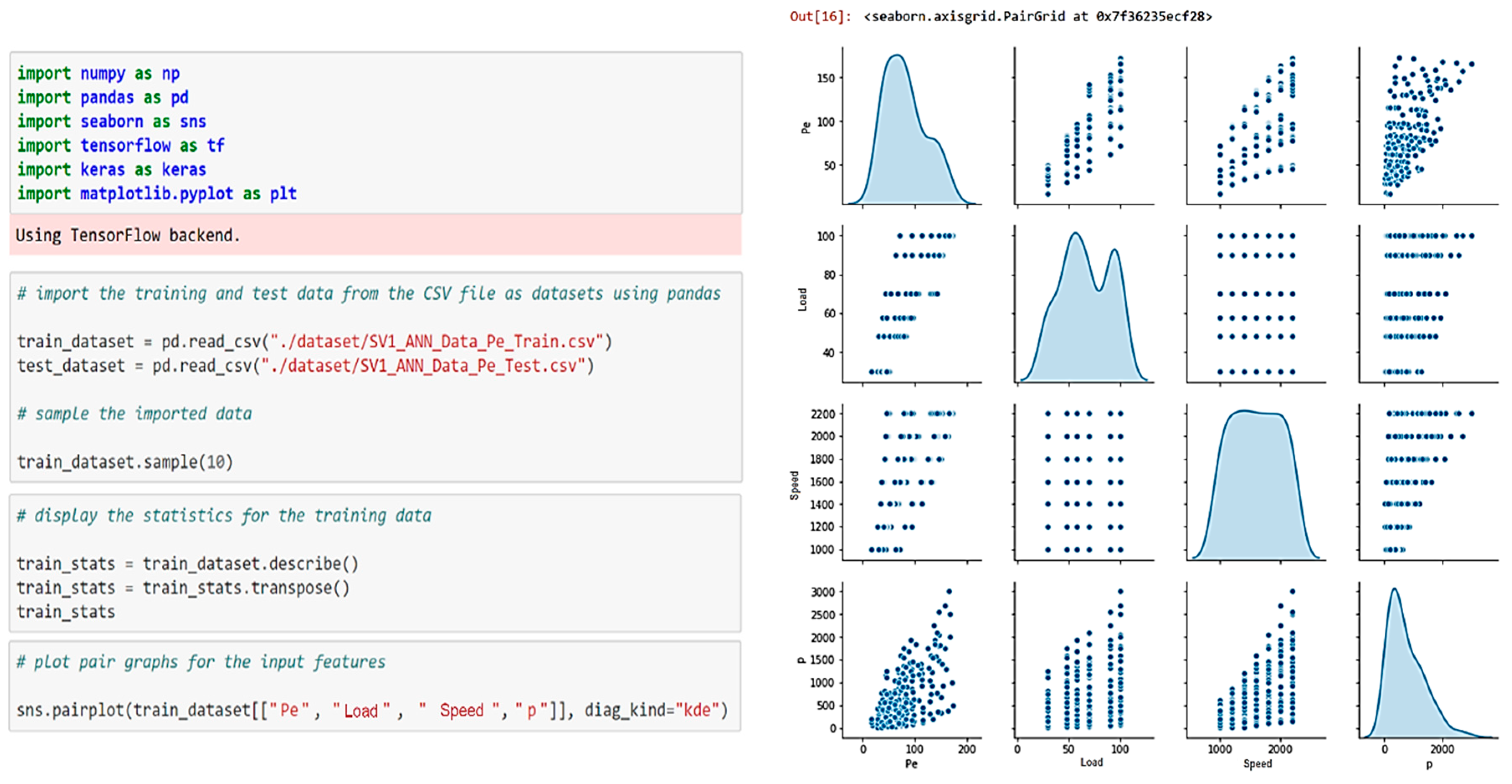
The graphical analysis of the intricated curving shapes in Figure 2 reveals a rather limited number of points that cannot accurately describe the effect of EBP on engine power. Even though the number of 246 experiments is quite high in engine research work, engine control requires a higher granularity of data on an engine performance map. Engine testing procedures are expensive, time-consuming, and need special purpose infrastructure; the number of measured vehicle parameters is limited compared to what can be done with a test-bench, which is why it is highly recommended to complement the experimental data with predictions based on artificial intelligence.

Unlike stand-alone physical sensors, virtual sensors are embedded mini-systems designed to calculate and provide data to ECUs (electronic control units). For the current work, the virtual sensor was basically an ANN or a regressor that was supplied in the normal operation phase with input data from a number of only N physical sensors (e.g., the simplest and/or most reliable and/or cost-effective ones), data used for the estimation of the extra value, indexed (N + 1) that are difficult to measure directly or indirectly via simple calculation formulas. Nevertheless, in the training phase, the AI model was fed with complete datasets, each including (N + 1) values, which were measured on the engine test-bench. In the context of the present investigation, as illustrated in Figure 3, the (3 + 1) variables were engine speed, load, EBP, and power. By applying AI, the fourth variable, effective power, was obtained based on predictions.

For modern ECUs, engine control maps have become very intricate with dedicated hardware/software architectures for each sub-system from air and fuel management to exhaust after-treatment. AI can replace one or more controllers with efficient smart devices that can be integrated into an engine’s ECU; such AI-based solutions are able to facilitate the simultaneous optimization of all apparently contradicting ECU objectives such as fuel economy, lower emissions, and higher torque and power.

In applied sciences, particularly in the field of ICEs (internal combustion engines), AI is frequently used to solve computational-intensive problems such as function approximation, prediction and process control, and the management of the complicated relationships between inputs and output variables. Due to this intrinsic complexity, the following paragraphs aim to restrict the presentation of specific concepts, chosen methods, and developed solutions to smart devices for vehicular applications. Nevertheless, a multi-disciplinary approach is preserved with some conceptual extensions written in quotes.

4.1. Placing AI in a Distributed Computational Environment

The resource-intensive modern methods of computational intelligence [32] often involve cloud computing with theoretically infinite processing power and storage capacity. In Figure 4, these two aspects of computing are distinctively considered.

Centralized versus localized computing extends the cloud computing/edge computing problem to cloud AI/edge AI [33]. Modern telecom technologies of “cyber-critical communications” ensure time constants that are much smaller than those needed for vehicular applications.

Placing AI near the engine, at “the edge” of a test-bench or vehicular appliance, is a multi-criterial decision that considers mainly sensor/transducer signal conditioning, data acquisition, multi-point logging, and pre-processing for compression.

The problem is where the AI-driven “assisted” decision (for real-time automated control) is to be taken. The solutions presented in this paper demonstrate that state-of-the-art technologies enable de-centralized optimal decisions via “edge AI” (Figure 4).

In our vision, smart devices with artificial intelligence should be modelled (in a top–down approach) as FSMs (finite state machines). Appendix B details event-driven models for these smart devices with AI.

4.2. AI Algorithms Applicable to Virtual Sensors

The extensive AI taxonomy [34,35] starts from the challenging paradigm of algorithms that enable computers to solve problems they were not explicitly programmed for.

4.2.1. Artificial Neural Networks

Machine learning (ML) frequently uses ANNs that implement synthetic neurons similar to the cells of the nervous system. The similarity is structural (an ANN is organized into input-/hidden-/output-layers) but mainly functional and based on the ability to learn. As electro-chemical neuro-channels enforce synapses, ANNs can iteratively grow—via different types of successive approximations—some weights to endorse inputs’ specific contributions to intermediary results or outputs. What is making an important difference between ANNs and the computing of simple linear combinations is the “activation” of artificial neuron (weighted sum node) output.

This is very specific to neural signal propagation in the human brain cortex and is fundamental for “triggering” in event-driven models (detailed in Appendix B). To yield the “activated” neuron’s final output y(x), an “activation function” is applied to the preliminary weighted sum x in order to produce the actual output y [36]. For instance, a simple choice that frequently occurs in the next sections of the paper is that of activating the output y = x only for positive x and to inactivate it, y = 0, for the rest. This very simple activation function, ReLU (rectified linear unit) is typical of simple “half-wave rectifiers”. The advantage of being linear is counter-balanced by the disadvantage of being uncompressed.

One of the most useful activation functions is the hyperbolic tangent, y = tanh (x). It compresses the neuron’s output between -1 and 1 and is also quasi-linear in reproducing x around 0 (tanh (x) ≈ x for x ≈ 0, as its derivative tanh’ (0) = 1). There are many activation alternatives; one of them is the “sigmoid”, y = 1/(1 + e^−x), a “scaled” (dividing by 2) and “shifted” (finally adding ⅟₂) version of tanh. For x << 0, the sigmoid is similar to ReLU (that “inactivates”, or nullifies, y for a negative x) and similar to tanh for greater positive x >> 0, with an y also compressed to 1.

The importance of such compression is related to the preliminary “statistical” compression of an ANN’s main inputs (a procedure detailed in the next sections of the paper), which practically becomes a pre-normalization, by first subtracting the mean and then dividing the difference by σ, the standard deviation.

Each normalized sensor output that feeds the ANN is then “statistically 0-centered and compressed” between -1 and 1 (spurious extreme values—possibly caused by sporadic un-systematic errors—are less important). This is very practical for a better use of the ENOB (effective number of bits) at the ADC (analog-to-digital converter) obtained by pre-conditioning the signals (to adapt a sensor’s range to the ADC range), as detailed in Section 6.

The training of an ANN consists of the iterative optimization of the above-mentioned neurons’ weights.

Conventional ANNs use “feed-forward” computations results—from the inputs to the neurons of the first “hidden layer” and so on up to the neurons of the last hidden layer that feed the output(s) neuron(s). In this case, the usual “learning process” uses the “back propagation” (BP) of the updating increments of the weights.

These updates aim to minimize the successive approximation errors between the ANN outputs and the actual (observed and measured) output values of the training set [37]. Iterative optimizations are done according to a chosen criterion, e.g., the minimization of MAE, the mean absolute error, or the minimization of the MSE, the mean squared error. For n-dimensional errors e, MAE and MSE correspond to the L₁ and L₂ norms, respectively, where L_p = $({\displaystyle \sum }_{i=1}^n {\left|e_i\right|}^p ){ }^{1/p}$ [38].

As for the optimization method, iterations aim to reduce (a “descent”) the error (“the gradient”) in a “stochastic” way via successive approximations.

For edge AI solutions, the chosen method was SGD (stochastic gradient descent), which computes a new modification of each ANN weight as a linear combination of the previous modification (its coefficient being the so-called “momentum”) and of the gradient itself (its coefficient being the “learning rate”). In our case, the ANN inputs were load (L), speed (S), and EBP (p), and the output was the effective power (Pe).

4.2.2. Classifier Trees

An important alternative to an ANN is the linear regression tree—each branch (computing a weighted sum with an own set of coefficients) is like an “ANN without activation” decision; this decision is now represented by the switching to another specific branch.

The regression of sub-domains is apparently profitable for training datasets like the ones produced at an engine test-bench with specific load and/or speed “steps”. We explored this alternative of classifier trees using WEKA (Waikato Environment for Knowledge Analysis) [39]. This software environment was used, in the broader context of this paragraph, in several AI algorithm assessments as a comprehensive “workbench for machine learning”.

WEKA encloses many classifiers and regressors (Bayes classifiers, SVMs (support-vector machines) for supervised ML, etc.), as well as decision trees, e.g., ID3 (Iterative Dichotomiser type 3) or C4.5 (improved version of ID3 of the CART—classification and regression tree— type). In other fields of data analytics, e.g., clustering, WEKA offers methods like k-means (for groups of k measurement means) and EM (expectation–maximization) (of the likelihood of a statistical model estimated parameters with the observed data).

The evaluated classifier tree (applied to the engine test-bench dataset), belonging to a fifth category (in reference to the above-mentioned type 3 and 4 algorithms) builds a model (M) via a “divide et impera” procedure, presented in Figure 5. We chose the optimized M5 method (M5P, or the M5 method that has been “pruned” or “trimmed”) that starts with a preliminary data sub-domain division and then applies the linear M5 model to each such sub-domain. The M5P alternatives offered by WEKA included RandomTree (random successive approximation of the tree), RandomForest (random combination of trees), and RepTree (repetitive combination of several trees).

Nevertheless, precaution is needed in adopting tree models: even if training data may exhibit a discrete structure for one or more inputs, this may only be frequent on experimental benches (e.g., in the standard testing of engine duty cycles and/or step-wise dynamometric brake regime) but not in road vehicles use with continuous load and speed variation.

Such a “model contamination” due to a pseudo-discrete input data structure is similar to the “memory effect” caused by scarce training sets; their number can be as low as the number of nodes available in the ANN models—an odd synthesis could even allocate an unwanted individual neuron activated only for the respective single set of inputs and delivering just the particular training output.

5. Cloud AI Implementations

As already mentioned, processing and storage resources in the cloud could be considered “infinite” for our approach, and only communications could theoretically limit the performance of an edge–cloud–edge vehicular smart device implementation. In the following paragraphs, we detail the methods (mainly regressors and ANNs) used for running AI algorithms in the cloud for the common parameters and test-bench datasets introduced in Section 3 and detailed in Appendix A.

5.1. MATLAB in the Cloud

The first centralized AI solution implemented was based on a modern capability to run MathWorks MATLAB™ in the cloud (“MATLAB online”) and a special feature to produce a whole range of AI models that are set to “compete” in the training phase with the option of directly putting the most proficient one into operation. This extends the GAN—generative adversarial (neural) network—principle for the optimal selection of ANN algorithms and/or parameters [40]. The advantage is the cloud MaaS (“Model as a Service”) adaptive offering of the AI algorithm best-suited to a particular optimization problem and/or a particular data structure.

When running this procedure on the training data Pe (L, S, and p), the AI cloud “recommended” the linear Gaussian regressor with the Bayesian optimization (indicated in Figure 6) that uses, for its successive approximations, random variables with a Bayesian distribution that have hyper-parameters (like the learning rate and the error threshold for approximated weight assessment) that are statistically independent and compliant with the Bayes’ theorem of conditional probabilities.

The data uploads in the AI cloud were used to setup MATLAB for the generation of an optimal prediction model for the effective Pe based on the three inputs of load, speed, and p (the EBP—exhaust back pressure); details of the common datasets representation are given in Appendix C.

The regression models offered in the cloud and the optimal choice are presented on the right side of Figure 6.

5.2. Keras API for ANN

The next evaluated implementation alternative was the Keras application programming interface (API), a framework that is a very useful handler of the Tensorflow backend [41].

As supporting libraries, we used NumPy, Pandas, and Seaborn for the creation of “tensors” (the main multidimensional data arrays), data reading, and data analysis, respectively, prior to the model definition.

For the creation and presentation of the various documents required and produced in the Keras implementation, Jupyter Notebook was used. Details of the common training, test data input, normalization, and representation are given in Appendix C.

Figure 7 shows the Keras NN build-up. Each of the two “dense” layers of the ANN had 64 neurons, so, for the three inputs, there were 3 (+1 for the bias) multiplied by 64 = 256 weights for the first layer; for the second layer, there were (64 + 1) × 64 = 4160 weights; and, for the output neuron 64 + 1 = 65 weights, so the total was 256 + 4160 + 65 = 4481 coefficients.

The activation function for the first hidden layer was ReLU, and for the second hidden layer, it was the sigmoid. We tested the optimization (performed via “back-propagation”) using three methods: RMS (root mean square) minimization, SGD (stochastic gradient descent), and SGD’s improved version (in terms of memory usage and running time), the ADAM method [42].

For our Keras case-study (layer 1 (64 neurons), activation function ReLU, and layer 2 (64 neurons), sigmoid activation function), we chose the “optimizer = rms” with the criterion “loss = MSE”, as described in Section 4.1).

The last phase of this Keras flow was the running of the training process depicted in Figure 8. For this purpose, the fit method was invoked for the above-configured model. Five-hundred iteration epochs were ordered (using an own validation_split = 0.2, i.e., 20% out of the normed_train_data).

In order to evaluate this model, the MSE was computed for the testing set. As seen in Figure 9, MSE = 0.01.

5.3. XGBoost API

The eXtended Gradient Boosting (XGBoost) methods [43] are oriented around the iterative optimization of AI classifiers by the “forced” (“boosted”) combination—without their usual invalidation—of some classifiers with apparent lower performances; if considered individually in usual convergence computations, such weaker classifiers could be discharged even from the beginning, being rejected just after the first successive approximations.

A first XGBoost model (xgbooxt-test-raw) was implemented without the pre-normalization of the training and test datasets (the three inputs of load, speed, and EBP and the output of effective power) fed as .CSV (comma separated values) files. A regressor (a combination of linear models) that is quite performant was obtained—as shown in Figure 10, the ratio “explained” variance (of the predicted values)/variance of the observed (test) values gave a score of 0.949760939140567, close to the ideal 1 (with the variance being σ²). The model type was “manually” set by the “booster” parameter for the XGBRegressor (gblinear—as in our case—or gbtree) and, after the training phase, exported (as xgb_model.dat) by the pickle module imported by Python. This model was also used in Section 6.2. As seen in Figure 10, the XGBoost implementation in Python was similar to the Keras handling of Tensorflow models.

The model was run (in the test phase) as described in Figure 11 by “reading the boost” (“rb”) model that was “written” (“wb”) in the training phase.

Exposing the xgb_model.dat as an API can be done with a web micro-server generated with the “Flask” mini-framework programmed in Python. An ‘/api/predict’ HTTP (Hyper-Text Transfer Protocol) “GET” method directly receives its parameters (“load”, “speed”, and “p”) in the URL (Uniform Resource Locator) written in the address bar of the browser, e.g., http://localhost:5000/api/predict?L=90&S=1800&p=250.

The “xgb_model.dat” (imported by pickle into the tiny server.py) returns the “prediction” value.

5.4. Levenberg–Marquardt ANN Implementation via the API of ANNHUB

ANNHUB™ is a machine learning platform offered by ANS Center [44] that is accessible via API calls that we integrated into the National Instruments™ LabVIEW VIs (virtual instruments). If the platform is set to design an ANN for prediction, it automatically chooses the Levenberg–Marquardt (L–M) algorithm. In its particular form for ANN, L–M considers the iterative optimization (in the training phase) of the weights in a compound estimation of the outputs—not only as a function of the inputs but also of the series of state variables. These auxiliary state variables are generally chosen for a formulation of the system’s equations that is as compact as possible. According to control theory, iterative updates of ANN weights can be a “PID” (“proportional–integrative–derivative”) linear combination of the estimation error ε, of its integral ∫ε, and its derivative ε’—e.g., in the L–M multi-dimensional case, “D” (“derivative”) computation is done with the J (Jacobian) matrices of derivation operators (reciprocal partial derivatives of all the variables). In this perspective, the SGD method (briefly described in Section 4), based on gradients, also belongs to the “D” category. Specific to the L–M algorithm is the addition of a “P” (“proportional”) component—the proportionality coefficient is called “damping factor” that is adjusted, in each iteration step, to a smaller value (towards a gradual damping of the “P” part of the updates).

Figure 12 presents the L–M configuration in ANNHUB and the training process with the same 184 + 62 = 246 data sets used in the previous paragraphs; “mu” is the iterative multiplication factor ν that adjusts the damping factor.

In Figure A4 of Appendix C (dedicated to data visualization), one can notice the very good overlay of the predicted outputs on the test outputs and the good value (closed to the ideal 1) of R-squared, which is the “coefficient of determination” (of the actual observed (test) values by the predicted values), i.e., the ratio between the variance of the predicted values (the “explained variance” already mentioned in Section 5.3) and the variance of the unpredicted values.

For various applications of ANNHUB-generated models, at the client-side, different APIs are offered by ANS Center. For a good integration of cloud AI with the instrumentation, the LabVIEW API was chosen. As seen in Figure 13, the cloud AI model can be integrated with a “Create ANN” block only with a “license content” code that can be downloaded (cloud → edge) only after an (edge → cloud) credentials upload.

6. Edge AI Implementations

6.1. Compact ANN Implementation—“AI in a Nutshell”

The objective of this smart device implementation—edge AI for virtual sensing—is a minimal computational foot-print for a “hard-coded” ANN, with coefficients included directly in the firmware, based on a very low cost and compact board (around 10 cm²). This proposed “AI in a nutshell” is built around a popular SoC (system on chip) and is much smaller than usual SBCs (single board computers). The experimental data, introduced in Section 3 and detailed in Appendix A, had 246 sets of N + 1 = 4 test-bench measurements: load (%); rotational speed (rpm); p—EBP (mmWC); Pe (the effective power; in kW). Out of these, 184 sets were randomly chosen for training, and the rest of 62 sets were kept for testing (

Table A2. Partition of the engine experimental data.

The 184 Datasets for Training				The 62 Datasets for Testing
Load	Speed	p	Pe	Load	Speed	p	Pe
100	1000	60	72.1	100	1000	260	72
100	1200	440	94.4	100	1200	270	95
…	…	…	…	…	…	…	…
90	1600	1080	113.7	90	1600	800	114.9
90	1800	600	129.7	90	1800	250	130.3
…	…	…	…	…	…	…	…
70	2000	1380	106.8	70	2000	1560	104.5
…	…	…	…	…	…	…	…
58	2200	1940	92	58	2200	1700	95
…	…	…	…	…	…	…	…
48	1200	570	39.7	48	1200	460	40.6
…	…	…	…	…	…	…	…
30	2200	1260	45.6	30	2200	750	47.9

). The chosen architecture of the compact ANN (with two hidden layers) is presented in Figure 14.

In Appendix A,

Table A3. The normalization reference parameters.

Mean (from the Training Data)		Standard Deviation (from the Training Data)
Load mean [%]	67.08695652173910	std Load [%]	23.45099060386270
Speed mean [rpm]	1602.173913043470	std Speed [rpm]	400.5372101450430
p mean [mmWC]	762.2826086956520	std p [mmWC]	612.5875771655360
Pe mean [kW]	82.76250000000000	std Pe [kW]	38.92861019322530

presents the normalization reference parameters. It is assumed that the statistics were meaningfully contained in the comprehensive training data. The mean and the standard deviation (σ) values were used extensively, not only for the preliminary normalization but also for the final de-normalization in the virtual sensor. Any future “statistic re-calibration” of the edge AI smart device should update not only the ANN weights but also these de-/normalization reference parameters.

The programming system chosen for development of the compact ANN is given in

Table 2. The software environment for the development of the “edge AI” ANN (see also Section 5.2 and Section 5.3).

Name	Description	Scope
PyCharm	Integrated development environment (IDE)	Software development in the Python programming language
NumPy	Libraries package for the Python programming of scientific computation	ANN training	ANN use
PyTorch	Python version of the Torch libraries with methods dedicated to artificial intelligence	ANN training
Pandas	Python libraries dedicated to matrix computation	ANN training

.

The “AI in a nutshell” demonstrator was implemented with a cost-effective micro-module, TTGO™, recently marketed by LILYGO, built around a “WROOM-32” module produced by Espressif [45] and the well-known ESP32 SoC. Edge-computing local resources are: 4 MB flash program memory, 8 MB PSRAM (pseudo-static RAM) of working memory, and a CP2104 UART (universal asynchronous receiver-transmitter) chip.

The outstanding ESP32 capabilities are the WiFi (802.11 b/g/n) and Bluetooth 4.2 BLE (low energy) protocol with BR/EDR—basic rate/enhanced data rate.

A convenient organic LED (OLED) display (128 × 64 pixels) is managed by an SSD1306 I2C (inter-integrated circuit) interface chip. As seen in Figure 15, the micro-module also has a T-camera, a PIR (passive infra-red) AS312 sensor and a BME280 barometric environmental sensor.

Such a versatile LILYGO micro-module does not have many extra GP-I/O (general purpose input/output) pins left, so three direct wired connections were added to the two multiplexed inputs of ADC2 (GPIO 2 and 26 to channels 2 and 9) and, respectively, to channel 6 of ADC1 (GPIO34)—for this last connection, the 10 kΩ pull-up to 3.3 V was interrupted.

In order to comply with the 3.3 V supply voltage requirements of this CMOS (complementary metal-oxide-semiconductor) board and many others, the three ADC inputs had to be brought, in advance, in the 0–3.3 V interval. This means they could not be taken directly from the outputs of different kinds of sensors and needed an intermediate signal conditioning, detailed in Section 7.2 and Appendix E.

For the above-mentioned chosen ANN architecture, in both hidden layers, the chosen activation function was ReLU (without compression but linear and, most notably, the simplest to implement in a compact code).

As introduced in Section 4.2.1, the chosen BP optimization method was SGD, with the NN (neural network) benchmark “nn.L1Loss” (minimizing MAE, according to the L1 norm, is one of the most robust criteria).

The value of the momentum was 0.9, and the learning rate was lr = 0.001.

After 5000 “epochs” (the number of BP optimization iterations) running on the normalized training data (182 sets), 10 × 3 = 30 coefficients “hidden1_weight” coefficients and 10 × 1 = 10 “hidden1_bias” terms (for each neuron’s linear combination of 3 inputs, a free term is added) were obtained for the three inputs in the 10 neurons of the first hidden layer. For the second hidden layer, 10 × 10 = 100 coefficients “hidden2_weight” coefficients and 10 × 1 = 10 “hidden2_bias” terms were computed.

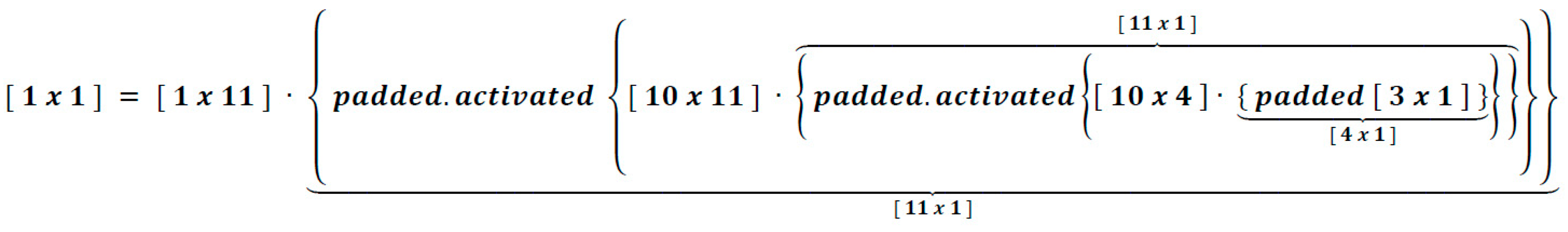
In the ANN run, the main ANN “exploitation phase” (and also for the testing detailed in the following), the coefficients obtained after the training phase could be grouped in tables for a compact matrix calculation. The [1 × 1] result was not obtained via the simple multiplication (starting with the column vector [3 × 1] of the three inputs written to the right in the following product) [1 × 1] = [1 × 10] ∙ [10 × 10] ∙ [10 × 3] ∙ [3 × 1]. Instead, as seen in Figure 16, there are needed three preliminary paddings with 1 elements at the right-side factors: for the [3 × 1] input and for the two [10 × 1] activated hidden layers’ outputs. Accordingly, it was needed three times, a correspondent padding of the weights arrays with the column vectors of the biases - at the left-side matrix factors:

As depicted in Figure 17, a 10 × 4 “layer1Weights” array was obtained from the 10 × 3 = 30 coefficients “hidden1_weight” array padded with the 10 × 1 = 10 “hidden1_bias” column vector, and a 10 × 11 “layer2Weights” coefficients array was obtained from the 10 × 10 = 100 “hidden2_weight” coefficients array padded with the 10 × 1 = 10 “hidden2_bias” column vector.

More than half of this very compact code was represented by the embedded coefficients—an efficient solution that does not require reading of .CSV or similar formatted tables from an “external file system” that would misuse the reduced resources of such a tiny board.

6.2. NVIDIA Mini-System with Hardware Acceleration of AI Computing

A “cutting-edge” solution—aiming to demonstrate one of the most powerful AI resource concentrations at “the edge” of the network—was based on the NVIDIA Jetson Nano (V3); see Figure 18. Though this development kit is remarkable compared with the features of a usual SBC (single board computer), it is quite cost-effective (priced less than twice that of an average SBC).

The mini-system is driven by a four-core advanced RISC (reduced instruction set computing) machine “ARM” A57 processor with 4 GB RAM 64 bit LPDDR4 (low-power double data rate) with 25.6 GB/s), multiple high efficiency H.264/H.265 video codecs, Ethernet 10/100/1000BASE-T, and many other general-purpose interfaces. The dedicated AI software was installed on top of the Linux OS with TensorRT libraries for “deep learning”.

The main sub-system was the 70 × 45 mm Jetson Nano SOM (“system on module”), with a special parallel NVIDIA “Maxwell” processing unit. This hardware, directly allocated to ultra-fast AI computations, has a structure inspired by parallel architectures of the graphic processors with GPC (graphics processor cluster) chips—each cluster having 5 SMs (streaming multiprocessors). Parallelism is essential for the “systolic” ANN computations, given the neurons placement and the “wave” transmission of data flows for the forward propagation (FP).

The Maxwell architecture sustains the “neuromorphic computation”:

−

The SMs have processing units with Kernel preemption (a compromise between the prioritization and parallelism of the processes). These units are called “CUDA (compute unified device architecture) cores”, with each core having two computing sub-systems (for integers and for real numbers with floating point) and 16 load/store blocks.

−

A Maxwell chip has 128 CUDA cores interconnected by a fast NVLink bus which has a high bandwidth memory (HBM2 - up to 59.7 GB/s).

−

Each SM has 64 K (=65,536) registers of 32 bits and can run up to 64 warps (a “warp” is a grouping of 32 threads for the parallel execution of an instruction).

In all the software part of the NVIDIA-based implementation, described as follows, some capabilities that were considered, until now, as cloud-specific could be observed. For instance, this edge-computing solution used its own embedded server exactly as described in Section 5.3. Most remarkably, it transfers data using local web services for methods invoking API and for “publishing” results. This complies with REST (REpresentational State Transfer) [46], the modern approach of the state-driven models (mentioned in Appendix B). The “RESTful” transition in/out signaling is done via HTTP and parameters in/out are embedded in GET (or POST) messages’ attributes directly in the URLs.

On the NVIDIA Jetson Nano, an LXDE—light-weight X11 (version 11 of the X Windows display protocol)—DE (desktop environment) was installed for intranet(/internet) access compatible with the X2Go server. In this environment, with “pip3 install” commands, the following were configured: xboost, pandas, sklearn (like in Section 5.3), and the flask server (that enables ANN computations to be invoked via APIs like in the cloud solution described in Section 5.3 but now locally). Prior to xboost installation, with the “cmake” command, compilation was done with the explicit activation of the CUDA-based hardware acceleration: cmake. -DUSE_CUDA=ON. In Figure 19, it can be seen how the flask server is started (listening on port 5000 and exposing its services to the localhost) and how the HTTP command GET is invoked via the above-mentioned xboost API: the AI method “predict”. This method computes Pe for ANN inputs given as attributes of the GET message—L = 100 (%), S = 1000 (rpm), and p = 80 (mmWC)—included in the URL written in the address bar of the browser.

Using a DDNS (dynamic domain name server) a simple port forwarding may be configured on a local router to extend intranet-to-internet access using a public IP address. This modern approach became “distance-agnostic” (with the same transfers locally or remotely)—a real ubiquitous and mobile computing solution that could be installed either on the engine test-bench or on vehicles.

7. Results Interpretation

7.1. ANN Test Flow via Dedicated Virtual Instrumentation

For a thorough verification of all the ANN calculations with a totally separated test flow, a dedicated National Instruments Virtual Instrument was built in LabVIEW. The virtual instrument (VI) diagram (detailed in Appendix D) illustrates how test data, individually or as a block (of 62 sets in our main use case, exercised in most other implementations, Section 5.1, Section 5.2, Section 5.3, Section 5.4 and Section 6.1), could be fed as an Input.csv file, together with the reference parameters computed from the statistic of the training data (184 sets in our main use case): the Means.csv and StdDev.csv files, as detailed in Appendix A.

The implemented virtual instrument could be used for various ANN coefficient sets (weights and bias parameters) for more two-layer models with ReLU activation. Specifically, the versatility of this VI implementation is given by its scalability to changes in the dimensions of the two hidden layers that can have even different numbers of neurons/layers.

Figure 20 shows four examples of the compact code (6.1) run with the corresponding virtual instrument (VI) test verifications.

For this “edge AI” smart device presented in Section 6.1 (“AI in a nutshell), the ANN verification is given in

Table 3. “Embedded” ANN performance assessment for the 62 normalized test values of Pe.

Pe Normalized	Pe Normalized Estimated	Squared Error
−0.276467615	−0.265836447	0.000113022
0.314357485	0.329886377	0.000241146
…	…	…
−0.895549567	−0.890819013	0.000022378

MSE = 0.000593327; the square root of MSE results RMSE = 0.024358305. The relative precision of the estimation, $\frac{\mathrm{RMSE}}{2}$ (after dividing by the interval [σ − (−σ)] normalized, i.e., [1 − (−1)] = 2) = 1.218%.

.

As the optimization criterion was MAE, the mean of the absolute error, 0.01992755, was also considered relevant. Half of this value gives a relative precision of the estimation equal to 0.9963%. The interpretation of precision as relative to standard deviation is a matter of discussion; in this case, RMSE division should have been done not to 2σ but to larger intervals up to max–min. For such cases, the relative precision would be significantly better. However, spurious extreme values, erroneous measured values that happen to be outside the inputs’ statistic (even if occurring once), can make the max–min difference a “span” that is useless as reference for the precision. Regarding such “outliers”, the MAE criterion is more robust (due to the squaring of the errors, the MSE was more distorted by spurious inputs).

As seen in Figure 17, the 12 bit outputs of the ADC, between 0 and 4095 = 2¹² − 1 (for the converters’ analog input range 0–3.3 V as detailed in Appendix E), were re-shifted by subtracting 2048 (half of the binary span). Re-scaling was not done by division to 2048 but to 4096 (written 4096.0, to switch the computing into real numbers). This means that, related to normalization, inputs should be allowed to be between −2σ and 2σ and not only between ± σ. This compromise (the overlaying of the less probable greater inputs) only affected the MSB (most significant bit) of the digital input.

Nevertheless, the greater time-constants in vehicular applications (particularly in diesel engine ECUs) allow for some over-sampling of inputs (even if analog channels are multiplexed to the input of a single ADC)—e.g., with a sampling frequency 2ⁿ times greater than f_Nyquist (double the maximum frequency in the spectrum of the continuous signal), an effective number of bits, ENOB = n + the number of bits/sample at the ADC output, can be obtained if a moving average (with a 2ⁿ broad window centered on each ADC output) can be computed.

7.2. Signal Conditioning

Before being submitted to the analog-to-digital converters of the tested smart devices, the different kinds of signals offered by the various types of sensors have to be pre-conditioned. Most of this signal conditioning is a “scale and shift” pre-processing; for instance, for the 6.1 edge AI solution, the sensors output signals had to be brought in the above-mentioned 0–3.3 V interval. The external add-on miniature sub-systems for signal conditioning are presented in Appendix E.

To close a calibration loop for each physical sensor path, the extra multiplicative factors should be adjusted iteratively (starting with 1) not in this signal conditioning module but, more conveniently, directly in the software, increasing or decreasing the shift step (e.g., 2048; see Figure 17) and/or the re-scaling denominator (e.g., 4096; see Figure 17). For instance, to calibrate the “load” channel, the two corresponding iterations had to equal the displayed load with 100 (on the mini OLED screen) if the actual load was exactly 100% on the engine test-bench.

7.3. Comparison of the AI Solutions for Smart Devices

For all the six main implementations, the same train and test data (with 184 and 62 measurement sets) was used. This was an important common base for the comparison presented in Figure 21.

For the needs of comparison, some of the longer decimals groups could have been truncated (to only n, where 10⁻ⁿ ≤ sensors accuracy). Nevertheless, for an easier reference, the benchmark scores were left with the digits after the decimal point exactly as displayed by the various calculation results in Section 5 and Section 6. As shown in the performance column, some of the precision figures had to be normalized (either dividing by mean Pe = 82.76 kW or by σ − (−σ) = 2σ (=2, normalized)). As the compact solution of Section 6.1 “edge AI” is both ANN-based and hardware- and software-implemented, it was necessary to use it as reference, so both precision benchmarks (relative to RMSE and to MAE) were calculated for this “AI in a nutshell” smart device.

Due to the large number of neurons in its two “dense” hidden layers (a total of 129 neurons with a total of 4481 coefficients), the Keras ANN (Section 5.2) had a better precision (relative to RMSE).

There are two solutions based on XGB (Section 5.3 and Section 6.2), as well as the solution of Section 5.4 based on an ANN trained with the L–M algorithm, that can be assessed by the R² benchmark, R Squared—the ratio between the variance of the predicted values (the “explained variance” already mentioned in Section 5.3) and the variance of the unpredicted values (it was not considered the R-Squared = 1 label in Figure 6, for the optimized GPR (Gaussian process regressor) solution of Section 5.1).

A comparison between the solutions of Section 5.4 versus those of Section 5.3 and Section 6.2 could be done because the statistics of the training and the measured (observed) actual values were adopted as well for the predicted values (to allow for the quick de-normalization for any individual input).

Thus, in this particular case, the variance of the actual values = variance of the predicted values + variance of the prediction errors, i.e., total variance = explained variance + unexplained variance. The predicted values were totally un-correlated with the prediction errors (this is why they could not explain the statistics of the values and of their predictions). Thus, in this particular comparison, the explained variance score ≡ R² (a common benchmark for the comparison of the solution of Section 5.4 with those of Section 5.3 and Section 6.2).

8. Discussion

The experimental investigations performed on the engine test-bench confirmed the influence of EBP on engine performance that had been previously reported in literature. Within the limits of the EBP variation of the present study, which was 3000 mmWC (=29.43 kPa) at the rated speed and load, the maximum engine power loss reached 3.62%, the BSFC increased with 7.32%, the exhaust gas temperature rose with 100 °C, and the boost pressure decreased with 30% (Appendix A).

The implementation of AI into vehicular sensor data processing regarding the computational allocation (local and/or centralized) in the distributed environment was discussed.

The cloud-/edge-computing (processing–storage–tele-transmission) was extended in a cloud AI/edge AI paradigm that was used for the next sections.

The state-control approach of smart devices (detailed in Appendix B) can be expanded to the ECUs (electronic control units) that also have on-board real-time diagnosis features and optimal decision capabilities.

All the needed parametrization can be adaptive (mostly via ANN), and all the needed transitions can be decided upon with classifiers and other AI means. Such a finite state machine model can also distribute the localized/centralized tasks according to the edge AI/cloud AI extension of the edge-/cloud-computing paradigm.

The second part of Section 4 presented the AI algorithms applicable to virtual sensors, emphasizing ANN and then classifiers and regressors. The resource-intensive parts of AI computation were considered, at first, in the cloud with “infinite” processing power and/or storage capacity (Section 5)—the machine learning parts starting with training of the models and up to the adversarial comprehensive model choice “MaaS” (Model as a Service) introduced in Section 5.1 dedicated to MATLAB in the cloud.

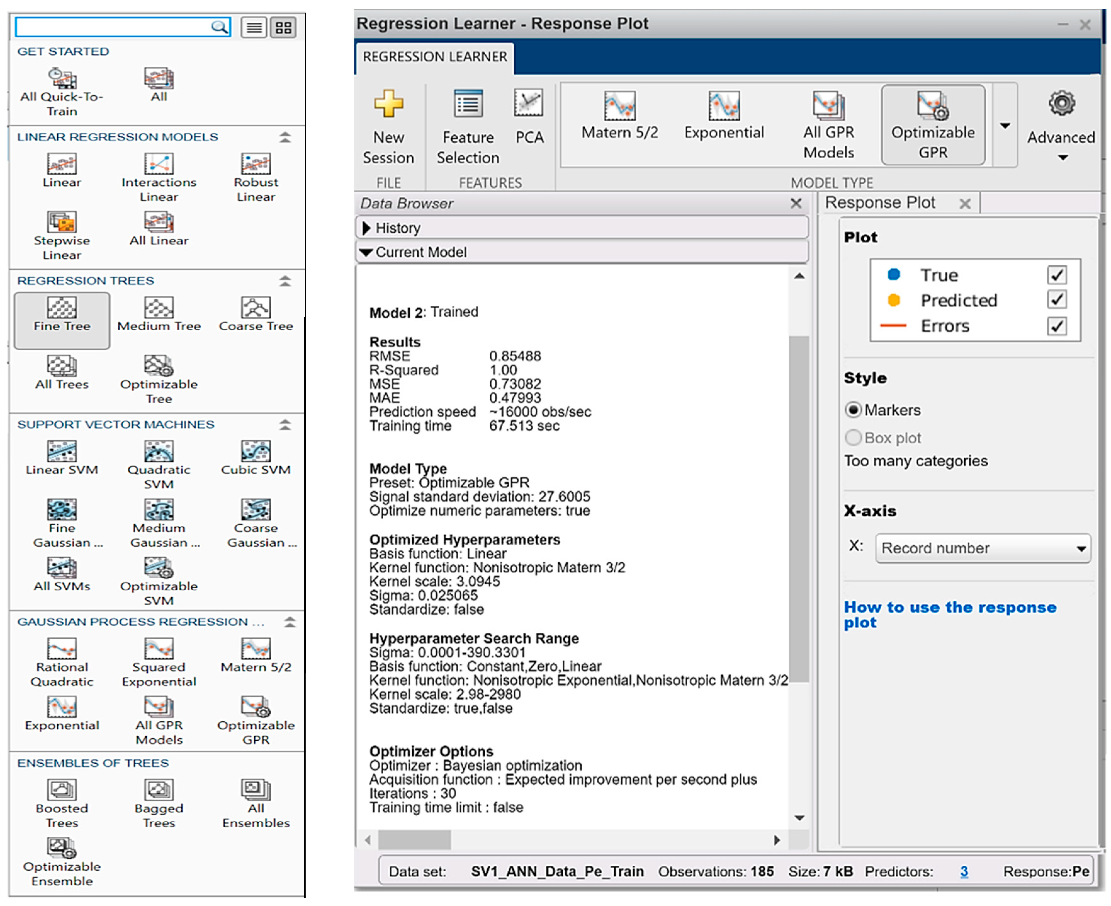
On the unique training and testing data set used in all the use-cases, MATLAB has chosen optimized GPR (Gaussian process regressor) as the best MaaS invoked via API (application programming interface).

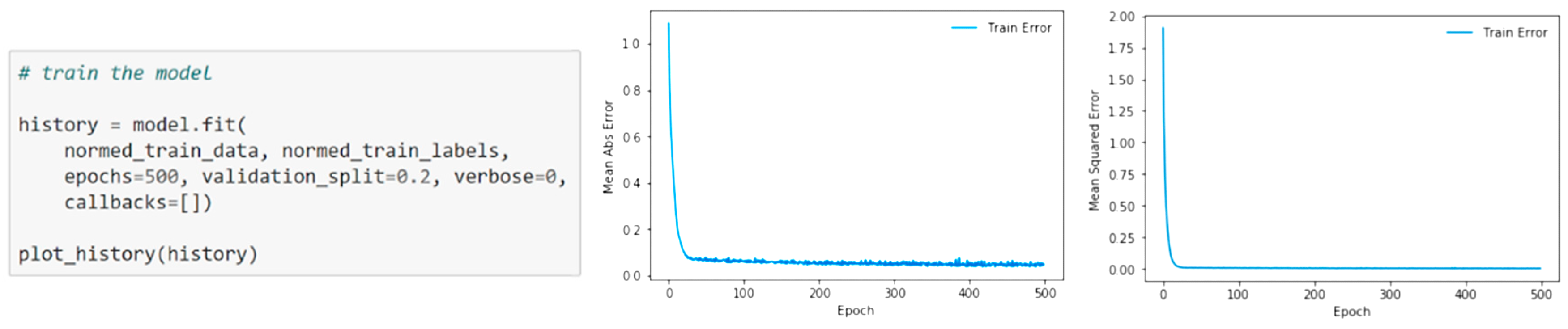
The next cloud AI solution was a Keras API for ANN. The backend computing was based on Tensorflow libraries handling the main multidimensional data arrays as “tensors”. It was obtained a competitive “dense” ANN, with many neurons per layer—a step towards WNN (“wide neural networks”) up to the modern DNNs (“deep neural networks”) with many layers.

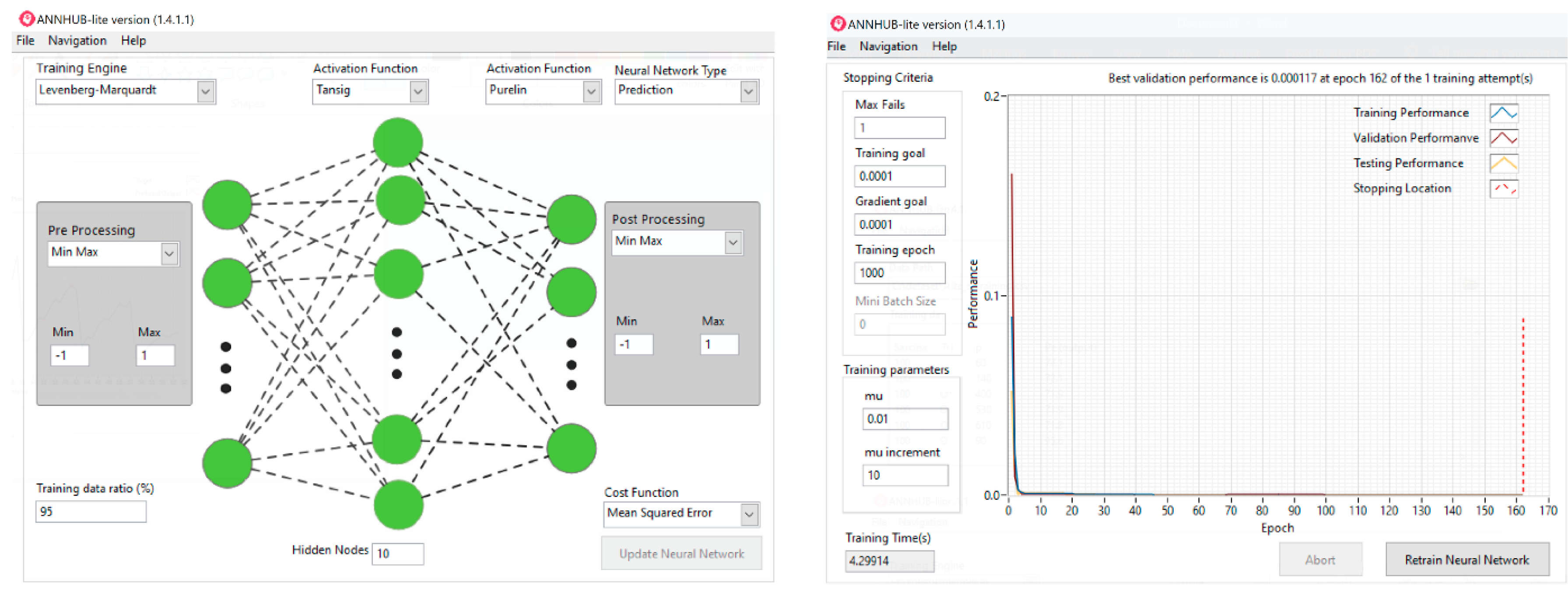
The other two API-accessed cloud AI solutions were based on “XGBoost” (XGB eXtended Gradient Boosting—of iterative optimization classifiers) and on the ANNHUB access to an effective Levenberg–Marquardt ANN.

The cloud AI approach always has the advantage of MaaS computational-intensive features. Besides the example of Section 5.1, the solution of Section 5.3 has also an impressive “automatic” option, GridSearch (offered by the dedicated Sklearn library) for the optimal choice out of a bunch of models trained with more combinations of parameters.

The MaaS features can be considered a future-proof capability in the trend of “continuous optimization” (powered by AI) of the running algorithms that could extend the nowadays “continuous deployment” of micro-services in the cloud.

Accessing AI cloud computations can be used also in mixed solutions, starting with edge DAQ (data acquisition) and data logging in the cloud and up to “AI caching” in the cloud (of the edge computations)—a measure that is useful for intermittent connectivity that is frequently seen in vehicular use-cases.

Even the most compact micro-boards described in Section 6 could easily transfer the N locally-acquired sensor outputs to the cloud that should return the N + 1 (virtual sensor) output in real-time as result of a prediction calculation.

The two solutions proposed based on the same virtual sensor use-case are state-of-the art (referring to the actual market).

The edge AI mini-system with hardware acceleration can take over whole AI types of computing tasks; part of these computing tasks are usually present in the cloud as the model training phase (even for the above-mentioned DNN).

The NVIDIA Jetson Nano small-form factor mini-system, managed by an ARM A57 four-core processor (running a full range of AI software and a Flask micro-server on top a Linux OS) is built around a NVIDIA Maxwell SOM (system on module). In Section 6.2, it was demonstrated how this solution can locally perform the complete range of XGBoost computations that were first introduced as an accessible cloud AI solution (Section 5.3). Most of the cloud AI solutions presented in Section 5 were trained offline. The SOM implementation (Section 6.2) is the only one powerful and versatile enough for real-time edge–cloud–edge future solutions, with the training data upload/(re-)training of the model (and adversarial choice or optimization in the cloud)/download and running of the most advanced (updated or new, not only ANN) versatile model that might also have in-depth scalability. Nowadays, as smartphones have CPU/GPU/APU (central/graphical/AI processing units), this paper is endorsing an edge AI vision on engine instrumenting and control. A Jetson Nano stand-alone “palm” mini-system, even if operating locally, preserves a cloud-like server control that is “distance agnostic”. This means it is feasible a scenario of training data to be fetched from the complete instrumentalized testbed directly to such a small Jetson Nano possible “AI add-on” to the ECU, with a new model (re-)training, even for the limited update needs of “statistical re-calibration”.

At the other extreme, the very compact edge AI solution “in a nutshell” built around a super-miniature board of the TTGO™ series manufactured by LILYGO is centimeter-sized and includes also an OLED mini-display for the three inputs (load, speed and pressure) and the output (Pe). At this super-miniature extreme, though the micro-board includes a tiny digital camera, too much image processing is impossible. Currently, there are promising efforts to optimize AI software libraries—e.g., the new Arduino TinyML (“machine learning”) suite that allows for the compilation of ML models with a new TensorFlow™ Lite sub-set and code upload on micro-modules managed by the Arduino IDE (“integrated development environment”).

The compact edge AI implementation of the smart device directly includes the ANN coefficients (weights and bias) in the code. These coefficients might be simply embedded in the firmware of the virtual sensors. As shown in Section 7.2, any calibration problem becomes a software update problem. Assuming that inputs’ statistics (mean and std dev) do not change in the long-term (without any retrofits in the exhaust and other auxiliary systems of the engine), such a “statistical re-calibration” of the smart devices is seldom needed; in this cases it is sufficient a simple ANN retraining using the fully instrumentalized test-bench. For instance, for the “AI in a nutshell” compact solution of Section 6.1, the new coefficients (the two arrays illustrated in Figure 17) that should be re-loaded in the Flash memory of the micro-board are updated in the code.

An intermediate edge AI solution (a compromise between implementations like those of Section 6.1 and Section 6.2) could involve a “bare-metal” SBC (single board computer—e.g., the very popular Raspberry Pi) that runs a dedicated Docker container. Such a container (the ideal compromise of the virtual machine principle and of the stand-alone compiled executable code) could integrate the environment strictly required for the execution of the AI model without the need to separately install, for instance, Python and the Tensorflow libraries specific to AI.

Cloud AI solutions do not usually provide access to a trained model. This should not be a problem due to API access—a convenient alternative used even for the advanced edge AI solution of Section 6.2 (that, as already mentioned, shares the XGBoost computations with the Section 5.3 cloud AI solution).

Even if known and “finite” at the end, a cloud-trained model might need intensive computing in order to be chosen and calculated. However, as shown in Section 4.2.2 (where a tree classifier was developed with the M5P algorithm of WEKA), precaution is needed when adopting regression models (Section 5.1, Section 5.3, and Section 6.2) that are susceptible to contamination by a pseudo-discrete structure of the training data. From this point of view, the ANN solutions (Section 5.2, Section 5.4, and Section 6.1) could be preferable.

ANNs have other advantages—mostly if the coefficients are individually known and handled for different needs of the implementation (e.g., embedded at the quasi-firmware level in the solution of Section 6.1). ANNs are prone to extrapolations (e.g., to predict the output for inputs that are beyond the range of those use in the training phase). In a classifier tree (mostly with an unknown model—e.g., cloud AI), there is still the risk such inputs not having a branch into which to be routed—such inputs might be considered “outliers”, and the computing system may decide to drop them out. For instance, if EBP is distanced with more times σ from the mean, an ANN may still give an estimate of Pe and predictable behavior for an extended input range, that represents a significant practical value for the AI-based virtual sensor. For example, considering the edge AI solution of Section 6.1, the re-scaling of the 12 bit outputs of the ADC should be done using a scaling numerator greater than 2048 or even than 4096. The pre-conditioning of the signal (according to Section 7.2) should be done accordingly with a greater input divider factor that compresses more of the EBP sensor’s output.

Regarding the computational overhead trade-off with the cost of the solutions, increasing the ENOB (effective number of bits), increasing the sampling frequency or even the number of artificial neurons should be limited by some merit factors like 1/(sensors accuracy) at the test-bench. Such limitations mean that solution assessment should consider not only the algorithms performance (the computational efficiency) or the accuracy of the estimations but also practical aspects like the positioning (edge-/cloud-AI) and all the telecommunication issues and the deployment (up to the above mentioned “continuous optimization” according to the modifications of data characteristics).

9. Conclusions

This paper is centered on the influence of EBP on diesel engine performance parameters. Experimental results on instrumentalized engine test-beds were supplied as training data to ANNs and regressors. These could be further used in stand-alone reliable smart devices for the accurate prediction of power loss versus externally applied EBP in a whole load/speed engine operation. Two practical virtual sensors were implemented as cost-efficient edge-AI solutions. One has an extreme local computational performance (AI with hardware acceleration). The other one has an extreme compactness (hardware miniaturization and minimal code).

The main benefits of the research work are emphasized below.

The experimental investigation has enriched the relatively scarce literature on engine EBP-power dependency.

The continuous development software paradigm was extended to the continuous optimization concept beyond the ANN versus regressors traditional trade off. Though the pseudo-discrete nature of decision trees and outliers’ treatment favored the ANNs, it was shown that the automatic selection or update of AI models is now possible in the cloud.

The implementations were framed by an extended range of criteria and a broader perspective that includes benchmarks, scalability, activation, signal conditioning, and computational resource allocation for new requirements like extrapolation and calibration.

Striving for constructive details, the state-of-the-art practical solutions aimed to rise the TRL (technology readiness level).

The novelty brought by the present work is as follows.

To the knowledge of the authors, the application of AI in engine power loss caused by EBP has not been previously reported.

The cloud AI–edge AI approach supported the applied research of artificial intelligence allocation in the distributed environment.

The MaaS adversarial choice of the AI model in the cloud was demonstrated with two APIs (MATLAB and XGB).

The design flow was extended in a distance agnostic AI chain using Jetson Nano. This complete demonstrator with hardware acceleration could be an ECU add-on capable of the real-time updating of model parameters and even of model type; the flask server solution and seamless XGB regressor download illustrates a “model-agnostic” capability.

The compactness of the hardware in the embedded micro-system demonstrator was complemented by a code-optimization with ANN coefficients in the firmware and put an “embedded AI” solution into practice. It was shown that these coefficients are suitable with the sporadically offline statistical recalibration of the “AI in a nutshell” smart device.

During the applied research on vehicular smart devices driven by artificial intelligence, a real effervescence of innovative solutions was very obvious—the “AI cloud inside” printed on some commercial modules is still a wish today, but it is almost certain tomorrow.

References

1. Wallace, F. Compound and other engine systems. In Diesel Engine Reference Book, 2nd ed.; Challen, B., Baranescu, R., Eds.; Butterworth-Heinemann: Oxford, UK; Waltham, MA, USA, 1999; pp. 75–87. [Google Scholar]
2. Dieselnet. Available online: https://dieselnet.com/ (accessed on 15 August 2019).
3. Hield, P. The Effect of Back Pressure on the Operation of a Diesel Engine. Maritime Platform Division, Defense Science and Technology Organization, Australian Government: DSTO-TR-2531. 2011. Available online: https://apps.dtic.mil/sti/pdfs/ADA542327.pdf (accessed on 26 August 2019).
4. Guan, B.; Zhan, R.; Lin, H.; Huang, Z. Review of the state-of-art of exhaust particulate filter technology in internal combustion engines. J. Environ. Manag. 2015, 154, 225–258. [Google Scholar] [CrossRef] [PubMed]
5. Sapra, H.; Godjevac, M.; Visser, K.; Stapersma, D.; Dijkstra, C. Experimental and simulation based investigations of marine diesel engine performance against static back pressure. Appl. Energy 2017, 204, 78–92. [Google Scholar] [CrossRef]
6. Cong, S.; Garner, C.P.; Mctaggart-Cowan, G.P. The effects of exhaust back pressure on conventional and low- temperature diesel combustion. Proc. Ins. Mech. Eng. Part D J. Automob. Eng. 2011, 225, 222–235. [Google Scholar] [CrossRef]
7. Roy, M.M.; Joardder, M.U.H.; Uddin, M.S. Effect of engine backpressure on the performance and emissions of a CI engine. In Proceedings of the 7th Jordanian International Mechanical Engineering Conference, Amman, Jordan, 27–29 September 2010. [Google Scholar]
8. Mittal, M.; Donahue, R.; Winnie, P. Evaluating the influence of exhaust back pressure on performance and exhaust emissions characteristics of a multi-cylinder, turbocharged and aftercooled diesel engine. J. Energy Resour. Technol. 2015, 137, 032207. [Google Scholar] [CrossRef]
9. Burnete, N.; Moldovanu, D.; Baldean, D.L.; Kocsis, L. Studies Regarding the Influence of Exhaust Backpressure on the Performances of a Compression Ignited Engine. In Proceedings of the European Automotive Congress EAEC-ESFA 2015, Bucharest, Romania, 25–27 November 2015; Andreescu, C., Clenci, A., Eds.; Springer: Cham, Switzerland, 2016; pp. 141–149. [Google Scholar] [CrossRef]
10. Olin, P. A Mean-Value Model for Estimation of Exhaust Manifold Pressure in Production Engine Applications; SAE Technical Paper 2008-01-1004; SAE: Warrendale, PA, USA, 2008. [Google Scholar] [CrossRef]
11. Castillo, F.; Witrant, E.; Dugard, L.; Talon, V. Exhaust Manifold Pressure Estimation Diesel Equipped With a VGT Turbocharger; SAE Technical Paper 2013-01-1752; SAE: Warrendale, PA, USA, 2013. [Google Scholar] [CrossRef] [Green Version]
12. Wang, Y.Y.; Haskara, I. Exhaust pressure estimation and its application to variable geometry turbine and wastegate diagnostics. In Proceedings of the 2010 American Control Conference, Marriott-Waterfront, Baltimore, MD, USA, 30 June–2 July 2010; pp. 658–663. [Google Scholar]
13. He, Y.; Rutland, C.J. Application of Artificial Neural Networks in engine modelling. Int. J. Eng. Res. 2004, 5, 281–296. [Google Scholar] [CrossRef]
14. Jain, A.K.; Mao, J.; Mohiuddin, K.M. Artificial Neural Networks: A tutorial. Comput. J. 1996, 29, 31–44. [Google Scholar] [CrossRef] [Green Version]
15. Cay, Y.; Cicek, A.; Kara, F.; Sagiroglu, S. Prediction of engine performance for an alternative fuel using artificial neural network. Appl. Therm. Eng. 2012, 37, 217–225. [Google Scholar] [CrossRef]
16. Bietresato, M.; Calcante, A.; Mazzetto, F. A neural network approach for indirectly estimating farm tractors engine performances. Fuel 2015, 143, 144–154. [Google Scholar] [CrossRef]
17. Sekmen, Y.; Gölcü, M.; Erduranli, P.; Pancar, Y. Prediction of performance and smoke emission using Artificial Neural Network in a diesel engine. Math. Comput. Appl. 2006, 11, 205–214. [Google Scholar] [CrossRef] [Green Version]
18. Celik, V.; Arcaklioglu, E. Performance maps of a diesel engine. Appl. Energy 2005, 81, 247–259. [Google Scholar] [CrossRef]
19. Parlak, A.; Islamoglu, Y.; Yasar, H.; Egrisogut, A. Application of artificial neural network to predict specific fuel consumption and exhaust temperature for a diesel engine. Appl. Therm. Eng. 2006, 26, 824–828. [Google Scholar] [CrossRef]
20. Rahimi-Ajdadi, F.; Abbaspour-Gilandeh, Y. Artificial neural network and stepwise multiple range regression methods for prediction of tractor fuel consumption. Measurement 2011, 44, 2104–2111. [Google Scholar] [CrossRef]
21. Canakci, M.; Ozsezen, A.N.; Arcaklioglu, E.; Erdil, A. Prediction of performance and exhaust emissions of a diesel engine fueled with biodiesel produced from waste frying palm oil. Expert Syst. Appl. 2009, 36, 9268–9280. [Google Scholar] [CrossRef]
22. Kumar, S.; Srinivasa Pai, P.; Shrinivasa Rao, B.R. Artificial Neural Network based prediction of performance and emission characteristics of a variable compression ratio CI engine using WCO as a biodiesel at different injection timings. Appl. Energy 2011, 88, 2344–2354. [Google Scholar] [CrossRef]
23. Rida, A.; Nahim, H.M.; Younes, R.; Shraim, H.; Ouladsine, M. Modeling and simulation of the thermodynamic cycle of the diesel engine using neural networks. IFAC PapersOnLine 2016, 49, 221–226. [Google Scholar] [CrossRef]
24. Ganapathy, T.; Gakkhar, R.P.; Murugesan, K. Artificial neural network modeling of jatropha oil fueled diesel engine for emission predictions. Therm. Sci. 2009, 13, 91–102. [Google Scholar] [CrossRef]
25. Obodeh, O. Evaluation of artificial neural network performance in predicting diesel engine NOx emissions. Res. J. Appl. Sci. Eng. Technol. 2009, 33, 125–131. [Google Scholar]
26. Hashemi, N.; Clark, N.N. Artificial neural network as a predictive tool for emissions from heavy-duty diesel vehicles in Southern California. Int. J. Eng. Res. 2007, 8, 321–336. [Google Scholar] [CrossRef]
27. Yanwang, D.; Meilin, Z.; Dong, X.; Xiaobei, C. An analysis for effect of cetane number on exhaust emissions from engine with the neural network. Fuel 2002, 81, 1963–1970. [Google Scholar] [CrossRef]
28. Hu, Y.; Li, W.; Xu, K.; Zahid, T.; Qin, F.; Li, C. Energy Management Strategy for a Hybrid Electric Vehicle Based on Deep Reinforcement Learning. Appl. Sci. 2018, 8, 187. [Google Scholar] [CrossRef] [Green Version]
29. Wu, J.; Wei, Z.; Li, W.; Wang, Y.; Li, Y.; Sauer, D. Battery Thermal- and Health-Constrained Energy Management for Hybrid Electric Bus based on Soft Actor-Critic DRL Algorithm. IEEE Trans. Ind. Inf. 2020. [Google Scholar] [CrossRef]
30. Wu, J.; Wei, Z.; Liu, K.; Quan, Z.; Li, Y. Battery-involved Energy Management for Hybrid Electric Bus Based on Expert-assistance Deep Deterministic Policy Gradient Algorithm. IEEE Trans. Veh. 2020. [Google Scholar] [CrossRef]
31. Donaldson Filtration Solution. Available online: https://www.donaldson.com/content/dam/donaldson/engine-hydraulics-bulk/catalogs/Exhaust/North-America/F110028-ENG/Exhaust-Product-Guide.pdf (accessed on 26 May 2019).
32. Flasiński, M. Introduction to Artificial Intelligence; Springer: Cham, Switzerland, 2016; pp. 23–27. [Google Scholar]
33. Fernoaga, V. Contributions to the Implementing of Artificial Intelligence in Instrumentation Networks. Ph.D. Thesis, ”Transilvania” University, Brasov, Romania, 19 September 2020. [Google Scholar]
34. Launchbury, J. A DARPA Perspective on Artificial Intelligence. Defense Advanced Research Projects Agency Website. Available online: https://www.darpa.mil/about-us/darpa-perspective-on-ai (accessed on 8 November 2018).
35. Alpaydin, E. Introduction to Machine Learning; MIT Press: Cambridge, MA, USA, 2020; pp. 23–50. [Google Scholar]
36. Sibi, P.; Jones, S.A.; Siddarth, P. Analysis of different activation functions using back propagation neural networks. J. Theor. Appl. Inf. Technol. 2013, 47, 1264–1268. [Google Scholar]
37. Rosenblatt, F. The perceptron: A probabilistic model for information storage and organization in the brain. Psychol. Rev. 1958, 65, 386–408. [Google Scholar] [CrossRef] [Green Version]
38. PyTorch Optimization Algorithms. Available online: https://pytorch.org/docs/stable/optim.html (accessed on 20 August 2019).
39. Witten, I.; Frank, E.; Hall, M.; Pal, C. Data Mining: Practical Machine Learning Tools and Techniques, 4th ed.; Elsevier Inc.: Amsterdam, The Netherlands, 2017; pp. 285–346. [Google Scholar]
40. Advances in Neural Information Processing Systems 27, Montreal, QC, Canada, 8–13 December 2014. Available online: https://papers.nips.cc/book/advances-in-neural-information-processing-systems-27-2014 (accessed on 20 August 2019).
41. Géron, A. Hands-on Machine Learning with Scikit-Learn, Keras, and TensorFlow: Concepts, Tools, and Techniques to Build. Intelligent Systems, 2nd ed.; O’Reilly Media Inc.: Sebastopol, CA, USA, 2019; pp. 475–486. [Google Scholar]
42. Kingma, D.P.; Ba, J. Adam: A method for stochastic optimization. In Proceedings of the Third International Conference on Learning Representations, ICLR 2015, San Diego, CA, USA, 7–9 May 2015; Available online: https://arxiv.org/abs/1412.6980 (accessed on 12 March 2020).
43. XGBoost Documentation. Available online: https://xgboost.readthedocs.io/en/latest (accessed on 1 May 2020).
44. ANNHUB Machine Learning Platform. Available online: https://www.anscenter.com/Customer/Products/Index/annhub (accessed on 10 June 2020).
45. Espressif Systems—ESP32-WROOM-32 Module Datasheet. Available online: https://www.espressif.com/sites/default/files/documentation/esp32-wroom-32_datasheet_en.pdf (accessed on 1 May 2020).
46. Fielding, R.T. Architectural Styles and the Design of Network-Based Software Architectures. Ph.D. Thesis, University of California, Irvine, CA, USA, 2000. [Google Scholar]
Figure 1. The diesel engine test configuration. Sensors: m—mass flowmeter; n—tachometer; p—manometer; T—thermometer; and V—volumetric flowmeter.
Applsci 10 07370 g001
Figure 2. Engine power versus exhaust back pressure (EBP) at seven speeds and six loads.
Applsci 10 07370 g002
Figure 3. Transition from physical to virtual sensor.
Applsci 10 07370 g003
Figure 4. Artificial intelligence (AI) between cloud computing (with blue) and edge computing.
Applsci 10 07370 g004
Figure 5. Tree view, LM (linear model) branches of the M5P algorithm applied to test-bench data.
Applsci 10 07370 g005
Figure 6. MATLAB model ranges and details of the best choice suggested by the AI cloud.
Applsci 10 07370 g006
Figure 7. Defining the Keras training model.
Applsci 10 07370 g007
Figure 8. Running the training process using the linear regression algorithm.
Applsci 10 07370 g008
Figure 9. Assessment of the artificial neural network (ANN) with 2 dense layers designed with Keras.
Applsci 10 07370 g009
Figure 10. The eXtended Gradient Boosting Regressor (XGBRegressor) training of the gblinear model.
Applsci 10 07370 g010
Figure 11. XGBRegressor prediction of effective power (Pe) = 122.855095 kW for load = 90%, speed = 1800 rpm, and exhaust back pressure (EBP) (p) = 250 mmWC.
Applsci 10 07370 g011
Figure 12. ANNHUBTM configuration of the Levenberg–Marquardt algorithm and training performance.
Applsci 10 07370 g012
Figure 13. Secured LabVIEW application programming interface (API) to access the “cloud AI” ANNHUB—Pe predictions are compared with the “target” test values.
Applsci 10 07370 g013
Figure 14. The [3 × 10 × 10 × 1] architecture chosen for the edge AI compact ANN.
Applsci 10 07370 g014
Figure 15. “AI in a nutshell” solution with an effective power (Pe) = 114.7 kW computed by the embedded ANN for load = 100%, speed = 1400 rpm, and pressure p = 650 mmWC.
Applsci 10 07370 g015
Figure 16. The compact ANN calculation modeled with matrix operations.
Applsci 10 07370 g016
Figure 17. The Arduino code (of the compact “edge AI” smart device) with embedded ANN coefficients.
Applsci 10 07370 g017
Figure 18. The NVIDIA mini-system—the Jetson Nano system on module (SOM; under the radiator) is detailed to the right.
Applsci 10 07370 g018
Figure 19. LXDE (light-weight X11) directives, intranet ANN invoking, and Pe prediction publishing using a normal browser.
Applsci 10 07370 g019
Figure 20. Examples of the compact edge AI code run (black) with the corresponding virtual instrument (VI) test verification (grey) for un-normalized values.
Applsci 10 07370 g020
Figure 21. Comparison of the AI solutions for smart devices (referred with their section numbers).
Applsci 10 07370 g021