Real-Time Train Tracking from Distributed Acoustic Sensing Data

Abstract

In the context of railway safety, it is crucial to know the positions of all trains moving along the infrastructure. In this contribution, we present an algorithm that extracts the positions of moving trains for a given point in time from Distributed Acoustic Sensing (DAS) signals. These signals are obtained by injecting light pulses into an optical fiber close to the railway tracks and measuring the Rayleigh backscatter. We show that the vibrations of moving objects can be identified and tracked in real-time yielding train positions every second. To speed up the algorithm, we describe how the calculations can partly be based on graphical processing units. The tracking quality is assessed by counting the inaccurate and lost train tracks for two different types of cable installations.

1. Introduction

Railway safety is an ever-increasing issue, as traffic demand increases world wide with railways playing an important role. This is especially true in the light of the urgent need for the decarbonization of traffic. The accurate tracking of a train’s real position on the track is the basis for all modern railway safety concepts. In state-of-the-art rail operations, the train’s position is only known within a so-called “block” between two signals. In one block, there is only one train allowed to operate at a time, which is sufficient to prevent collisions of trains. The disadvantage of this concept is a reduced efficiency in the use of the available track infrastructure because long portions of the track stay unused. Future traffic demand calls for more flexible, thus efficient, concepts. Novel safety concepts will, therefore, be based on virtual- or moving-blocks that virtually enclose the train while in motion, providing enough safety separation between trains at all times [1,2]. An accurate, reliable, and redundant train tracking technology is an important basis for these novel concepts.

Conventional train tracking is mainly achieved by communication between train-side equipment, track-side equipment, and the interlocking system. Block-based systems need axle-counting sensors installed next to the track. They deliver a signal for each axle that passes through the detector, to ensure that a block is unoccupied before the next train enters this block. The European train safety system, ETCS, can use moving blocks in its level 3 implementation and relies on continuous positioning information of the train [3]. High accuracy differential satellite positioning systems (D-GNSS), such as GPS, Glonass, or Galileo, become available and are certainly planned to be applied in future railway systems [4], but the high safety requirements of railway operation call for highly reliable and redundant positioning systems. Furthermore, the coverage of D-GNSS and the necessary communication link back to the interlocking system is never 100% guaranteed: Tunnels, deep valleys, and tall metallic structures next to the track can degrade, or even block, radio frequency signals.

Non-coherent optical time domain reflectometry (OTDR) technology has been used for a long time for long-range monitoring of the quality and the integrity of fiber optic cable infrastructure [5], e.g., to locate break points in underwater fiber cables. Distributed acoustic sensing (DAS), a special variant of coherent (or phase sensitive) OTDR, is not only able to assess the cable quality but also to detect and locate strain and temperature changes along the cable with high sensitivity. The measurement and signal processing methods presented in this paper are based on DAS and offer an alternative or redundancy system for accurate train positioning and tracking. Other than the aforementioned technologies, it does not need equipment installed on the train nor communication between train and interlocking system. Furthermore, it does not need extra track-side equipment, with the exception of a fiber optic cable that is already in place for data connection and communication purposes. In this paper, we investigate advanced signal processing of the DAS data received from the so-called optical interrogator device for accurate train tracking. The interrogator injects a series of laser light pulses into the fiber cable and measures the back scattered (Rayleigh backscatter) light at the same end of the cable. The measured signal contains the optical path length change resulting from a refractive index change due to compression of the glass and from contraction or elongation of the fiber due to ground deformation [6]. These effects can be received from any point along the cable over a range of up to 40 km and can be measured with a positional resolution down to 0.5 m. The reader interested in the different types of DAS devices and their physical principles is referred to the survey of Bao and Chen [7].

OTDR and DAS are used, for example, for oil well monitoring [8], intrusion detection [9,10], or even for rock slide detection [11]. Vibrations of train movements near the railway track can also be monitored using a DAS device, where in most cases, fiber cables are already installed there for communication means. Several methods for train tracking using DAS signals have been proposed [12,13,14]. However, these algorithms were never evaluated for longer recordings and for different ground and installation conditions. All the presented methods are based on the variance of the measured DAS signals. In this contribution, we propose a method that is based on machine learning methods to detect vibrations, which is more flexible and can be more easily adapted to different recording conditions. Furthermore, the algorithm which is the basis for [15,16] has a five-second lag in time. The goal of this manuscript is to provide a detailed description and evaluation of an algorithm that can be used for real-time train position monitoring.

We will give the details on the data acquisition of DAS test data used for this investigation in the following section. The algorithmic details, as well as a discussion of the accuracy of the proposed method will be given in the later sections. We will further provide an outlook for future work and improvements.

2. Materials and Methods

In this section, we will present the signal processing methods used for train tracking, i.e., we will describe in detail how to process the raw measurement data to obtain train trajectories. The train tracking algorithm works on the basis of one-second chunks of data and is based on two main steps, i.e., vibration detection and object tracking. Before we go into details on these, we will give a short introduction on how to interpret the raw DAS signal from the Fotech Helios DAS (https://www.fotech.com/products/helios-das/ retrieved 31 October 2019)) interrogator device.

2.1. DAS Test Data Acquisition

We recorded long-term DAS data with a Fotech Helios DAS interrogator device in two different railway test sites. At one site, the track was located in a tunnel, with the single-mode fiber optic cable installed in a cable trench; in the other site, there was an open track with the single-mode fiber cable directly attached to one rails’ foot with clips. For all experiments, already existing telecommunication fiber cables were used, and no special installation of cables was done for this work. At these two sites, we recorded a total of approximately 1000 h of data with 3000 trains passing the infrastructure. The total rail track length monitored during the recordings was approximately 20 km. Refer to Section 3.3 for details on the sites. Apart from these long-term recordings, two shorter recordings were available, of around one hour each, from an open track with the cable in a cable trench. The standard telecommunication fibers were used for the recordings, and the effect of fiber darkening over time was not evaluated in this study.

The Helios DAS is a coherent (C-OTDR) phase sensitive interrogator device that delivers the optical detector voltage, encoding the laser light phase change, as a 16 bit resolution signal, sampled with 150 MSamples/s. This results in a physical spacing of the DAS segments of $0.68$ $\mathrm{m}$, given by the light speed in the fiber. The effective spatial resolution of the measurement is limited by the laser pulse length of 100 ns, resulting in a size of the laser pulse of $20.2$ $\mathrm{m}$, over which the phase measurement is averaged.

Table 1. Summarized parameters of measurement, optical fiber, and laser pulses used for this work. ADC = Analog-to-Digital Converter.

Parameter	Value	Unit
Laser pulse length	100	ns
Laser wavelength	1550	nm
Pulse repetition frequency	2000	Hz
Signal sampling frequency	150	kHz
Signal ADC sampling resolution	16	bit
Fiber light speed	202,020,208	m/s

summarizes the relevant measurement parameters. The cable used for test site 1 is a single-mode, stranded mini cable 60 × 5 × 12 E9/126, the cable at the second test site is a single-mode stranded fiber optic cable 5 × 12 E9/125 A-DF(ZN)2Y(BN)2Yv 5 × 12 E9/125-G652D.

Due to the nature of the optical measurement principle, neither the absolute phase nor the fiber strain is directly accessible from the signal output. Furthermore the signal is delivered with an ambiguity of $2\pi$ (equal to the “fringes” observed in a Michelson interferometer), which results in a non-linearity in very strong signals. A detailed description of the signal generation for a similar DAS setup is found in [9]. The laser pulse repetition frequency of the Helios DAS device was set to 2000 Hz for all recordings. This data stream is the input to our signal processing stages.

2.2. Annotations

For all the different test sites, we annotated vibrations and background in the raw data. In the subsequent steps, we describe how these annotations are used to automatically detect vibrations in the DAS signal. An annotation for a test site contains 10,000 samples for background and vibration signal each, where one sample consists of the raw signal recorded in one second for one cable segment.

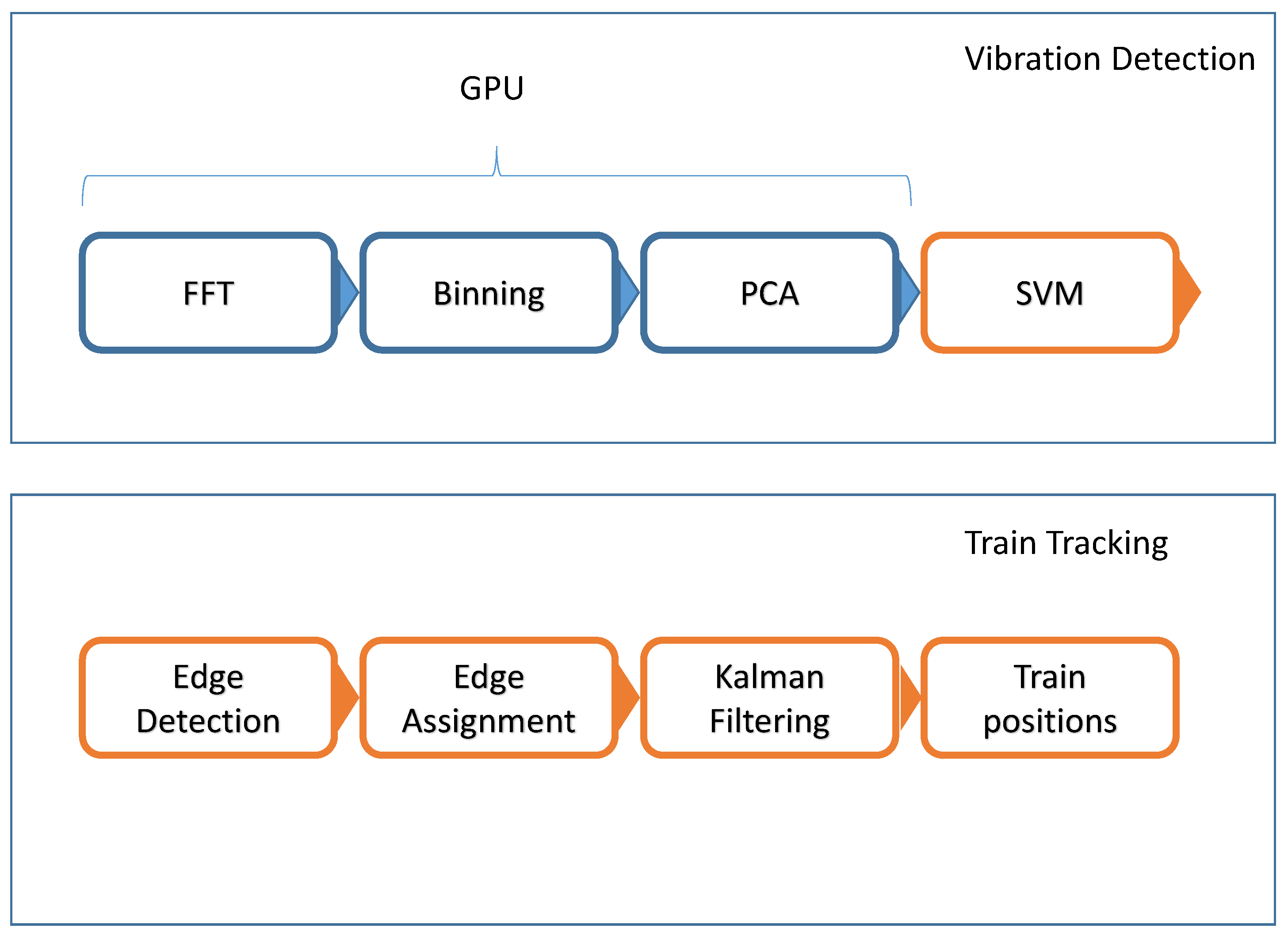
2.3. Vibration Detection

The vibration detection takes as input the raw measurements acquired within one second for all the cable segments along the optical fiber. Given a sampling rate of 2000 Hz and a spatial resolution of $0.68$ $\mathrm{m}$ with a monitored fiber length of 40 km (corresponding to around 60,000 channels), the raw data consist of 2000 × 60,000 samples each second. In the following, we will denote the data matrix containing all the raw measurement data for second i as $M_i$. The result of the vibration detection for this second in time, $v_i$, is a vector of Boolean values of length 60,000, where each element of this vector indicates whether vibration is present at the second i or not for that specific cable segment. Therefore, the vibration detection step corresponds to a data reduction from $M_i$ to $v_i$.

In the following, we will describe the steps we used to perform vibration detection. We use machine learning techniques to decide whether the vector $M_{i,x}$ containing the sensing samples for a given cable segment x and a given second in time i contains vibration or not. The decision is based on the spectral distribution of the raw signal $M_{i,x}$ and is done based on the following steps detailed below. Note that the decision has to be made independently for all the cable segments without any spatial averaging; in the following, therefore, we will describe the procedure for one cable channel.

• Computation of the spectral energy in 10 frequency bins.
• Normalization of the 10 energy values to make them sum up to 1.
• Using Principal Component Analysis (PCA) to reduce the 10 feature values to two feature values.
• Employ a pre-trained Support Vector Machine (SVM) to classify the feature vector of length 2 as vibration or background.

Computation of spectral energy. The energy of the frequencies of the signal $M_{i,x}$ are estimated using the Fast Fourier Transform (FFT). The squared absolute values of the Fourier transformed signal $|M_{i,x}{\left(\xi \right)|}^2$ are then summed up individually for ten bins

$$b_k=\sum _{\xi \in B_k}{\left|M_{i,x}\left(\xi \right)\right|}^2,$$

(1)

where $B_k$ denotes the k-th bin with $k\in \{0,\dots ,9\}$. The frequency bins are linearly spaced and span the frequencies between 10 Hz and 990 Hz.

PCA computation. We use PCA to reduce the number of features from the frequency binning from 10 to 2. This is done by computing two linear combinations of the 10 original features optimally with respect to the variance of the data they can explain. Computationally, this PCA can be represented as a $10\times 2$ matrix. The data used for computing the principal components are from the manually annotated test dataset described in Section 2.2.

SVM classification. SVM classification is used for each cable segment to categorize it as vibration or background for each second in time. The SVM classifier is trained on manually annotated data. We use the SVM implementation of openCV 2.4 with an RBFkernel [17].

2.4. Train Tracking

The train tracking algorithm works on the inputs from the vibration detection and works on a one- second basis. It takes the classification vector $v_i$ and outputs the current positions of the trains present in the signal denoted by $P_j$, where the index j runs through the active trains at the given second i. The train tracking algorithm itself consists of three steps, which we will discuss individually subsequently:

• Extraction of edges from the data.
• Assigning the edges to objects and creating new objects.
• Applying a Kalman filter to smooth the trajectories of all the objects.

Edge Detection. The edge detection is based on a K-means clustering of wavelet responses of the vibration detection vector $v_i$. We use Ricker wavelets of two different widths, namely 128 and 256, cable segments to compute the convolution with the detection vector $v_i$. From both of these convolutions, we extract 512 consecutive values as feature values for the K-means clustering algorithm. A prototypical dataset of vibration detections is used to train the algorithm with four centers which correspond to background, leading edges, trailing edges, and train signal. Note that at this point leading edges are edges that mark the start of a train viewed from the interrogator device, while trailing edges are edges that mark the end of a train. If the train moves towards the interrogator, this leading edge will also be the leading edge of the train; if the train moves away from the interrogator, the leading edge viewed from the interrogator will be the trailing edge of the train. In the following, we will call all these edges detected edges.

Edge Assignment and object creation. The tracking algorithm works internally with two types of objects: tracked edges and tracked trains, which we will denote by $E_i$, $i\in I$ and $P_j$, $j\in J$, respectively. Note that tracked edges are different objects from the detected edges identified in the previous step. In the following, we will describe how the detected edges are assigned to the tracked trains and the tracked edges. This is repeated every second with the corresponding detected edges. Therefore, all the steps described in this paragraph correspond to one given second in time. The algorithm starts to assign detected edges to the list of tracked trains; this is done for detected leading and trailing edges separately. We start by defining cost functions $c_L$ and $c_T$ for a given assignment of an edge e and a Train P by the distance between the edge and the train’s leading edge if e is itself a leading edge and the distance between the edge e and the train’s trailing edge if e itself is a trailing edge. Furthermore, we define a threshold T, which denotes the maximum distance between e and the corresponding edges of the trains, where we still allow an assignment to be made. The formulas for these two cost functions read as

$$\begin{array}{c}\hfill c_L(e,P)=\left\{\begin{array}{cc}|e-P_{\mathrm{Lead}}|\hfill & \mathrm{if}|e-P_{\mathrm{Lead}}|<T\hfill \\ \infty \hfill & \mathrm{if}|e-P_{\mathrm{Lead}}|>T,\hfill \end{array}\right.\end{array}$$

(2)

$$\begin{array}{c}\hfill c_T(e,P)=\left\{\begin{array}{cc}|e-P_{\mathrm{Trail}}|\hfill & \mathrm{if}|e-P_{\mathrm{Trail}}|<T\hfill \\ \infty \hfill & \mathrm{if}|e-P_{\mathrm{Trail}}|>T.\hfill \end{array}\right.\end{array}$$

(3)

Therefore, the two cost functions equal infinity if the detected edge is too far away from the corresponding edge of a given train. If the cost function $c_L(e,P)=\infty$, the edge e will not be assigned to the leading edge of the train P (this is analogous for the function $c_T$ and the trailing edge of P). The assignment problem for a given set of detected leading edges (the assignment works analogously for trailing edges) $e_i,i\in I_e$ to a given set of trains $P_j,j\in I_j$ iteratively finds the minimum in the matrix $C_{i,j}=c_L(e_i,P_j)$ for $i,j$ in the defined index sets. The leading edge and train with the respective indices $i_0$ and $j_0$ corresponding to this minimum, if smaller than ∞, are assigned to each other and the $i_0$-th row and the $j_0$-th column of the cost matrix C are set to ∞. This step is repeated until no more assignments can be made, i.e., the matrix C contains only ∞. The same procedure is then also repeated for the trailing edges of the trains.

After the assignment of leading and trailing edges to the trains, a subset of the originally detected edges has been assigned. The remaining detected edges are then assigned to the currently tracked edges $E_i$ using the same iterative procedure as described for the assignment of edges to trains. We define distance functions analogous to Equation (2), (3), which leads to a definition to an assignment matrix C. With the same greedy iterative algorithm as described above, we can determine the assignments of found edges to tracked edges.

A (possibly empty) subset of the found edges cannot be assigned to a train or to a tracked edge. These edges will become tracked edges in the next time step.

The assignment process described in this section is an approximate greedy approach to the more complex quadratic assignment problem where one tries to find all the assignment index pairs $(i,j)$ such that the corresponding total cost (i.e., the sum of the individual costs for assignments) is minimal. For better readability of the paper, we will not give a rigorous formulation of this optimization problem here since it is computationally not feasible for a real time tracking algorithm.

Kalman filtering. Each train and each tracked edge has an underlying Kalman filter. The tracked edges follow a two-dimensional state-space model consisting of position of the edge and its velocity leading to the following matrices corresponding to a constant velocity model

$$\begin{array}{cc}\hfill F& =\left(\begin{array}{cc}1& 1\\ 0& 1\end{array}\right)\hfill \\ \hfill H& =(1,0),\hfill \end{array}$$

(4)

where F denotes the state transition model, and H denotes the observation model.

The Kalman filter for a tracked train is based on a slightly more involved state-space model. To model a moving train, we propose a four-dimensional state space consisting of leading edge position, trailing edge position, speed, and the length of the train. A measurement at a given time results in the leading and the trailing edge of the train. The resulting constant velocity model leads to the following transition and observation model

$$\begin{array}{cc}\hfill F& =\left(\begin{array}{cccc}1& 0& 1& 0\\ 0& 1& 1& 0\\ 0& 0& 1& 0\\ -1& 1& 0& 0\end{array}\right)\hfill \\ \hfill H& =\left(\begin{array}{cccc}1& 0& 0& 0\\ 0& 1& 0& 0\end{array}\right).\hfill \end{array}$$

(5)

2.5. GPU Computation for Feature Extraction

The computation of the features for the SVM classification needs to be able to process the raw data matrix $M_i$ containing the data for second i in time and all the channels along the optical fiber. As mentioned above, for a typical setup of 40 km monitoring length and a sampling rate of 2000 Hz this leads to a data matrix of dimensions in the order of 2000 × 60,000. In the case of a Helios DAS interrogator device, the data format is unsigned int 16, which leads to a data rate of 228 MB/s. We then have to cast these data to a float datatype because the first step involves a Fourier transform that doubles the data rate as we use 32 bit float values. This Fourier transform computation has to be done for all 60,000 cable segments in parallel. The highly parallelizable nature of these computations makes general purpose GPUs (GPGPU) highly suitable for the task. The same holds true for the PCA feature reduction, which has to be applied for each cable segment individually. The SVM classifier is not available with GPU acceleration; therefore, the reduced features are downloaded to the CPU before classification. A flow chart of the complete algorithm is depicted in Figure 1.

3. Results

This section is devoted to the results. We will start to discuss the results for the different stages of the tracking algorithm and then present the results for two long term recordings, as well as tracking accuracy results for a short-term recording where a ground truth of the train positions was available.

3.1. Train Tracking Stages

To perform the vibration detection, we first annotated vibrations in a recorded raw data file individually for the two different track conditions. These ground truth data are then used to train the PCA for feature reduction and the SVM for classification. An illustration of the vibration detection can be found in Figure 2.

The first step of the tracking algorithm is the edge detection. In Figure 3, we give an example of the result of the edge detection from the first 35 s of the dataset shown in Figure 2. After the edge detection, the assignment and Kalman filtering are performed. For the same example dataset, we show the tracking result in Figure 4.

3.2. Evaluation of Tracking Accuracy

For two datasets encompassing around 3000 $\mathrm{s}$ of recording each, we have available ground truth positional data for two points along the track. The recording was done on an open track with the cable installed in a cable trench. The available ground truth is accurate to one second in time, which leads to an accuracy of around 30 to 40 m considering that this is the speed the objects move on the test infrastructure. The tracking errors in meters can be found in

Table 2. Summarized performance of tracking algorithm for the two two short term recordings for single trains. Given that the ground truth and the tracking are both accurate down to one second, the evaluation is accurate down to 2 s. Considering the train speed, which is around 30–40 m/s, the errors are in the expected range.

Train ID	Error Signal 1 [m]	Error Signal 2 [m]
23468	49.64	44.20
29515	48.96	1.36
2330	51.68	38.76
73	79.56	37.40
23488	71.40	23.12
29535	44.88	17.00
23508	31.28	86.36
29555	31.28	19.72
103	64.60	57.12
90093	43.52	39.44
23528	49.64	64.60
29575	2.04	61.20
Average	47.37	40.86

. The tracking error is in the range of 40 $\mathrm{m}$, which is in the range of the available ground truth considering that both, the ground truth and the tracking algorithm, work on a one second basis that leads to a maximally two-second difference between the two systems, and the trains move at a speed of 30–40 m/s.

3.3. Evaluation of Tracking Reliability

In this section, we will evaluate the tracking reliability based on two long term recording results. One is done in a tunnel where only one tube in one direction has been measured. The second test site is a standard track with the cable mounted directly on the rail. To evaluate the number of correctly tracked trains without the availability of ground truth from an alternative tracking system, the following steps were taken:

• Identify the tracks that do not end at the end of the monitored cable section or in a station as potential tracking errors.
• Exclude trains that stop on the open track as in that case the train ID is lost based on visual evaluation.
• Exclude artifact tracks based on visual evaluation.
• Count the total number of train tracks and the number of excluded tracks.

We collect the respective numbers of the correct and lost train tracks for two different test sites, where we were conducting long term measurements in

Table 3. Summarized performance of tracking algorithm for the two monitored test sites.

	Test Site 1	Test Site 2
Cable stretch observed (meters)	13,600–25,900	0–8840
Cable stretch observed (segments)	20,000–38,000	0–13,000
Number of hours observed	477	538
Cable installation method	Cable trench in tunnel	Cable attached to rail on open track
Number of tracks	2174	1071
Number of correct tracks	2141	1059
% of correct trains	98%	99%

. In the following subsections, we will describe the specific results for the two test sites.

3.3.1. Test Site 1: Tunnel

The monitored section of the cable in the tunnel is from 13,600 m to 25,900 m relative distance from the interrogator device; therefore, we observe a long stretch of cable. This analysis shows that we reach 98% of correct tracks, respectively, for the two evaluated cable lengths. In this test site, no artifact tracks due to non-train-related noise was observed, meaning that the two percent incorrect tracks are attributed to lost tracks.

3.3.2. Test Site 2: Open track

This test site consists of an open track with a cable that is directly mounted on the rail, which leads to a very different scenario from the first test site. In our test period, we were not observing any lost tracks of moving trains on the open track. However, due to the cable installation method, we observed a higher amount of noise in the signal, which leads to a number of false positive detections of trains during the evaluation period. Of the 1071 total tracks, we found 12 to be artifacts, which leads to a total of 99% correct tracks. Generally, mounting the optical cable directly on the rail leads to more noise in the signal that is not caused by trains. This is not surprising since such a cable is exposed to natural elements, such as wind and rain. Furthermore, we observed that certain sections of the cable seem to be coupled, meaning that if a train enters such a section, all the cable segments in that section will vibrate. An illustration of this phenomenon, as well as of the increased noise in the signal, can be found in Figure 5. The coupling of fiber segments leads to decreased accuracy in estimating the train length because the detected leading and trailing edge do not coincide with the start and end of the train but, rather, with the start and end of the coupled segments.

3.3.3. Comparison with the Literature

The goal of this section is to discuss the presented results in comparison to the approaches discussed in the literature. The main difference between the algorithms described in the literature and our approach is the flexibility of our method through the use of machine learning.

The papers of Timofeev et al. [12,13] describe an energy based train vibration detection. According to our experience, this approach is not feasible for long stretches of monitored fiber with the recording device we used. The paper does not mention the validation data used for drawing the conclusions, nor does it mention a tracking algorithm. The accuracy of the proposed method with respect to positional accuracy is reported at 15 $\mathrm{m}$. In comparison, we did not have a ground truth available with such a high accuracy.

The paper of Peng et al. [14] describes an algorithm which uses a relative variance for vibration detection. The validation data for the method are two trains recorded over 400 $\mathrm{s}$. The paper does not mention any accuracy measurements for the proposed method, nor do the authors mention which tracking algorithm is used.

The earlier papers of some of the authors of this contribution [15,16] describe a similar algorithm with some important difference. The earlier versions of the algorithm used a filtering over time which introduced a delay. This has been changed in this contribution to Kalman filtering avoiding a time lag of the method. Furthermore, the edge detection has been refined to be more flexible, which is especially important for rail foot cables.

We can conclude that this is, to our knowledge, the most extensive study done on railway monitoring using DAS. In comparison to the other literature, we used flexible methods that allow for efficient re-calibration for different track conditions.

4. Discussion

In this paper, we presented a real-time train tracking algorithm that runs on the basis of one-second signals without delay. The algorithm is based on two main steps, i.e., the detection of vibrations and the tracking of trains in the signal. The performance of the algorithm was evaluated on two test sites, where one was in a tunnel with a standard cable trench and the other one was on an open track with the cable attached directly to the rail. In the tunnel, we measured a long distance which lead to occasionally lost tracks, especially on a stretch where the cable installation was sub-optimal for transferring vibrations from the train to the cable. On the open track with the cable mounted directly to the rail, we did not observe lost tracks during the test period, which is due to strong signals, because the observed cable length was considerably shorter than in the tunnel. Due to the increased noise with the cable installation method, we observed several artifact train tracks. Nevertheless, for both evaluated tracks we reached accurate tracks in more than 98% of the cases. We conclude from the results that the installation in a cable trench is advantageous for train tracking with a DAS system.

For two shorter recordings, we presented the positional error, which was around 40 $\mathrm{m}$, which was also in the range of the available ground truth. For more accurate evaluations of the positional accuracy of the tracking, it would be important to get better ground truth data and perform a highly accurate calibration of the fiber cable.

For application in the railway sector, DAS shows great potential, especially when combined with other sensors for redundancy. In future research, we will evaluate methods for fusing different sensor modalities to increase the robustness of the tracking.

References

1. Gao, S.; Dong, H.; Ning, B.; Zhang, Q. Cooperative Prescribed Performance Tracking Control for Multiple High-Speed Trains in Moving Block Signaling System. IEEE Trans. Intell. Transp. Syst. 2019, 20, 2740–2749. [Google Scholar] [CrossRef]
2. Hill, R.; Bond, L. Modelling moving-block railway signalling systems using discrete-event simulation. In Proceedings of the 1995 IEEE/ASME Joint Railroad Conference, Baltimore, MD, USA, 4–6 April 1995; pp. 105–111. [Google Scholar] [CrossRef]
3. Williams, C. The next ETCS Level? In Proceedings of the 2016 IEEE International Conference on Intelligent Rail Transportation (ICIRT), Birmingham, UK, 23–25 August 2016; pp. 75–79. [Google Scholar] [CrossRef]
4. Albrecht, T.; Luddecke, K.; Zimmermann, J. A precise and reliable train positioning system and its use for automation of train operation. In Proceedings of the 2013 IEEE International Conference on Intelligent Rail Transportation Proceedings, Beijing, China, 30 August–1 September 2013; pp. 134–139. [Google Scholar] [CrossRef]
5. Champavère, A. New OTDR Measurement and Monitoring Techniques. In Proceedings of the Optical Fiber Communication Conference (OFC 2014), San Francisco, CA, USA, 9–13 March 2014; p. W3D.1. [Google Scholar] [CrossRef]
6. Dean, T.; Hartog, A.; Papp, B.; Frignet, B. Fibre optic based vibration sensing: Nature of the measurement. In Proceedings of the 3rd EAGE Workshop on Borehole Geophysics, Athens, Greece, 19–22 April 2015. [Google Scholar]
7. Bao, X.; Chen, L. Recent Progress in Distributed Fiber Optic Sensors. Sensors 2012, 12, 8601–8639. [Google Scholar] [CrossRef] [PubMed] [Green Version]
8. Baldwin, C.S. Brief history of fiber optic sensing in the oil field industry. In Proceedings of the Fiber Optic Sensors and Applications XI, Baltimore, MD, USA, 5–9 May 2014; p. 909803. [Google Scholar] [CrossRef]
9. Juarez, J.C.; Maier, E.W.; Choi, K.N.; Taylor, H.F. Distributed fiber-optic intrusion sensor system. J. Lightwave Technol. 2005, 23, 2081. [Google Scholar] [CrossRef]
10. Peng, F.; Wu, H.; Jia, X.H.; Rao, Y.J.; Wang, Z.N.; Peng, Z.P. Ultra-long high-sensitivity Φ-OTDR for high spatial resolution intrusion detection of pipelines. Opt. Exp. 2014, 22, 13804–13810. [Google Scholar] [CrossRef] [PubMed]
11. Chen, C.; Chen, R.; Wei, F.; Wu, D. Experimental and application of spiral distributed optical fiber sensors based on OTDR. In Proceedings of the 2011 International Conference on Electric Information and Control Engineering, Wuhan, China, 15–17 April 2011; pp. 5905–5909. [Google Scholar] [CrossRef]
12. Timofeev, A.V.; Egorov, D.V.; Denisov, V.M. The Rail Traffic Management with Usage of C-OTDR Monitoring Systems. World Acad. Sci. Eng. Technol. Int. J. Comput. Electr. Autom. Control Inf. Eng. 2015, 9, 1492–1495. [Google Scholar]
13. Timofeev, A.V. Monitoring the Railways by Means of C-OTDR Technology. Int. J. Mech. Aerosp. Ind. Mech. Eng. 2015, 9, 634–637. [Google Scholar]
14. Peng, F.; Duan, N.; Rao, Y.J.; Li, J. Real-Time Position and Speed Monitoring of Trains Using Phase-Sensitive OTDR. Photonics Technol. Lett. 2014, 26, 2055–2057. [Google Scholar] [CrossRef]
15. Papp, A.; Wiesmeyr, C.; Litzenberger, M.; Garn, H.; Kropatsch, W. A real-time algorithm for train position monitoring using optical time-domain reflectometry. In Proceedings of the 2016 IEEE International Conference on Intelligent Rail Transportation (ICIRT), Birmingham, UK, 23–25 August 2016; pp. 89–93. [Google Scholar] [CrossRef]
16. Papp, A.; Wiesmeyr, C.; Litzenberger, M.; Garn, H.; Kropatsch, W. Train Detection and Tracking in Optical Time Domain Reflectometry (OTDR) Signals. In Proceedings of the German Conference on Pattern Recognition, Hannover, Germany, 12–15 September 2016; pp. 320–331. [Google Scholar]
17. Bradski, G. The OpenCV Library. Dr. Dobb’s J. Softw. Tools 2000. Available online: https://github.com/opencv/opencv/wiki/CiteOpenCV (accessed on 7 January 2020).
Figure 1. Flow chart of the algorithm. The top box describes the steps of the vibration detection (steps on the GPU are in blue); the bottom box describes the steps of the train tracking. FFT = Fast Fourier Transform; PCA = Principal Component Analysis; SVM = Support Vector Machine.
Applsci 10 00448 g001
Figure 2. Left: Raw subsampled signal for visualization. Right: Result of the vibration detection where white pixels indicate vibration and black pixels indicate background. The gaps in the train tracks occur when a train stops since an electric train that is not moving does not emit any vibrations and is, therefore, not visible usind a Distributed Acoustic Sensing (DAS) system.
Applsci 10 00448 g002
Figure 3. Leading and trailing edge of the object in blue and orange, respectively, plotted over the vibration detection results in black and white; note that the depicted signal consists of the first 35 s of the signal shown in Figure 2.
Applsci 10 00448 g003
Figure 4. Train tracking result for an example dataset (colored lines), detection result in black and white; note that the depicted signal is the same as in Figure 2.
Applsci 10 00448 g004
Figure 5. Top Left: Subsampled signal through band energy calculation. Top Right: Train Detection result for a train on test site 2; the green boxes indicate coupled cable segments; the background without train shows increased noise. Bottom: False positive train track due to false positive vibration detections.
Applsci 10 00448 g005