Synthesis of Normal Heart Sounds Using Generative Adversarial Networks and Empirical Wavelet Transform

Abstract

Currently, there are many works in the literature focused on the analysis of heart sounds, specifically on the development of intelligent systems for the classification of normal and abnormal heart sounds. However, the available heart sound databases are not yet large enough to train generalized machine learning models. Therefore, there is interest in the development of algorithms capable of generating heart sounds that could augment current databases. In this article, we propose a model based on generative adversary networks (GANs) to generate normal synthetic heart sounds. Additionally, a denoising algorithm is implemented using the empirical wavelet transform (EWT), allowing a decrease in the number of epochs and the computational cost that the GAN model requires. A distortion metric (mel–cepstral distortion) was used to objectively assess the quality of synthetic heart sounds. The proposed method was favorably compared with a mathematical model that is based on the morphology of the phonocardiography (PCG) signal published as the state of the art. Additionally, different heart sound classification models proposed as state-of-the-art were also used to test the performance of such models when the GAN-generated synthetic signals were used as test dataset. In this experiment, good accuracy results were obtained with most of the implemented models, suggesting that the GAN-generated sounds correctly capture the characteristics of natural heart sounds.

1. Introduction

Cardiovascular diseases are one of the leading causes of death in the world. According to recent reports from the World Health Organization and the American Heart Association, more than 17 million people die each year from these diseases. Most of these deaths (about 80%) occur in low- and middle-income countries [1,2]. Tobacco use, unhealthy eating, and lack of physical activity are the main causes of heart disease [1].

Currently, there are sophisticated equipment and tests for diagnosing heart disease, such as: electrocardiogram, holter monitoring, echocardiogram, stress test, cardiac catheterization, computed tomography scan, and magnetic resonance imaging [3]. However, most of this equipment is very expensive, and must be used by specialized technicians and medical doctors, which limits its availability in rural and urban areas that do not have the necessary financial resources [4]. Therefore, even today, it is common in such scenarios for non-specialized medical personnel to rely on basic auscultation with an stethoscope as a primary screening tool for the detection of many cardiac abnormalities and heart diseases [5]. However, to be effective, this method requires a sufficiently trained ear to identify cardiac conditions. Unfortunately, the literature suggests that in recent years such auscultation training has been in decline [6,7,8].

This situation has motivated the development of computer classification models to support the identification of normal and abnormal heart sounds by non-specialized health professionals. To date, many investigations related to the analysis and synthesis of heart sounds (HSs) have been published, obtaining good results especially in the classification of normal and abnormal heart sounds [9,10,11,12,13,14,15,16,17,18,19,20,21,22,23,24,25].

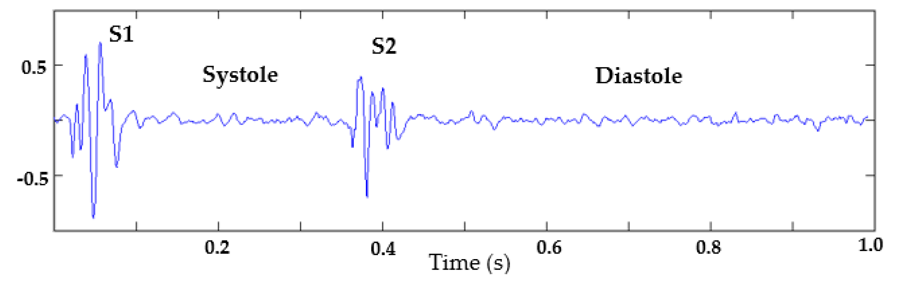
Heart sounds are closely related to both, the vibration of the entire myocardial structure and the vibration of the heart valves during closure and opening. A recording of heart sounds is composed of series of cardiac cycles. A normal cardiac cycle, as shown in Figure 1, is composed by the S1 sound (generated by the closing of the atrioventricular valve), the S2 sound (generated by the closing of the semilunar valve), the systole (range between S1 and S2), and the diastole (range included between S2 and S1 of the next cycle) [26]. Abnormalities are represented by murmurs that usually occur in the systolic or diastolic interval [27]. Health professionals use different attributes of heart murmurs for their classification, the most common are: timing, cadence, duration, pitch, and shape of the murmur [28,29]. Therefore the examiner must have an ear sufficiently trained to identify each of these attributes.

Despite the amount of work related to the classification of heart sounds, it is still difficult to statistically evaluate the robustness of these algorithms, since the number of samples used in training is not sufficient to guarantee a generalized model. Similarly, there have been no significant advances in the classification of specific types of heart murmurs, due to the limited availability of corresponding labels in current public databases [30,31]. In this sense, having a model for the generation of synthetic sounds, capable of outputting varied synthetic heart sounds indistinguishable from natural ones by medical personnel, could be used to augment existing databases for training robust machine learning models. However, heart sound signals are highly non-stationary, and their level of complexity makes obtaining good generative models very challenging.

In the literature, there are several publications related to the generation of synthetic heart sounds [16,17,18,19,20,21,22,23,24,25]. All these works are based on mathematical models to generate the S1 and S2 sections of a cardiac cycle. On the other hand, the systolic and diastolic intervals of the cardiac cycle are not adequately modeled, and as a result, do not present the variability recorded in natural normal heart sounds. Therefore, these synthetic models are not suitable to train HS classification models. Additionally, a basic time–frequency analysis of these synthetic signals shows that they are very different from natural signals.

Table 1. Timeline of methods for the generation of synthetic heart sounds.

Year	Author	Previous Method
1992	Tang et al. [16]	Exponentially damped sinusoidal model
1995	Trang et al. [17]	S1 and S2 as transient–linear chirp signals
1998	Zhang et al. [18]	Sum of Gaussian-modulated sinusoidal
2000	Xu et al. [19]	S1 and S2 as transient–nonlinear chirp signal
2009	Toncharoen et al. [20]	A heart-sound-like chaotic attractor
2011	Almasi et al. [21]	A dynamical model based in electrocardiogram (ECG) signal
2012	Tao et al. [22]	Amplitude and width modification of S1 and S2 sounds from real heart sounds, and combining them with noise
2013	Jablouna et al. [23]	Coupled ordinary differential equations
2018	Saederup [24]	Estimation of the second heart-sound split using windowed sinusoidal models
2018	Joseph et al. [25]	Sum of almost periodically recurring deterministic “wavelets”; S1 and S2 are modeled by two sinusoidal pulses of Gaussian modulation.

presents a comparison of the different heart sound generative methods found in the Web of Science, Scopus, and IEEE Xplore databases.

On the other hand, in recent years there have been great advances in the synthesis of audio, mainly speech, using machine learning techniques, specifically with deep learning. In

Table 2. Previous methods for generation of synthetic audio.

Year	Author	Previous Method	Synthetic Signal
2015	van den Oord et al. [32]	WaveNet: Probabilistic and autoregressive model based on deep neural networks (DNNs)	Music; text-to-speech
2017	Engel et al. [33]	WaveNet and autoenconders	Musical notes
2017	Bollepalli et al. [34]	Generative adversarial network (GAN)	Glottal waveform
2018	Biagetti et al. [35]	Hidden Markov model	Text-to-speech
2019	Donahue et al. [36]	WaveGAN: GANs unsupervised	Intelligible words

, several proposed methods to improve audio synthesis are presented.

According to the limitations presented in the currently proposed models for the generation of synthetic heart sounds, and taking into account the significant advances in voice synthesis using deep learning methods, in this work we propose a model based on generative adversarial networks (GANs) to generate only normal heart sounds that can be used to train machine learning models. This article is organized as follows: Section 2 presents a definition of the GAN architecture; in Section 3, the proposed method is described; Section 4 presents experimental results, using mel–cepstral distortion (MCD) and heart sound classification models; finally, the conclusions and discussions of the proposed work and experiments are presented in Section 5.

2. Generative Adversarial Networks (GANs)

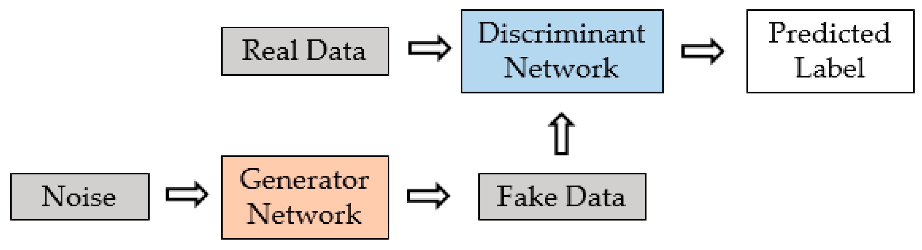
Generative adversarial networks (GANs) are architectures of deep neural networks widely used in the generation of synthetic images [37]. This architecture is composed of two neural networks that face each other, called the generator and discriminator [38]. In Figure 2, a general diagram of a GAN architecture is presented.

The generator (counterfeiter) needs to learn to create data in such a way that the discriminator can no longer distinguish it as false. The competition between these two networks is what improves their knowledge, until the generator manages to create realistic data.

As a result, the discriminator must be able to correctly classify the data generated by the generator as real or false. This means that their weights are updated to minimize the probability that any false data will be classified as belonging to the actual data set. On the other hand, the generator is trained to trick the discriminator by generating data as realistically as possible, which means that the weights of the generator are optimized to maximize the probability that the false data it generates will be classified as real by the discriminator [38].

The generator is an inverse convolutional network—that is, it takes a random noise vector and converts it into an image—unlike the discriminator, which takes an image and samples it to produce a probability. In other words, the discriminator (D) and generator (G) play the following two-player min/max game with value function L(G, D), as described in Equation (1):

$$\underset{G}{\min }\underset{D}{\max }L\left(D,G\right)={\mathbb{E}}_{x\sim {\rho }_{data}\left(x\right)}\left[\log D\left(x\right)\right]+{\mathbb{E}}_{z\sim {\rho }_{data}\left(z\right)}\left[\log (1-D\left(G\left(z\right)\right)\right]$$

(1)

where D(x) represents the probability that x is estimated by the discriminator, z represents the input of random variables from the generator, and ${\rho }_{data}\left(x\right)$ and ${\rho }_{data}\left(z\right)$ denote the data distribution and the distribution of samples from the generator, respectively.

After several training steps, if the generator and the discriminator have sufficient capacity (if the networks can approach the objective functions), they will reach a point where both can no longer improve. At this point, the generator generates realistic synthetic data, and the discriminator cannot differentiate between the two input types.

3. Proposed Method

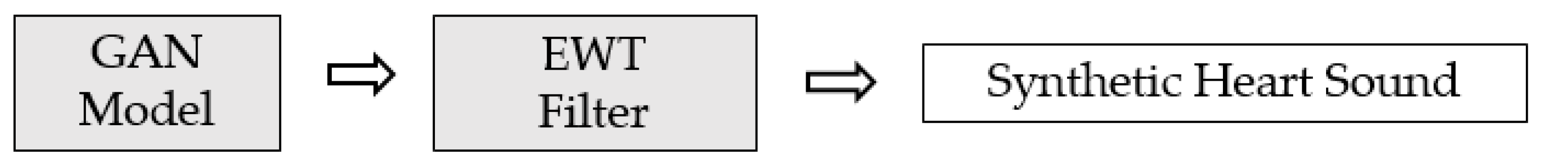
The proposed method is made up of two main stages, as shown in Figure 3. The first stage consists of the implementation of a GAN architecture to generate a synthetic heart sound, and the second stage is in charge of reducing the noise of the synthetic signal using an empirical wavelet transform (EWT). This last stage consists of a post-processing applied to the signal generated by the GAN, in order to attenuate the noise level. Therefore, it makes it possible to reduce the number of epochs (and consequently the computational cost) required to train the GAN until obtaining a low-noise output signal.

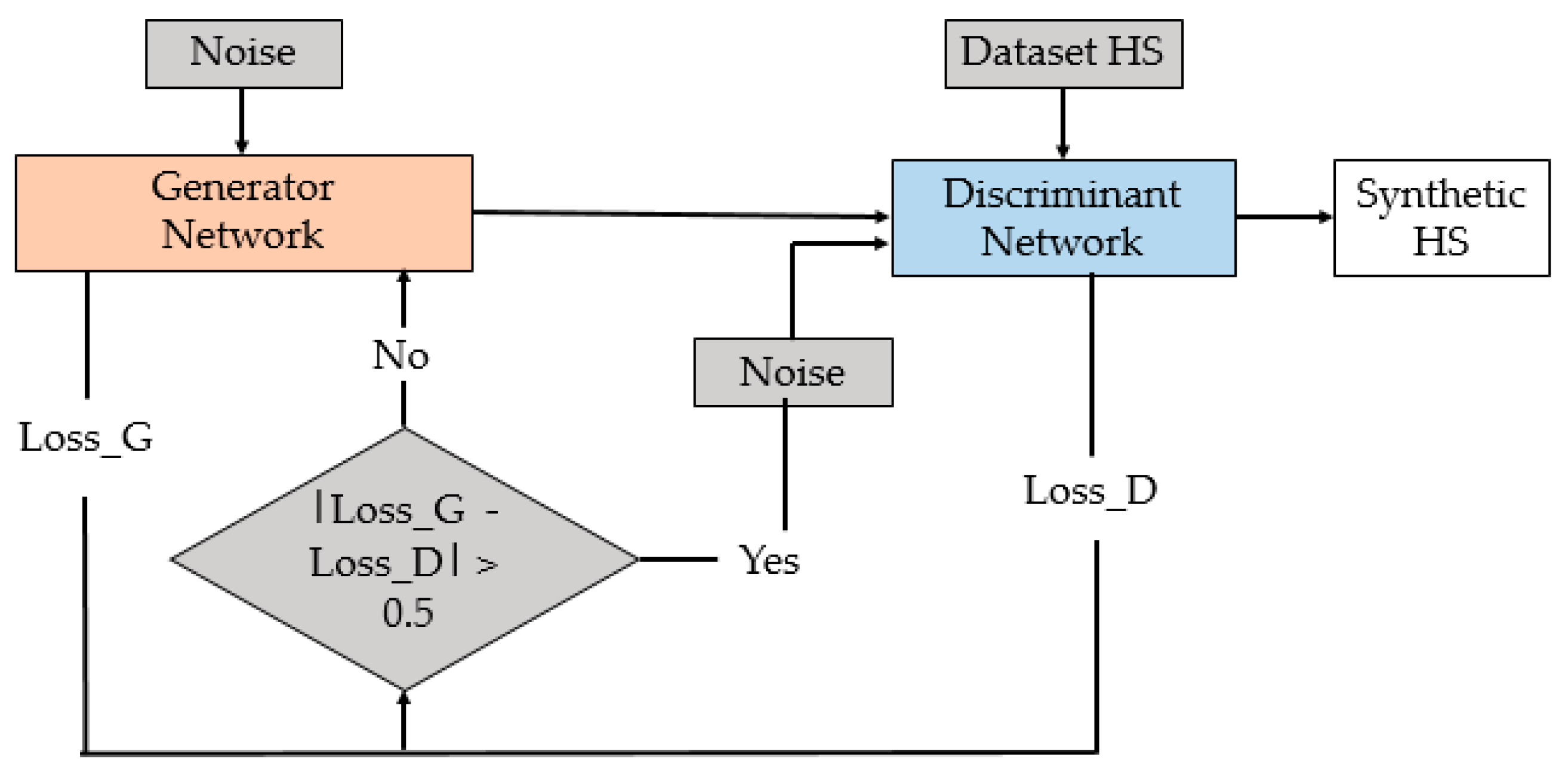
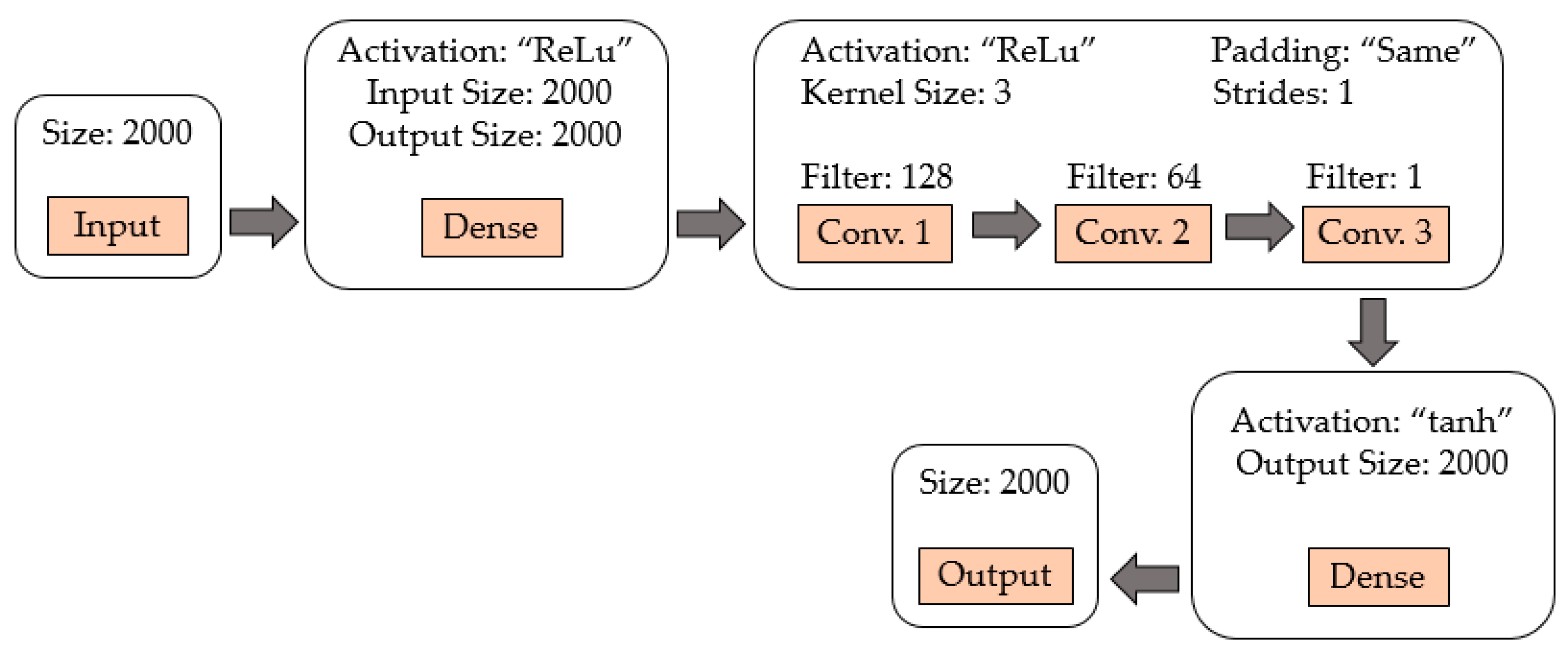
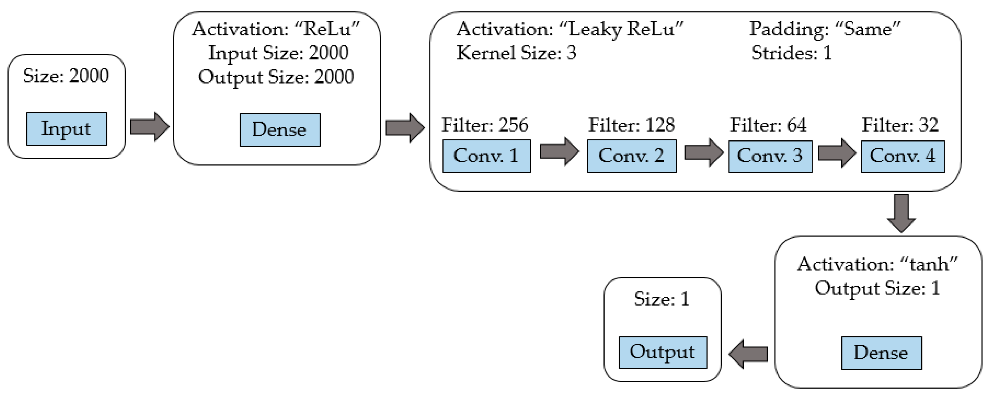
Figure 4 shows the diagram of the implemented GAN architecture, and each of its components is described below.

• Noise: a gaussian noise with a size of 2000 samples is used as input to the generator. The mean and standard deviation of the noise’s distribution are 0 and 1, respectively;
• Generator model: Figure 5 shows a diagram of the generating network, and the hyperparameters of each layer are specified. It begins with a dense layer with ReLu activation function, followed by three convolutional layers with filters of size 128, 64, and 1, respectively; each of these layers have ReLu activation function, a kernel size of 3, and a stride of 1. Finally, there is a dense layer with a tanh activation function. The padding parameter is set to “same” to maintain the same data dimension in the input and output of the convolutional layer;
• Discriminator model: Figure 6 shows a diagram of the discriminator network. It begins with a dense layer with ReLu activation function, followed by four convolutional layers with filters of size 256, 128, 64, and 32, respectively; each of these layers uses Leaky ReLu activation function, a kernel size of 3, and a stride of 1; additionally, between each convolution layer there is a dropout of 0.25. Finally, there is a dense layer with a tanh activation function. The padding parameter is set to “same” to maintain the same data dimension in the input and output of the convolutional layer;
• Dataset of heart sounds: 100 normal heart sounds obtained from the Physionet database [30] were used, with a sampling frequency of 2 KHz and 1 s of duration. For this dataset, those signals with a similar heart rate were selected—that is, all signals have a similar systolic and diastolic interval duration;
• Optimization: the Adam optimizer was used, since it is one of the best performers in this type of architecture. A learning rate of 0.0002 and a beta of 0.3 were set;
• Loss function: a binary, cross-entropy function weas used in this work. This function computes the cross-entropy loss between true labels and predicted labels.

Subsequently, the difference between generator and discriminator losses was analyzed. If this difference was greater than 0.5, the input data to the discriminator was switched to a Gaussian noise with a mean of 0 and standard deviation of 1, and not the generator output as it was otherwise. With this method, a convergence in the loss functions of the generator and discriminator could be achieved.

As mentioned before, the second stage of the proposed method aims to reduce the noise level of the synthetic signal generated by the GAN model. It is understood that as the number of epochs in the training of the generator and discriminator models increases, the noise of the synthetic signal is attenuated; however, it requires many epochs, and in turn, a long computation time [39]. Therefore, in order to reduce the number of GAN training epochs required to generate synthetic signals with acceptable noise levels, it was decided to introduce a post-processing stage using the algorithm proposed in [40], called empirical wavelet transform (EWT). The EWT allows the extraction of different components of a signal by designing an appropriate filter bank. The theory of the EWT algorithm is described in detail in [40]. This algorithm has been used in different signal processing applications [41,42,43]. In [9], a modified version of this algorithm was used as a pre-processing stage in the analysis of heart sounds. Its implementation is described in more detail in [9]. In this work, it was decided to use as a reference the method proposed in [9] to reduce the noise of the synthetic signal.

Taking into account that the frequency range of the S1 and S2 sounds is between 20–200 Hz [44], it was decided to modify the edge selection method that determines the number of components for the EWT algorithm. The signal is then broken down into two frequency bands: the first component corresponds to the frequency range between 0–200 Hz, while the second component corresponds to frequencies over 200 Hz. Therefore, in this work, the signal corresponding to the first component is used.

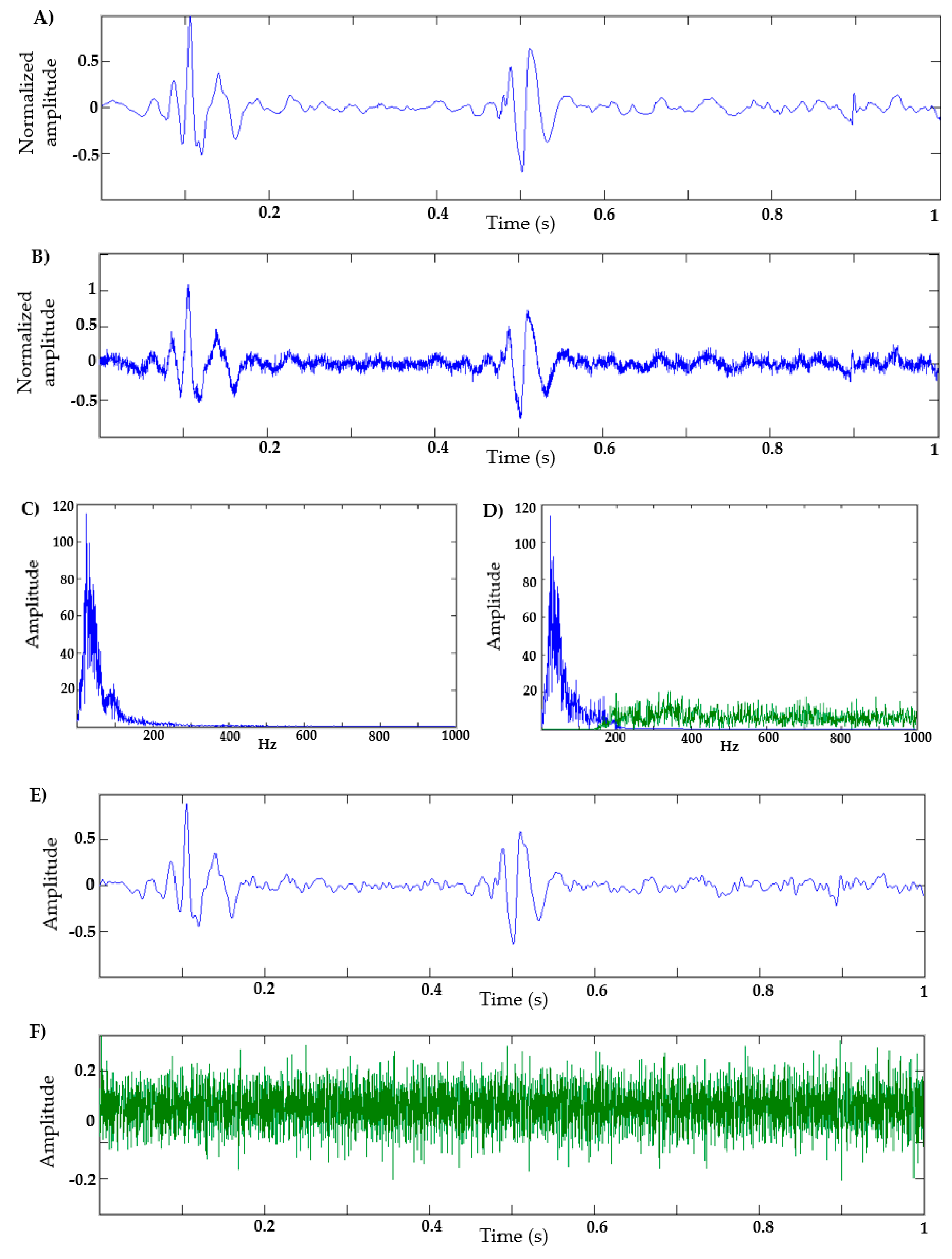
Taking into account that the input of the GAN model is a Gaussian noise, and in turn, the output of the model during the first epochs of training is expected to be a signal mixed with Gaussian noise, it was decided to do a test using a real heart signal mixed with Gaussian noise to evaluate the performance of the proposed EWT filter on signals with the same expected characteristics of the generator’s output. Figure 7A,B shows, respectively, a real heart sound and the same heart sound mixed with low-amplitude Gaussian noise, while Figure 7C,D shows their respective Fourier transforms (FFTs). In this last figure, the frequency of the components between 0 and 200 Hz can be seen in blue, and the frequency of components above 200 Hz caused by the Gaussian noise are in green. The signal shown in Figure 7B was then used as an input example to the proposed EWT algorithm to illustrate its de-noising action. Figure 7D shows the two frequency bands extracted with EWT using the FFT, while Figure 7E,F shows the two components extracted from the noisy signal in the time domain. As can be seen, the signal obtained in Figure 7E presents a lower noise level, and is comparable with the original cardiac signal shown in Figure 7A.

4. Experiments and Results

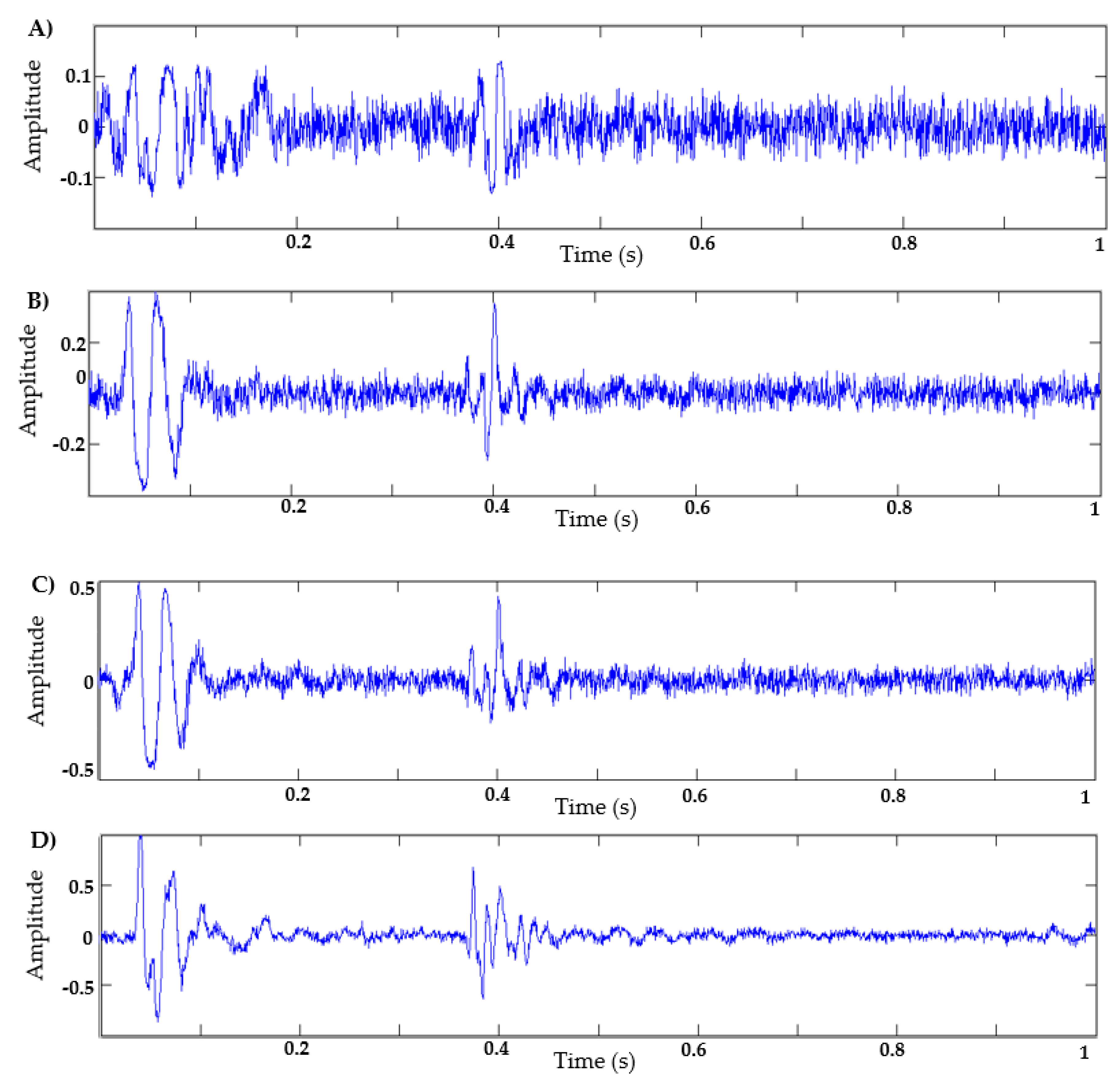
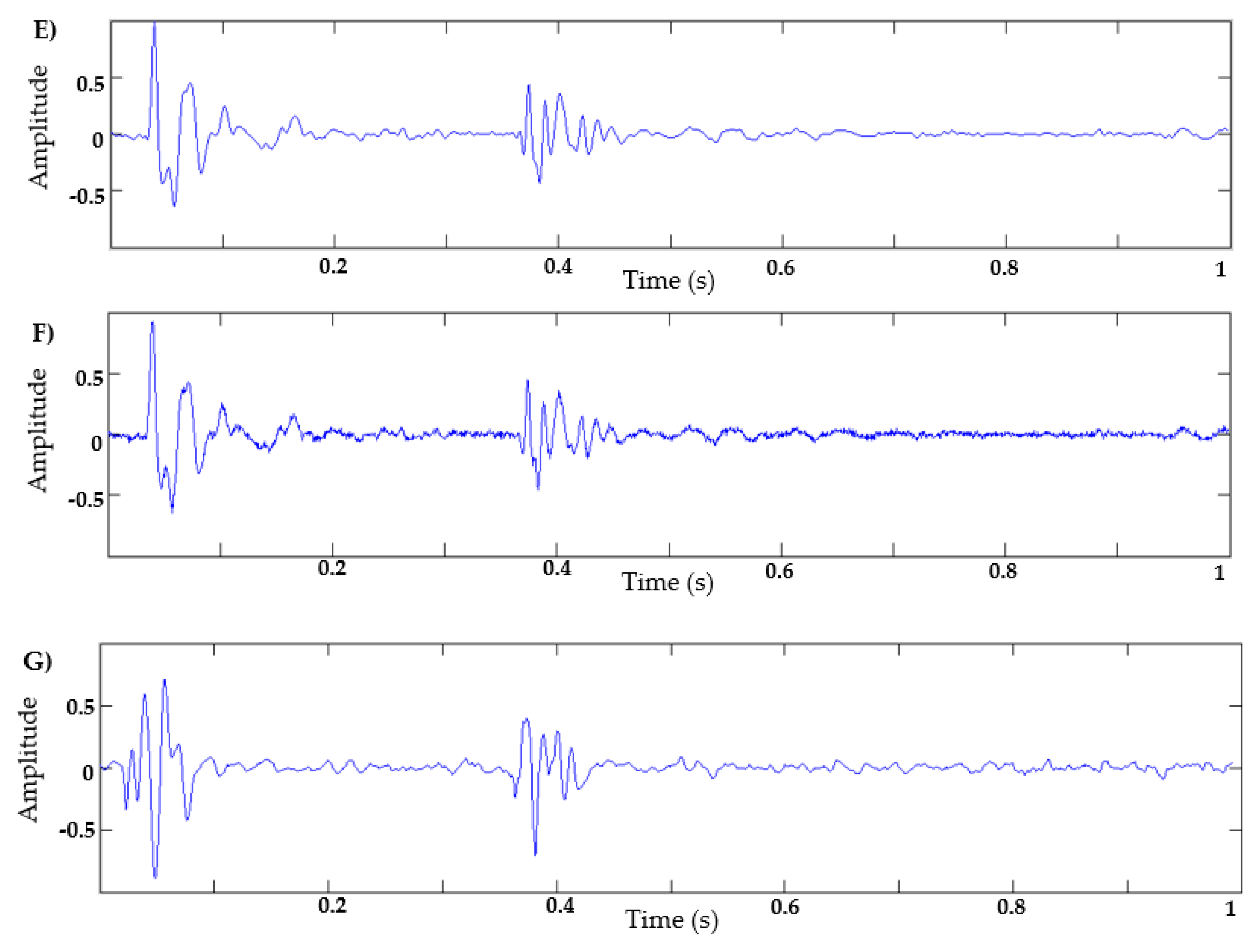
The proposed GAN model was trained for a total of 2000 epochs. Figure 8 shows sample output signals generated at different epochs. As can be observed, as the epochs increase, the signals present a more realistic form. In this work, the EWT filter is a post-processing stage that is applied to the synthetic signal generated with 2000 training epochs, in order to reduce the noise level of the generator output. Therefore, the EWT filter is not part of the training loop for the GAN. This number of epochs was determined after observing the synthetic signals obtained at different training points (from 100 epochs to 12,000 epochs). It was observed that from 2000 epochs, the synthetic signal has a shape very similar to a natural signal, but with a relatively high noise level, as shown in Figure 8E. Therefore, it was decided to generate the synthetic signals up to 2000 epochs, and subsequently apply the proposed EWT algorithm. Figure 8F,G shows the results of a synthetic signal generated with 12,000 training epochs without applying an EWT algorithm or a natural signal, respectively.

In this work, a comparison is made between the proposed method and a mathematical model proposed in [21], in order to determine which method generates a cardiac signal realistic enough to be used by a classification model. The mathematical method [21] was inspired by a dynamic model that generates a synthetic electrocardiographic signal, as described [45]. Therefore, this model is based on the morphology of the phonocardiographic signal, and has been used as a reference in other proposed methods [23]. The equation for the reference model [21] is described below:

$$\dot{\dot{z}=-{\displaystyle \sum }_{i\in \left\{S{1}^{- }S{1}^{+}S{2}^{-}S{2}^{+}\right\}}\left(\frac{{\alpha }_i}{{\sigma }_i}\left(\theta -{\mu }_i\right)e^{\left(\frac{{\left(\theta -{\mu }_i\right)}^2}{2{\sigma }_i^2}\right)}\cos \left(2\pi f_i\theta -{\phi }_i\right)+2\pi {\alpha }_i{f}_i{e}^{\left(\frac{{\left(\theta -{\mu }_i\right)}^2}{2{\sigma }_i^2}\right)}\sin \left(2\pi f_i\theta -{\phi }_i\right)\right)}$$

(2)

where ${\alpha }_i$, ${\mu }_i$, and ${\sigma }_i$ are the parameters of amplitude, center, and width of the Gaussian terms, respectively; $f_i$ and ${\phi }_i$ are the frequency and the phase shift of the sinusoidal terms, respectively; and $\theta$ is an independent parameter in radians that varies in the range -π, π for each beat. The parameters used by the authors in [21] are summarized in

Table 3. Parameters used in [21] to generate normal heart sounds.

Index (i)	S1 (-)	S1 (+)	S2 (-)	S2 (+)
${\alpha }_i$	0.4250	0.6875	0.5575	0.4775
${\mu }_i$ (radians)	π/12	3π/19	3π/4	7π/9
${\sigma }_i$	0.1090	0.0816	0.0723	0.1060
$f_i$ (Hz)	10.484	11.874	11.316	10.882
${\phi }_i$ (radians)	3π/4	9π/11	7π/8	3π/4

.

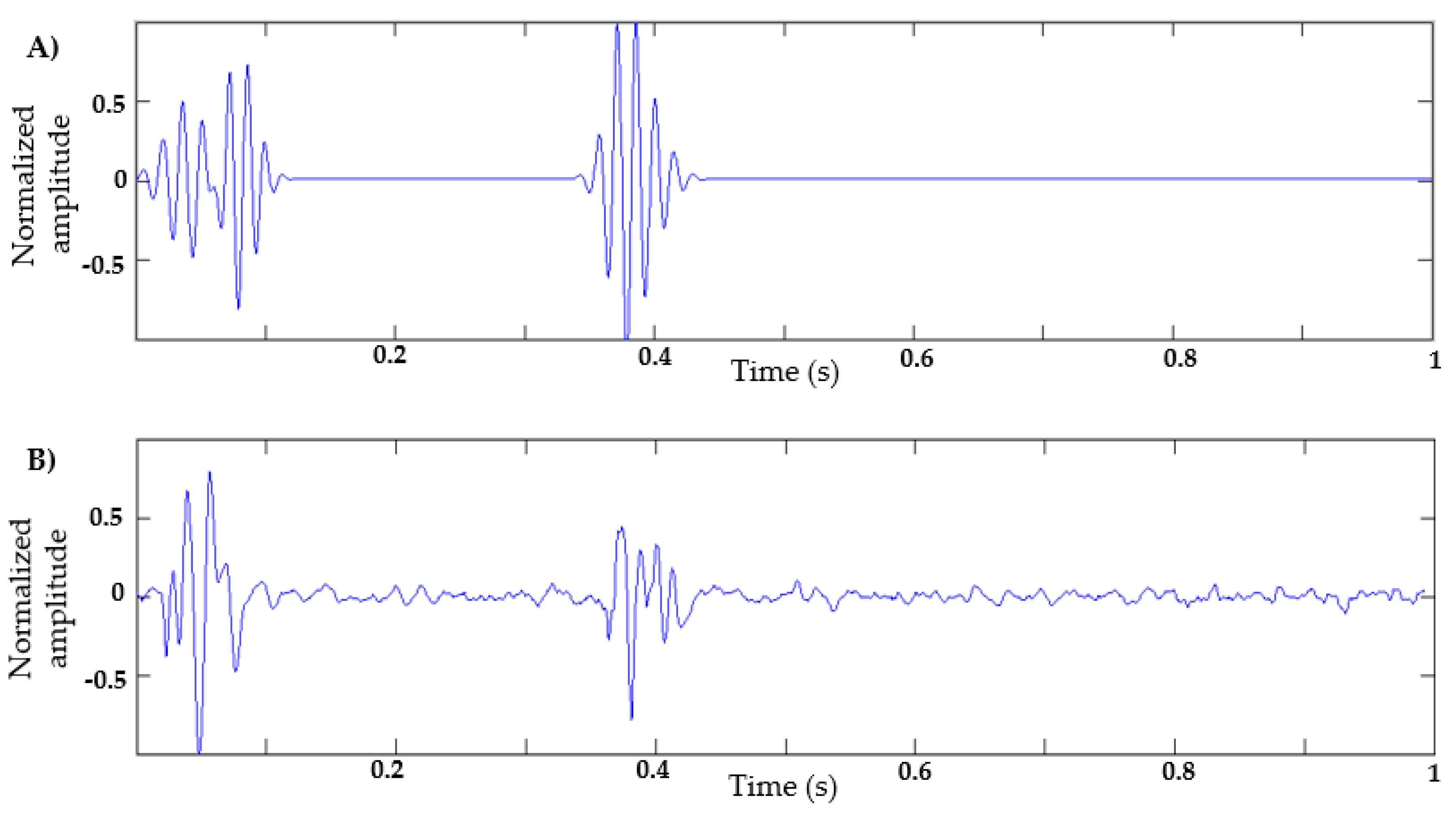
The ordinary differential equation $\dot{z}$ was solved using the numerical Runge–Kutta method of fourth order, using the Matlab software. Using the values in Table 3, we obtain the graph in Figure 9A, which represents the S1 and S2 sounds of a cardiac cycle. Figure 9B shows a natural signal of heart sound.

4.1. Results Using Mel–Cepstral Distortion (MCD)

Mel–cepstral distortion (MCD) is a metric widely used to objectively evaluate audio quality [46], and its calculation is based on Mel-frequency cepstral coefficients (MFCC). This method has been widely used in the evaluation of voice signals, since many automatic voice recognition models use feature vectors based on MFCC coefficients [46]. The parameters used for MFCC extraction are the following: the length of the analysis window (frame) in seconds is 0.03 s, the step between successive windows in second is 0.015 s, the number of cepstra to return in each windows (frame) is 14, the number of filters in the filterbank is 22, the FFT size is 4000, the lowest band edge of mel filters is 0, the highest band edge of mel filters is 0.5, and no window function is applied to the analysis window of each frame.

Basically, MCD is a measure of the difference between two MFCC sequences. In Vasilijevic and Petrinovic [47], different ways of calculating this distortion are presented. In Equation (3), the formula used in [46] is defined, where $C_{MFCC}$ and $\widehat{C_{MFCC}}$ are the MFCC vectors of a frame of the original and study signal, respectively, and L represents the number of coefficients in that frame. $MC{D}_{FRAME}$ represents the MCD result obtained in a frame.

$$MC{D}_{FRAME}={\displaystyle \sum }_{l=1}^L{\left(C_{MFCC}\left[l\right]-\widehat{C_{MFCC}}\left[l\right]\right)}^2$$

(3)

In this work, it was decided to use this objective measurement method to evaluate the similarity between natural and synthetic heart signals, taking into account that heart sounds are audio signals that are typically evaluated using human hearing, and the MFCC coefficients have already been used in the analysis of heart sound signals [9,10,11,12].

A set of 400 natural normal heart sounds taken from the Physionet [30] and Pascal [31] databases were used. Each signal was cut to a single cardiac cycle, with a normalized duration of 1 s, applying a resampling on the signal. Signals were also normalized in amplitude, and those signals with a similar heart rate were chosen. Those natural signals are compared to a total of 50 synthetic heart sounds generated using the proposed method, and 50 synthetic signals were generated using the model [21]. In the case of the model [21], the ${\alpha }_i$ parameters were obtained with random variables in the range of 0.3 to 0.7, in order to generate different wave signals. The other parameters were established as shown in Table 3. Additionally, the synthetic signal was mixed with a white Gaussian noise, as indicated in the article [21]. These synthetic signals have a sampling rate of 2 KHz, a duration of 1 s, and are amplitude-normalized. All signals (natural and synthetic) have a similar heart rate—that is, the size of the systolic and diastolic interval is similar in all the signals.

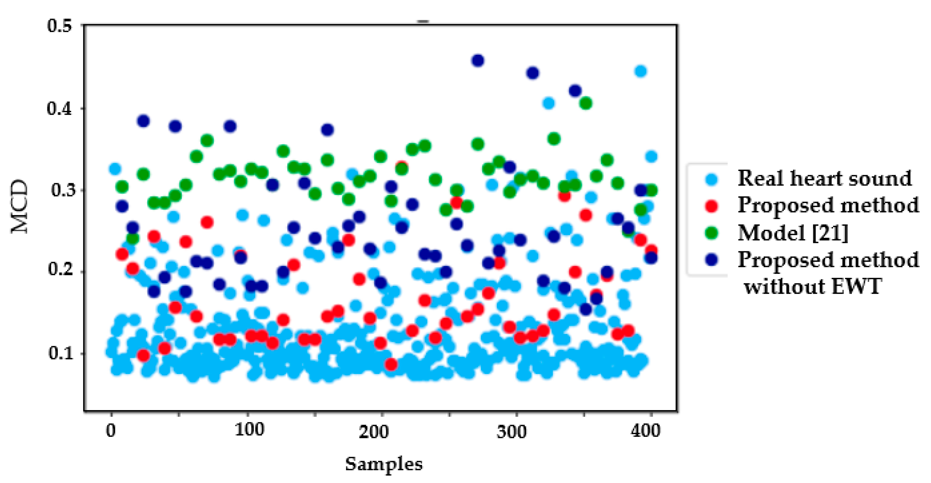
The first evaluation step was to calculate the MCD between the natural signals—that is, the MCD between each natural signal and the remaining natural samples. A total of 399 MCD values were computed and then averaged. This same procedure was applied with the synthetic signals, i.e., computing the MCD between each synthetic signal and each natural signal, obtaining 400 MCD values that were then averaged. Figure 10 shows a schematic of the procedure to compute the MCD. Figure 11 shows the results of the average MCD between the natural signals (blue color), the average distortions of the synthetic signals generated with the proposed method (red color), the average distortions of the synthetic signals generated with the proposed method without applying an EWT algorithm (dark blue color), and the average distortion of the synthetic signals generated with the model in [21] (green color) using the MCD method.

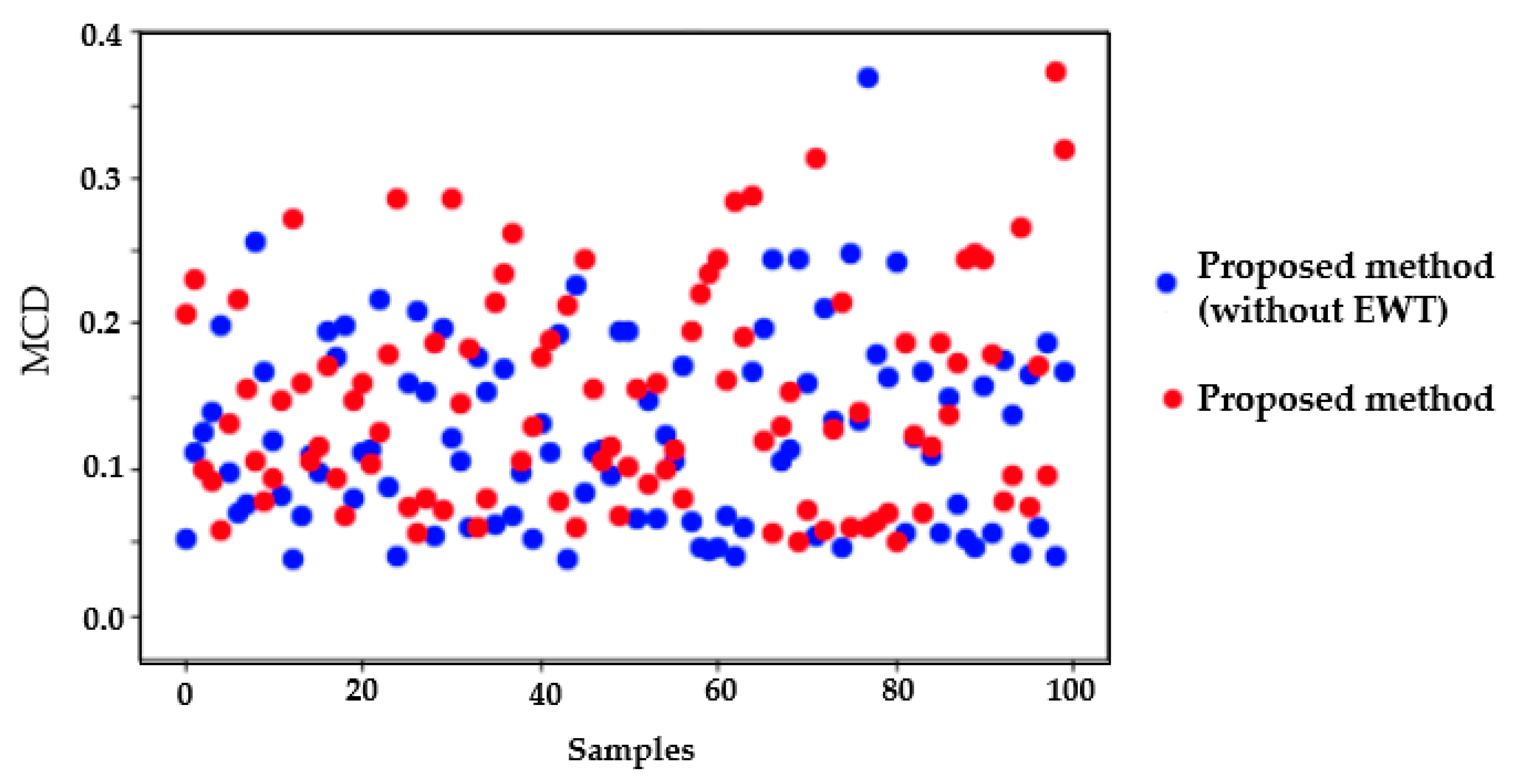
To verify that the generator in the GAN model was not just copying some of the training examples, we computed the MCD distortion of a synthetic signal against each of the signals used in the training dataset. Figure 12 shows the resulting MCD values, with and without the EWT postprocessing. It can be seen that in none of the cases is there an MCD value equal to approaching zero; therefore, the generated signal is not a copy of any of the training inputs.

It can be seen in Figure 11 that the distortions of the natural signals and the signals generated using the proposed method are in the same range, unlike the distortion obtained with the signals generated using the model [21].

4.2. Results Using Classification Models

In this section, different heart sound classification models published in the state of the art are tested [9,10,11,12]. These models focus on discrimination between normal and abnormal heart sounds. They were trained with a total of 805 heart sounds (415 normal and 390 abnormal), obtained from the following databases: the PhysioNet/Computing in Cardiology Challenge 2016 [30], Pascal challenge database [31], Database of the University of Michigan [48], Database of the University of Washington [49], Thinklabs database (digital stethoscope) [50], and 3M database (digital stethoscope) [51].

Table 4. Features extracted in models [9,10,11,12].

Reference	Features
[9]	Six power values (three in systole and three in diastole)
[10]	Nineteen mel–frequency cepstral coefficients (MFCCs) and 24 discrete wavelet transform features
[11]	Statistical domain: mean value, median value, standard deviation, mean absolute deviation, quartile 25, quartile 75, inter-quartile range (IQR), skewness, kurtosis, and coefficient of variation. Frequency domain: entropy, dominant frequency value, dominant frequency magnitude, and dominant frequency ratio. Perceptual domain: 13 MFCCs.
[12]	Six linear prediction coefficient (LPCs) + 14 MFCCs per segment (S1, S2, systole, and diastole)

presents the different characteristics extracted in the proposed classification methods [9,10,11,12]. These characteristics belong to the domains of time, frequency, time–frequency, and perception.

Each feature set was used as input to the following machine learning (ML) models: support vector machine (SVM), k-nearest neighbors (KNNs), random forest (RF), and multilayer perceptron (MLP). In

Table 5. Accuracy results of the methods proposed in [9,10,11,12], taken from article [9].

Feature Extraction	Classifier
	SVM	KNN	RF	MLP
EWT + power [9]	92.42%	99.25%	99.00%	98.63%
MFCC + DWT [10]	90.68%	91.18%	91.42%	91.55%
Statistical, frequency, and perceptual [11]	84.47%	93.66%	93.66%	92.54%
LPC + MFCC [12]	96.27%	95.52%	95.27%	97.26%

, the accuracy results of each one of the combinations of characteristics with the ML models are presented, applying a 10-fold cross-validation. The analysis of these results is described in more detail in [9].

In this work, these classification models were used to test the synthetic signals generated with the proposed method (GAN). Therefore, 50 synthetic signals were used as the test dataset, and the accuracy results are presented in

Table 6. Accuracy results of synthetic signals, using the trained models proposed in articles [9,10,11,12].

Feature Extraction	Classifier
	SVM	KNN	RF	MLP
EWT + power [9]	100%	100%	100%	100%
MFCC + DWT [10]	80%	90%	78%	82%
Statistical, frequency, and perceptual [11]	98%	78%	78%	60%
LPC + MFCC [12]	98%	96%	96%	82%

. The same procedure was done with the synthetic signals without applying the EWT algorithm, with the accuracy results presented in

Table 7. Accuracy results of synthetic signals without applying an EWT algorithm, using the trained models proposed in articles [9,10,11,12].

Feature Extraction	Classifier
	SVM	KNN	RF	MLP
EWT + power [9]	100%	100%	100%	100%
MFCC + DWT [10]	85%	88%	80%	90%
Statistical, frequency, and perceptual [11]	90%	78%	75%	60%
LPC + MFCC [12]	95%	90%	90%	78%

.

The best results were obtained with the power characteristics proposed in [9]. However, in several combinations of characteristics and ML models, precision results greater than 90% were obtained, as was the case of the combination of LPC and MFCC proposed in [12]. From these results, it can be argued that the synthetic signals generated with the proposed method have similar characteristics to the natural signals, since the classification results on both type of signals are similar.

5. Conclusions and Future Work

A GAN-based architecture was implemented to generate synthetic heart sounds, which can be used to train/test classification models. The proposed GAN model is accompanied by a denoising stage using the empirical wavelet transform, which allows us to decrease the number of training epochs and therefore the total computational cost, obtaining a synthetic cardiac signal with a low noise level.

The proposed method was compared with a mathematical model proposed in the state of the art [21]. Two evaluation tests were carried out: the first was to measure the distortion between the natural and synthetic cardiac signals, in order to objectively evaluate the similarity between them. In this case, the mel–cepstral distortion (MCD) method was used, being widely used in the evaluation of audio quality. In this test, the synthetic signal generated with the proposed method obtained a better similarity result with the natural signals compared to the mathematical model proposed in [21].

The second method consisted of using different, pre-trained classification machine learning models with good precision performance, in order to use the synthetic signals as test dataset and verify if the different ML models perform well. In this test, the power characteristics proposed in [9] with the different machine learning models registered the best results. Generally speaking, most of the combinations of features with classification models performed well in discriminating synthetic heart sounds as normal, as shown in Table 4.

According to the results obtained using the MCD distortion metric, and the performance of different ML models, a strong indication can be seen that synthetic signals can be used to improve the performance of heart sound classification models, since the number of samples in the training could be increased.

As future work, we are implementing a GAN-based model that can generate abnormal types of heart sounds, delving into the generation of heart murmurs, since it is very difficult to acquire many samples of a specific type of abnormality. By creating a database of normal synthetic heart sounds and types of abnormalities, we hope to improve the performance of classification systems and advance the detection of types of heart abnormalities, generating significant support for healthcare professionals.