Parallel Broadband Femtosecond Reflection Spectroscopy at a Soft X-Ray Free-Electron Laser

Featured Application

Exploiting the full flux and temporalresolution of SASE-FELs for highly sensitive X-ray absorption measurements.

Abstract

X-ray absorption spectroscopy (XAS) and the directly linked X-ray reflectivity near absorption edges yield a wealth of specific information on the electronic structure around the resonantly addressed element. Observing the dynamic response of complex materials to optical excitations in pump–probe experiments requires high sensitivity to small changes in the spectra which in turn necessitates the brilliance of free electron laser (FEL) pulses. However, due to the fluctuating spectral content of pulses generated by self-amplified spontaneous emission (SASE), FEL experiments often struggle to reach the full sensitivity and time-resolution that FELs can in principle enable. Here, we implement a setup which solves two common challenges in this type of spectroscopy using FELs: First, we achieve a high spectral resolution by using a spectrometer downstream of the sample instead of a monochromator upstream of the sample. Thus, the full FEL bandwidth contributes to the measurement at the same time, and the FEL pulse duration is not elongated by a monochromator. Second, the FEL beam is divided into identical copies by a transmission grating beam splitter so that two spectra from separate spots on the sample (or from the sample and known reference) can be recorded in-parallel with the same spectrometer, enabling a spectrally resolved intensity normalization of pulse fluctuations in pump–probe scenarios. We analyze the capabilities of this setup around the oxygen K- and nickel L-edges recorded with third harmonic radiation of the free electron laser in Hamburg (FLASH), demonstrating the capability for pump–probe measurements with sensitivity to reflectivity changes on the per mill level.

1. Introduction

X-ray absorption spectroscopy (XAS) is a common method for characterizing materials in a variety of fields due to its fundamental simplicity, flexibility and element-specificity. Tuning to absorption edges allows probing the unoccupied electronic states localized around specific elements. Although experimentally more challenging, this information content is especially high at the absorption edges in the soft X-ray regime [1], since core hole lifetimes are longer and spectral features sharper than at higher photon energies. In a pump–probe experiment with sufficiently short pulses, e.g., in free electron lasers (FELs), transient XAS can be used to track changes of the electronic structure during chemical reactions and phase transitions on the femtosecond (fs) to picosecond (ps) scale [2,3,4].

XAS measures the spectral absorption coefficient, i.e., the imaginary part of the index of refraction. Measurements in specular reflectivity additionally measure the real part of the refractive index, which is rigorously connected with the imaginary part, through the Kramers–Kronig transform [5]. Thus, the same spectroscopic information is transported [6]. The most straightforward method of measuring XAS is in transmission by monitoring the intensity of an incident and the transmitted monochromatic beam as a function of photon energy. However, short absorption lengths in the soft X-ray regime necessitate sub-µm thin samples, which can be a prohibitive limitation in terms of properties and manufacturability of the sample. Therefore, XAS is often performed indirectly, by observing either electron yield or drain current resulting from the photoelectric effect or the fluorescence yield. Each of these methods has advantages and disadvantages. Broadly speaking, electron-based methods constitute a powerful approach but limit the obtained information to the surface region and suffer from space-charge and capacitance effects when implemented with intense pulsed sources. Fluorescence based methods are free of such charge effects but struggle from low signal levels in the soft X-ray regime, as the Auger process is dominant and suppresses radiative decay. Furthermore, additional selection rules constraining fluorescent decay as well as competing fluorescence channels can lead to deviations in the spectra that can only be fully interpreted and disentangled [7,8,9] after spectral analysis of the isotropically emitted fluorescence from the sample, using a spectrometer. As in the soft X-ray regime, spectrometers operate with gratings at grazing incidence angles, such spectrometers exhibit small solid acceptance angles, strongly reducing the overall detected signal. Therefore, although a multitude of these methods are applied with great success at synchrotron sources, performing XAS studies at FEL facilities [2,10,11] remains challenging. Another challenge particular to FELs, is the stochastic nature of radiation from the self-amplified spontaneous emission (SASE) process on which most FELs rely (except those that implement seeding). The X-ray pulses produced by the SASE process exhibit a number of Fourier-limited modes of random intensity, which are randomly distributed within overall pulse durations typically on the order of 50 fs and a spectral bandwidth of typically 0.5–1% [12]. Using a monochromator to gain higher spectral resolution enhances the strong intensity fluctuations of the resulting beam and discards a significant part of the incoming flux. For XAS measurements, this means that the incident flux cannot be approximated as constant, but must be measured with the same fidelity, sensitivity and dynamic range as the signal. Furthermore, monochromators can significantly elongate the FEL pulse duration due to grating induced pulse-front tilting, which scales with the number of illuminated grating lines and is thus especially severe (up to a picosecond) at very high spectral resolutions.

Here, we demonstrate the use of a transmission grating beam-splitter to split the FEL into practically identical signal and reference beams, both of which are analyzed in-parallel with the same spectrometer after interaction with the sample. Thus, both FEL fluctuations, as well as possible nonlinearities in the detector are exactly reproduced in both signals and can thus be renormalized.

Unlike comparable schemes with monochromatic beams [13,14,15,16], our method places the grating for spectral analysis after the sample interaction, so that the full SASE bandwidth contributes to the measurement. For a given FEL fluence on the sample, measuring the collimated specular reflection as opposed to isotropic fluorescence provides much stronger signals. The signal intensity can even be tuned by adjusting the angle of incidence to optimally exploit the detector dynamic range, since varying the angle will generally alter the spectral shape but not change the spectroscopic information. Here, we analyze the sensitivity of this experimental scheme for spectral (e.g., pump-induced) changes by evaluating pairs of simultaneously recorded reflectivity spectra of NiO at the oxygen K- and nickel L_2,3-edges, respectively.

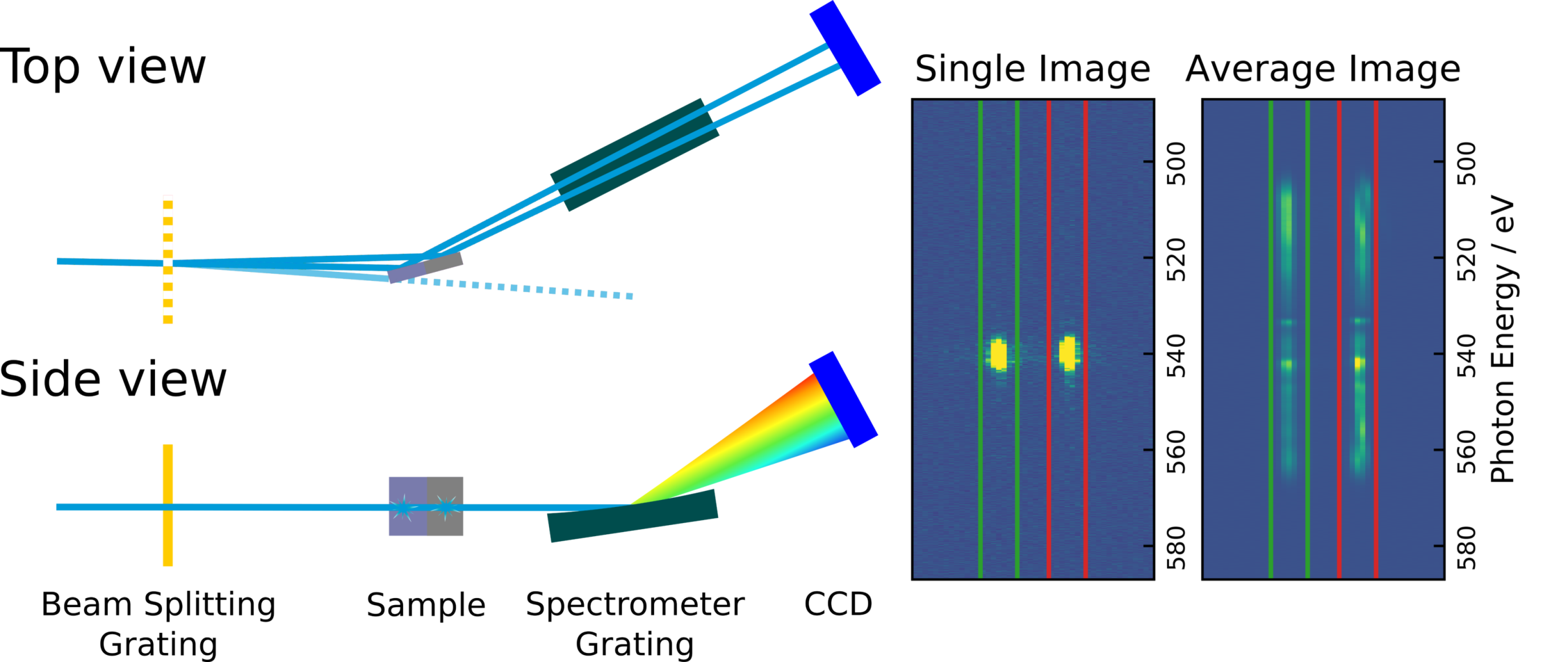
2. Experimental Design

A simplified schematic of the setup is shown in Figure 1. Measurements were performed with the MUSIX experimental end station [17] at the FL24 beam line of the free-electron laser in Hamburg (FLASH). The FEL was tuned to generate third harmonic radiation around the oxygen K- and nickel L_2,3-edges (from 506 eV to 566 eV and 842 eV to 887 eV, respectively), producing bursts of 40 pulses with 10 µs spacing within the burst and 10 bursts per second. Before the beam line, the beam is defined by two apertures: 5 mm apertures are used at the O K-edge and 2 mm apertures at the Ni L-edges. Then, the average FEL pulse energy was monitored using the signal from an X-ray gas monitor detector (XGMD) [18], after which the fundamental radiation was suppressed by a 13 meter long gas attenuator unit containing 9.7 × 10⁻² mbar of neon (O K-edge) or 1.7 × 10⁻² mbar of krypton (Ni L-edges) in addition to two Si membrane filters of 401 nm and 200 nm thickness.

The beam is then split horizontally by a transmission grating of 3.8 mm height and 0.9 mm width, optimized to produce similar intensity in the zeroth and first diffraction orders: It is made from a Si-membrane of 1.1 µm thickness with rectangular grooves of 960 nm depth and 7.9 µm period at 50% aspect ratio. The zeroth and first diffraction orders are each directed onto the sample, focused by bendable mirrors to a spot of about 35 µm height and 80 µm width, at a grazing angle $\theta$ of 11.5°. The specular reflections of both beams are analyzed by the spectrometer of the MUSIX endstation [17], consisting of a variable line spacing grating and an in-vacuum charge-coupled device (CCD) (GreatEyes Model GE-VAC 2048 2048). The 13.5 µm square pixels of the CCD were read out with an ADC clocked with 3 MHz in high gain mode and 16 pixel binning orthogonal to the spectral axis to increase the frame rate and decrease noise while preserving the spectral resolution. This resulted in a framerate of 5 Hz. The FEL, producing bursts of 10 Hz, was chopped accordingly, so that each detector image represented an average over one burst of 40 pulses. The photon energy dispersion on the CCD was measured as 10.73 pixel/eV at the O K-edge and 7.8 pixel/eV at the Ni L-edges.

Samples consisted of epitaxial NiO films of 40 nm thickness, grown on MgO(001) substrates. A 2 nm thick MgO underlayer was deposited by radio frequency magnetron sputtering in 3 mTorr argon at a temperature below 100 °C followed by a NiO layer that was deposited at 700 °C in an Ar (90%)/O₂ (10%) gas mixture at a pressure of 3 mTorr and was then annealed in-situ at the same temperature (700 °C) for 15 min in the same Ar-O₂ gas mixture.

To acquire spectra within a wider window than the 0.5–1% natural bandwidth of the FEL, the photon energy is scanned in steps of 0.75 eV by varying the undulator gap. As datasets include multiple scans over the desired range, data taken at the same undulator settings are averaged in the data analysis. Two spectra are extracted from each image by integration along the non-dispersive direction of the CCD within manually selected regions of interest such as indicated in Figure 1. Before computing the average spectrum, each single-image spectrum was cropped to the range deviating less than 1 % from the FEL photon energy set-point, as no significant intensity is found outside this window.

3. Results and Discussion

To understand the benefits of acquiring two spectra in-parallel, we consider the measured spectral intensity on the detector $S\left(\omega \right)$, which depends on the photon frequency $\omega$ for each beam, to be proportional to the spectral reflectivity $R\left(\omega \right)$of the sample, the diffraction efficiency $O$of the beam-splitting grating in the zeroth or first order and the spectral intensity $I\left(\omega \right)$ of the FEL:

$$\begin{gathered} S_1\left(\omega \right)\propto R_1\left(\omega \right)O_{1}I\left(\omega \right) \\ {S}_2\left(\omega \right)\propto R_2\left(\omega \right)O_{0}I\left(\omega \right) \end{gathered}$$

(1)

It is apparent that the measured spectrum $S\left(\omega \right)$ of a single beam can be used to measure the reflected spectrum $R\left(\omega \right)$, if the FEL intensity $I\left(\omega \right)$ is either known or constant. If many pulses are averaged, SASE fluctuations average out, but potential slow drifts of the average pulse energy remain. Since the third harmonic radiation intensity scales roughly with the square of the fundamental [17], slow fluctuations are mitigated by normalizing each spectrum with the square intensity measured by the XGMD which monitors the fundamental radiation of the FEL further upstream. This leads to the FEL spectra shown in Figure 2a,b, each pair was measured in-parallel using 10⁵ SASE pulses within four minutes. Synchrotron spectra of reflectivity and drain current recorded on the same sample with a similar angle of incidence ($\theta$ = 11° for the O K-edge, $\theta$= 12° for the Ni L_2,3-edges) are shown for comparison and demonstrate a good agreement to the FEL spectra. The FEL-reflectivity spectra recorded at these angles reproduce the relevant structures of the drain current absorption spectra. We ascribe the minor differences to sample inhomogeneity and the difference of the incident angle. Especially the O K-edge spectra also show signs of surface contamination with water (especially the structure above 545 eV), as the sample was exposed to air both before and between FEL and synchrotron measurements. In the following, we analyze how accurate changes in one spectrum due to FEL fluctuations can be used to measure the changes in the other spectrum. Our main motivation for recording two spectra in-parallel is to exploit one of them as a spectrally resolved intensity reference in a pump–probe scenario. In this case, a crucial parameter is the precision with which (pump-induced) changes in one spectrum may be determined from the other. The fraction of fluctuation that cannot be explained from the variations in the reference spectrum is quantified by the so-called fraction of variance unexplained (FVU). The FVU for a set of $N$ pairs of spectra equal unity minus the coefficient of determination $r^2$ between both spectra, which is in this case, the square of the Pearson correlation coefficient$r$:

$$r\left(\omega \right)=\frac{{{\displaystyle \sum }}_{i=1}^N\left(S_1^i\left(\omega \right)-{\overline{S}}_1\left(\omega \right)\right)\left(S_2^i\left(\omega \right)-{\overline{S}}_2\left(\omega \right)\right)}{\sqrt{{{\displaystyle \sum }}_{i=1}^N{\left(S_1^i\left(\omega \right)-\overline{S_1}\left(\omega \right)\right)}^2}\sqrt{{{\displaystyle \sum }}_{i=1}^N{\left(S_2^i\left(\omega \right)-\overline{S_2}\left(\omega \right)\right)}^2}}$$

(2)

$$FVU=1-r^2$$

(3)

Here, $\overline{S}$ denotes the average spectrum over the set. We find that minor alignment imperfections and pointing drifts can lead to a small offset along the dispersive direction of the detector between two simultaneously recorded spectra. Similar to previous work [15], this offset is determined by shifting the reference spectrum along the dispersive axis (see Appendix A for details) such that the logarithmic FVU, integrated over the entire spectrum, is minimized. The offset is determined in this way for every measurement (each in the order of several minutes) separately, yielding a shift between one and three pixels, i.e., some tens of µm on the CCD detector. The optimized spectrally resolved FVU is shown in Figure 2 and reproduces the structure of the spectrum as it scales inversely with the reflected intensity. The scaling of the FVU with intensity is shown in Figure 3a and is compared to a simulation of the FVU which may be expected from of a Poisson-distributed noise process, scaling with the square root of the intensity like a photon shot noise (orange), and an additional normally-distributed noise process with constant variance like readout noise (green). Since the fast readout of the CCD prevented a calibration of the sensitivity from single-photon incidences, the number of photons per detector count was estimated based on the assumption that the noise level at high intensities is dominated by photon shot noise, as was found in a similar setup before [15]. This assumption is supported by the scaling behavior shown in Figure 3a and is in rough agreement with the manufacturer specifications of the CCD.

Figure 3b further illustrates the uncertainty with which the ratio between the reflectivity probed by both beams may be determined with increasing acquisition time. This uncertainty is the precision with which pump–probe changes in one spectrum could be detected. To this purpose, the undulators are tuned to the Ni L₃-edge. Without scanning the undulators, the ratio between the intensities in both spectra was evaluated. Two exemplary regions in the spectra were analyzed: First, a 245 meV region around the L₃-edge peak at 857 eV (corresponding to two rows on the detector). Second, an equally sized window from the same dataset was evaluated 1 eV above the peak, where the detected intensity was lower by about a factor of nine on average, due to both the lower reflectivity and the FEL being tuned to the L₃-edge. The plot shows the relative uncertainty with which the ratio may be determined for increasingly larger subsets of CCD images, randomly drawn (without replacing) from an 80-min measurement. Two different measures for the uncertainty are shown: First, the uncertainty regarding the parallel acquisition, which considers that the correlation between the two intensities reduces the uncertainty for the estimator of the mean. This error propagation was discussed previously [15] and is reiterated in Appendix B. Second, the error is calculated under the assumption that the fluctuations of both intensities are uncorrelated, which would be the case if the spectra had been recorded consecutively instead of in-parallel.

4. Conclusions

As demonstrated in Figure 3b, the acquisition of two spectra in-parallel merits about one order of magnitude of sensitivity compared to consecutive acquisition. Spectral changes can be monitored within the entire FEL bandwidth at the same time. The sensitivity in the middle of the FEL spectrum reaches a 10⁻³ relative reflectivity change within about 10 min of acquisition for a 245 meV window. The reflectivity spectra acquired in this way reproduce the features of conventional X-ray absorption spectra, so that equivalent information may be gained by pump–probe experiments in reflectivity. As the spectrometer grating analyzes the full reflected beams after sample interaction, the temporal resolution is not diminished by monochromatization. This makes the presented setup ideally suited for time resolved XAS and reflectivity studies in FELs.