Article

Application of Satellite Remote Sensing in Monitoring Elevated Internal Temperatures of Landfills

1
Department of Civil, Construction and Environmental Engineering, University of Alabama at Birmingham, Birmingham, AL 35294, USA
2
Department of Environmental Health Science, University of Alabama at Birmingham, Birmingham, AL 35294, USA
3
Department of Electrical and Computer Engineering, Rowan University, Glassboro, NJ 08028, USA
4
Department of Mechanical Engineering, Rowan University, Glassboro, NJ 08028, USA
5
Department of Civil and Environmental Engineering, Rowan University, Glassboro, NJ 08028, USA
*
Author to whom correspondence should be addressed.
Appl. Sci. 2020, 10(19), 6801; https://doi.org/10.3390/app10196801
Submission received: 30 July 2020 / Revised: 8 September 2020 / Accepted: 8 September 2020 / Published: 28 September 2020
(This article belongs to the Special Issue Hazardous Waste Treatment)

Abstract

:
Subsurface fires and smoldering events at landfills can present serious health hazards and threats to the environment. These fires are much more costly and difficult to extinguish than open fires at the landfill surface. The initiation of a subsurface fire may go unnoticed for a long period of time and undetected fires may spread over a large area. Unfortunately, not all landfill operators keep or publish heat elevation data and many landfills are not equipped with a landfill gas extraction system to control subsurface temperatures generated from the chemical reactions within. The timely and cost-effective identification of subsurface fires is an important and pressing issue. In this work, we describe a method for using satellite thermal infrared imagery at a moderate spatial resolution to identify the locations of subsurface fires and monitor their migration within landfills. The focus of this study was the Bridgeton Sanitary Landfill in Bridgeton, MO, USA where a subsurface fire was first identified in 2010 and continues to burn today. Observations from Landsat satellites over the last seventeen years were examined for surface temperature anomalies (or hot spots) that may be associated with subsurface fires. The results showed that the locations of hot spots identified in satellite imagery match the known locations of the subsurface fires. Changes in the hot-spot locations with time, as determined by in situ measurements, correspond to the spreading routes of the subsurface fires. These results indicate that the proposed approach based on satellite observations can be used as a tool for the identification of landfill subsurface fires by landfill owners/operators to monitor landfills and minimize the expenses associated with extinguishing landfill fires.

1. Introduction

Currently, there is no reliable and cost-effective method available in the United States (U.S.) for detecting and monitoring subsurface smoldering events (SSEs) and related thermal imbalances at U.S. landfills [1]. Such a method is needed as a timely warning tool for the identification of the location and spatiotemporal extent of subsurface “hotspots,” while also aiding in the prevention or minimization of costly subsurface fires and thermal damage to liners and gas/leachate handling systems. The space borne remote sensing of landfill surface temperatures by thermal infrared sensing offers a promising approach. As discussed below, interpretation of the publicly available Landsat data archive enables the monitoring of large areas, such as landfills. The nondestructive, noninvasive methods described in this paper allow for the observation of multiple locations quickly and at low-to-no cost and the assembly of a satellite image archive that indicates changes in the thermal state of landfill surfaces over time. Further algorithmic interpretations of these thermal–areal time series can be used to isolate persistent hotspot signatures by filtering externally forced thermal variations (e.g., from seasonal thermal trends) and short-term thermal excursions [2]. Moreover, with further development, the algorithms presented herein can serve as a basis for an automated monitoring/warning method. For example, the application of machine learning to sudden-change detection could ultimately reduce the burden associated with human-in-the-loop monitoring and facilitate expert event verification and the pursuit of remedial action. Using this algorithmic approach, we present our case study and the obtained preliminary simple stationary statistical metrics (e.g., mean and standard deviation) for the data collected during the study period, with the results indicating that accumulated subsurface heat can be detected by satellite images. We identified the 2010 onset and migration of an SSE in the Bridgeton Sanitary Landfill, with the remote sensing results comparing favorably to ground observations during the same time period.
Previously researchers have examined four landfills located in North America (Michigan, New Mexico, Alaska, and British Columbia) to investigate the thermal states of municipal solid waste (MSW) landfills as a function of usual operational conditions and climatic regions [3]. A comprehensive study has also been conducted to assess the physical and thermal properties of wastes affecting heat transfer and fire ignition [4,5]. In accordance with many other studies, this work showed that in landfills with no SSE or other long-term thermal anomalies, the usual heat generated in MSW landfills is largely the byproduct of the biological decomposition of organic waste along with leachate and gas [6,7,8,9,10,11,12,13]. Under these conditions, the landfill temperature remains close to the air temperature at shallow depths and near the edges of the landfill and reaches maximum values relative to the air and ground temperatures near the areal center and at intermediate depths. Observations indicated that a baseline “healthy” landfill thermal state can be observed by satellite-based remote sensing [3].
Indeed, this technology has been used previously to map and monitor landfills. For example, Landsat Thematic Mapper (TM) images were used to monitor the Al-Qurain landfill in Kuwait and observed a 1–4 °C temperature elevation for the surface of the landfill site relative to the surrounding desert area [14]. A similar study at the Trail Road landfill site near Ottawa, Canada observed an average 9 °C temperature elevation from 1985 to 2009 [15]. These studies demonstrate that satellite-based remote sensing applications that use time series analysis and appropriate image processing techniques can identify and map landfill sites based on differences between baseline surface temperatures and their surroundings. However, none have focused on the detection and monitoring of the evolution of persistent hotspots as an indicator of landfill health disturbance.
Subsurface heating activities result in higher surface temperatures by the transfer of heat from the interior to the landfill surface [2,16]. Data from landfills experiencing SSEs, “subsurface oxidation events,” or “elevated temperatures” suggest that temperatures inside landfills can reach 100–125 °C and even 150 °C in some cases [17]. In such cases, subsurface heating manifests as a hotspot with a temperature exceeding the normal elevation in baseline temperature. Accordingly, thermal imaging of the landfill surface, inferential heat transfer analysis, and the correction of baseline-temperature elevation can provide a viable and efficient method for hotspot detection, which may enable smolder/fire detection and perhaps prevention. Once the locations, timeline, and extent of an SSE or related event are identified, site operators will be better equipped to determine the appropriate remedial actions to be taken.

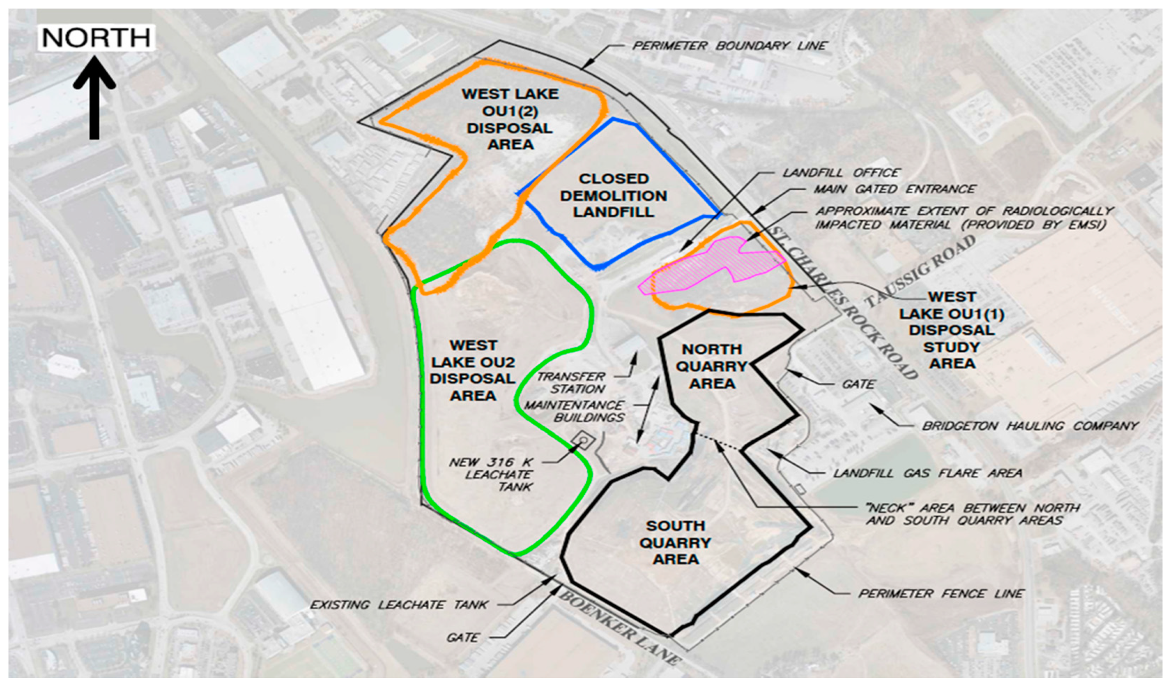
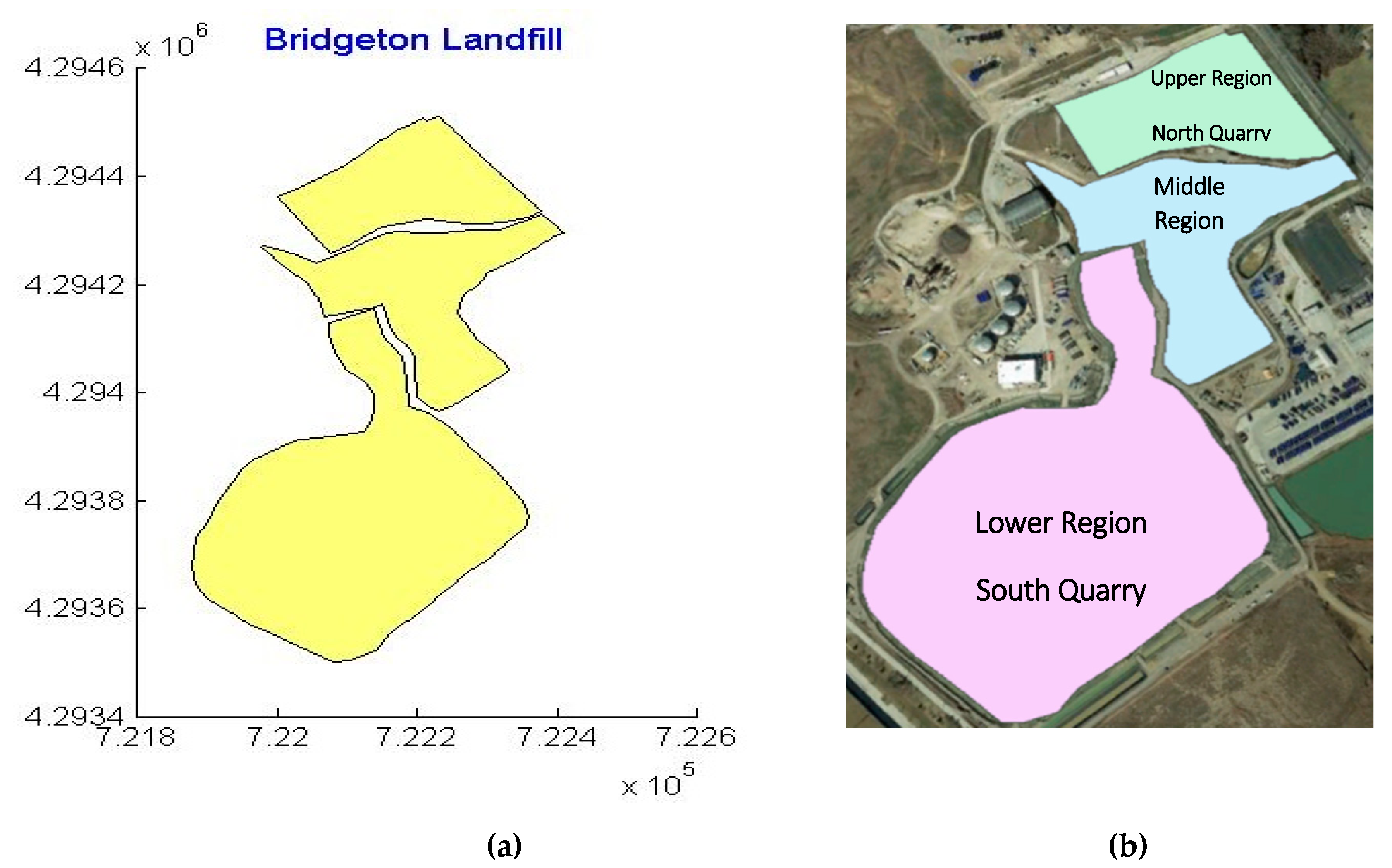
2. Study Goal and Site Description

The goal of this paper is to introduce methodologies for the remote satellite monitoring of the location and movement of subsurface thermal events within landfills, such as smolders and fires. As a case study, these methods were applied to the Bridgeton Sanitary Landfill in Bridgeton, Missouri, U.S., where abnormal subsurface thermal activity has been ongoing since 2010 [18,19]. The Bridgeton Sanitary Landfill in Bridgeton, MO (GPS: 38.767°, −90.443°), roughly 20 miles from downtown St. Louis, MO, is part of a larger site containing five distinct waste areas, a transfer station, and a maintenance building (Figure 1).
This landfill is divided into the North (adjacent to nuclear waste disposal area) and South Quarries, which are connected by a narrow band called the “Neck.” The North (upper) and South (lower) Quarries cover an area of approximately 52 acres. Waste placement at the Bridgeton landfill commenced around 1985 and ceased in December 2004. The total waste thickness at the end of the waste acceptance period was reported to be approximately 320 feet, with 80 feet of waste above the ground surface [21]. The landfill accepted approximately 17,000,000 in-place cubic yards of waste, including commercial, industrial, and municipal solid wastes. The Bridgeton landfill has a leachate collection system and is equipped with 200 temperature and gas well monitoring units. In our analysis, measurements from these sources were used as ground truth for comparison with the remote sensing results. In late 2010, a subsurface elevated temperature event was confirmed in the southern half of the landfill. This SSE, also known as a “subsurface fire (SF),” later expanded in all directions. Stark (2013) estimated the expansion rate of underground combustion in the South Quarry area to be 2.8–3.0 feet per day. This expansion rate estimate was later adjusted to 1–2 feet per day [21,22]. The smoldering event appears to be contained in the South Quarry [23].

Satellite Data Acquisition and Processing

The U.S. Geological Survey (USGS) Earth Explorer tool provides the ability to query, search, and order satellite images, aerial photographs, and cartographic products from several sources. However, none of these representations contain information related to temperature. To determine land surface temperature (LST) distributions, Level 1 satellite images of the exact location of the Bridgeton Sanitary Landfill (GeoTIFF format) were downloaded from the USGS online archive (https://earthexplorer.usgs.gov) and were then processed as described below. Observations from Landsat satellites were used to detect the thermal state of the Bridgeton landfill area and to identify thermal anomalies at its surface. All relevant Landsat data generated between 2000 and 2016 were downloaded and images with only slight (less than 10%) overall cloud contamination were retained. All retained images were then subjected to an image acceptance test, i.e., an algorithm designed to use the Quality Assessment band (now available with downloaded data for Landsat 5, 7 and 8) to accept only images (in this study, the landfill scene) that have no clouds, snow, water, or other land cover that may lead to misleading results. In addition, the images were visually checked to ensure that the landfill area was not obscured by clouds. Due to cloud contamination of the imagery and because of the long, 16-day revisit time of Landsat satellites, the average annual number of clear-sky images collected was seven, for a total of 115 images over the 16-year time period. No reliable data were available between December 2011 and March 2013 as the Landsat 5 archive ended in November 2011, Landsat 8 was launched in April 2013, and the Landsat 7 data for 2012 were found to be unusable for this analysis because of sensor problems. The missing 2012 data is unfortunate, but only affect 15 months out of 204. Hotspots can still be tracked for over 93% of the period of interest.
Images from 2000–2011 were obtained using the Landsat 5 TM. Starting from 2013, we acquired data from the Landsat 8 Operational Land Imager (OLI) and Thermal Infrared Sensor (TIRS) instruments. The number and positions of the spectral bands in the Landsat sensors differed, but we used all sensors that provided observations in the visible, near-infrared (near-IR), and thermal infrared (TIR) bands. The spatial resolution of all the sensors in the visible and near-IR bands was 30 m, and that of the TIR band was 120 m on the TM sensor and 100 m on the TIRS sensor. However, the USGS provides observations in these bands resampled to 30-m resolution, which is the same as that of the visible and near-IR bands. All scenes were acquired at Level 1B with observations in all bands provided as 8 bits for the TM and 16 bits for the OLI and TIRS.
Preprocessing of the satellite imagery was performed according to the procedure described in the Landsat handbook [24]. Digital numbers (DNs) in the optical bands were converted first to radiance and then to reflectance. The reflectance values were corrected for variable Sun–Earth distances and normalized to the overhead Sun by dividing the reflectance by the cosine of the solar zenith angle. Observations in the TIR band were converted first to radiance and then to brightness temperature Tb values. The calibration coefficients used to convert DN counts into physical values (reflectance and brightness temperature) were obtained from metafiles supplied by the USGS with the Landsat imagery (Table 1).
To estimate the LST from the observed IR brightness temperature Tb, we used the approach below [25]:
LST = T b 1 + ( λ   T b d ) ln ( e )   ,
where T b is the blackbody temperature; λ is the wavelength of the emitted radiance; d is defined by d = ch/kB, where the velocity of light (c = 3 × 10⁸ m/s) is multiplied by Planck’s constant (h = 6.26 × 10⁻³⁴ J.s) and divided by Boltzmann’s constant (kB = 1.38 × 10⁻²³ J/K); and e is the land surface emissivity. The emissivity is calculated using Equation (2) [26]:
e = 0.004 +   0.986   P V ,
where PV is the proportion of vegetation, which is sometimes referred to as the fractional vegetation cover and calculated using Equation (3):
P V = [ NDVI NDVI min NDVI max NDVI min ] 2 .
In this equation, NDVI is the normalized difference vegetation index. To calculate the NDVI of the surface, we used Equation (4) [27]:
NDVI = [ NIR   RED NIR + RED ] ,
where NIR represents the near-IR band reflectance and RED is the visible red band reflectance. NDVImax and NDVImin in Equation (3) are the maximum and minimum NDVI indices in the image, respectively, for which NDVImax = 0.5 for vegetation and NDVImin = 0.2 for soil can be used [28].
Atmospheric scattering and absorption may also affect the estimation of land surface emissivity from NDVI [29]. In this study, the effects of scattering and absorption on the NDVI—particularly the atmospheric absorption by carbon dioxide and water vapor—were not taken into consideration. This could result in an overall underestimation of the absolute LST by 1–3 K. However, it would not affect the contrasts and gradients of the observed surface temperature because (1) there is no reason to expect meaningful variations in the atmospheric composition over the area of a landfill and (2) such uncertainties relative to the nominal absolute temperatures, which were subsequently considered, were not found to meaningfully impact hot spot detection.

3. Approach

Landsat images were processed using in-house MATLAB code. All images were read with a 1-km buffer around a central point of the landfill. The buffer generated an image with 67 × 67 pixels, which covers approximately 4 km2 for all bands, including the LST thermal images. The advantage of this approach is that the landfill’s surrounding area can be analyzed if needed [30]. For convenience, the resulting image (67 × 67) was masked with an overall landfill shape file, as illustrated in Figure 2. To align our analysis with prior observations of the Bridgeton landfill, we also divided the landfill area into three smaller regions: a lower region (the South Quarry where most of the landfill activities occur), a middle region (the Neck area), and an upper region (the North Quarry and radioactive waste areas), each of which is well defined by its own shape file, as shown in Figure 2.
This approach has several advantages: (a) the effect of any extreme reading due to water or buildings or any other land cover can be isolated to ensure that only readings within the study area are considered; (b) each area/subarea can be analyzed separately, as described in the following; (c) hotspots that move within each area/subarea can be easily traced over time spans of many years; and (d) the status of each landfill subarea can be tracked independently.

4. Results

In this section, several interpretations of the Landsat LST data with respect to the landfill are presented. While these interpretations yield quantitatively different results, the general trends identified by each enable hotspot detection. This unanimity of interpretation suggests that these algorithms are robust with respect to each other and yield similar conclusions regarding the spatial and temporal extents of hotspots determined by others. Here, we use simple stationary statistical metrics (e.g., mean and standard deviation) to demonstrate proof-of-principle use of LST measurements for landfill hotspot detection and monitoring. Future extensions of these approaches, which are described below, may involve more rigorous (thermal) change detection techniques such as cumulative sum control (CUSUM) and related online change-detection algorithms.
LST-change interpretations are presented here at three levels of spatiotemporal resolution. This has the advantage of reducing complexity when detecting or monitoring landfills, i.e., there is no need to expend computational resources or human-in-the-loop attention for the observation of baseline thermal behavior, but upon detection of a hot spot, different degrees of spatial resolution can be invoked. Initially, the landfill is treated as a whole system characterized by average, minimum, and maximum LSTs across the entire spatial domain. Time series trends enable the observation of baseline and excursive behaviors, although with no distinct spatial resolutions. Subsequently, the landfill is divided into regions (determined by both historical definitions as well as automated clustering analysis) to resolve the general location of the enhanced thermal activity. For sites like the Bridgeton landfill that are adjacent to sensitive assets (e.g., the radiologically impacted zone indicated in Figure 1), such determination indicates the areal extent that may require action without adding further complexity (quantity, noise, uncertainty) from pixel-resolved (30 × 30 m) LST measurements. Lastly, we consider pixel resolved LST measurements of the Bridgeton landfill to further demonstrate the robustness of our analysis. As demonstrated below, each of these analyses based on satellite remote sensing was corroborated by independent ground-truth data and field measurements for this well-studied site [21,23,31].

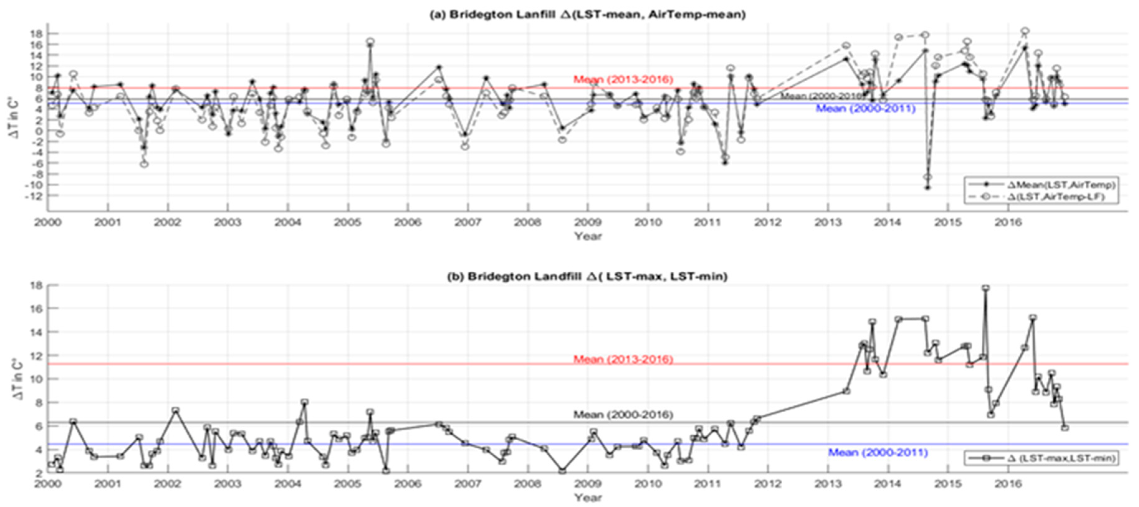
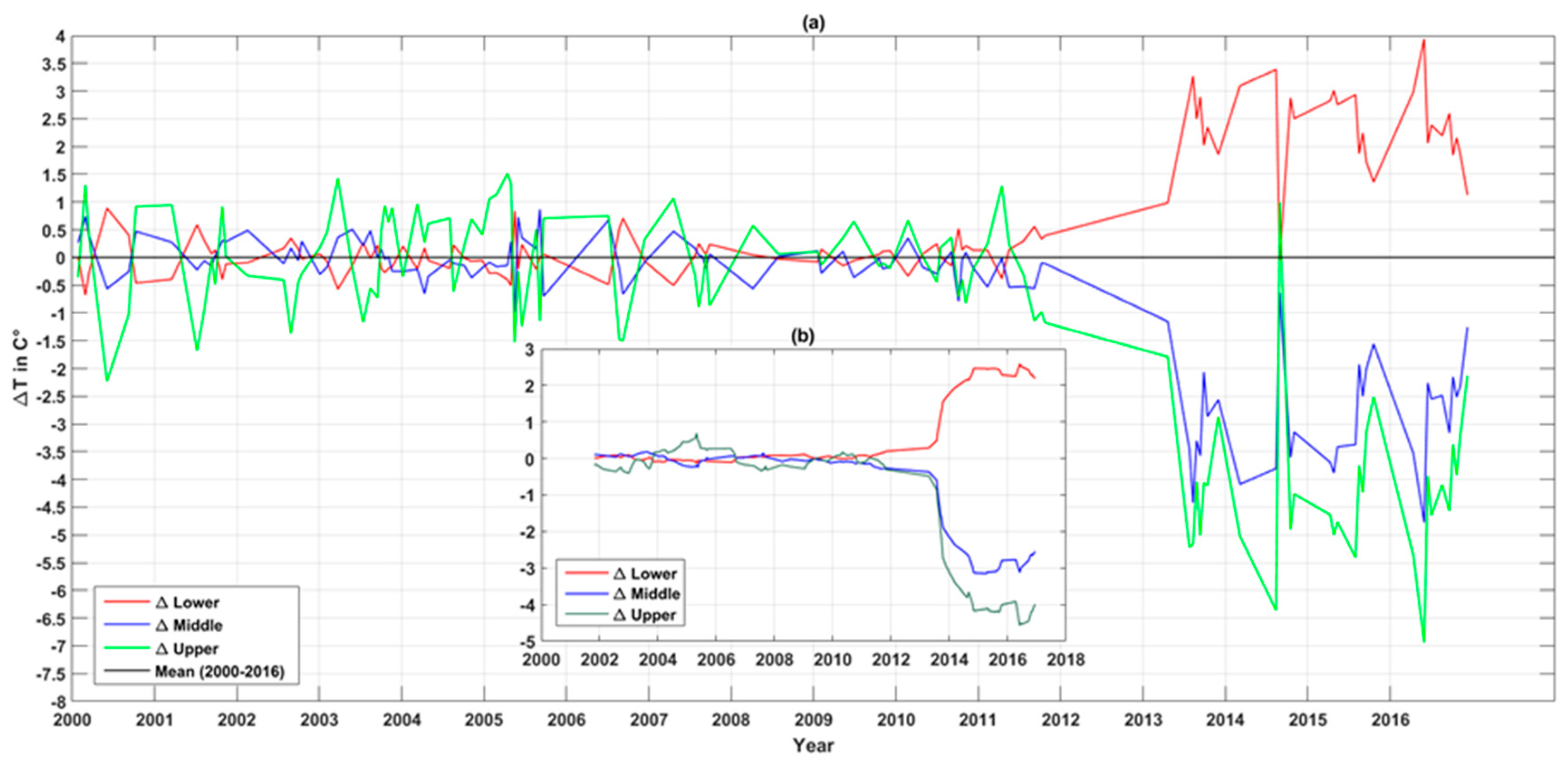
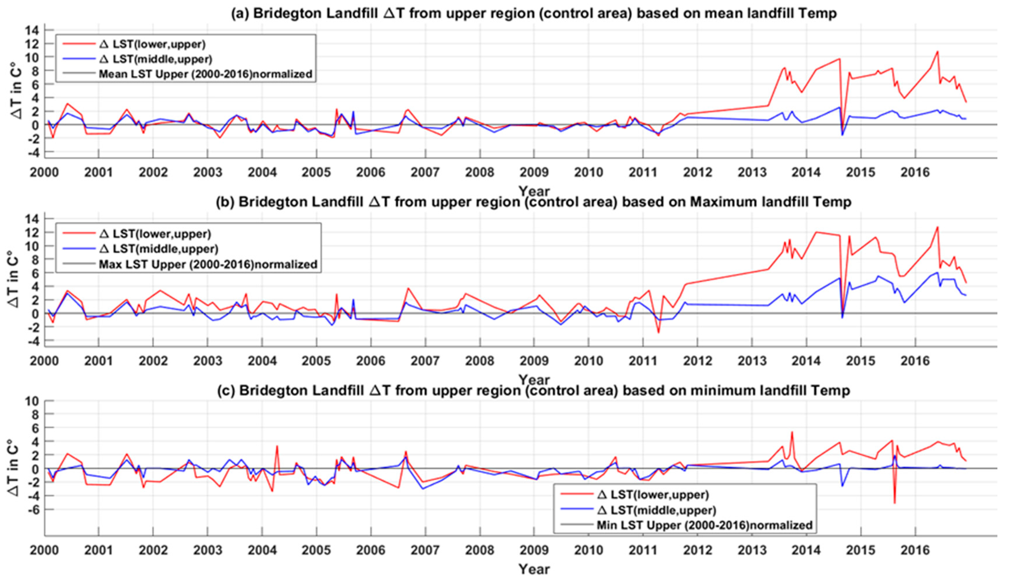
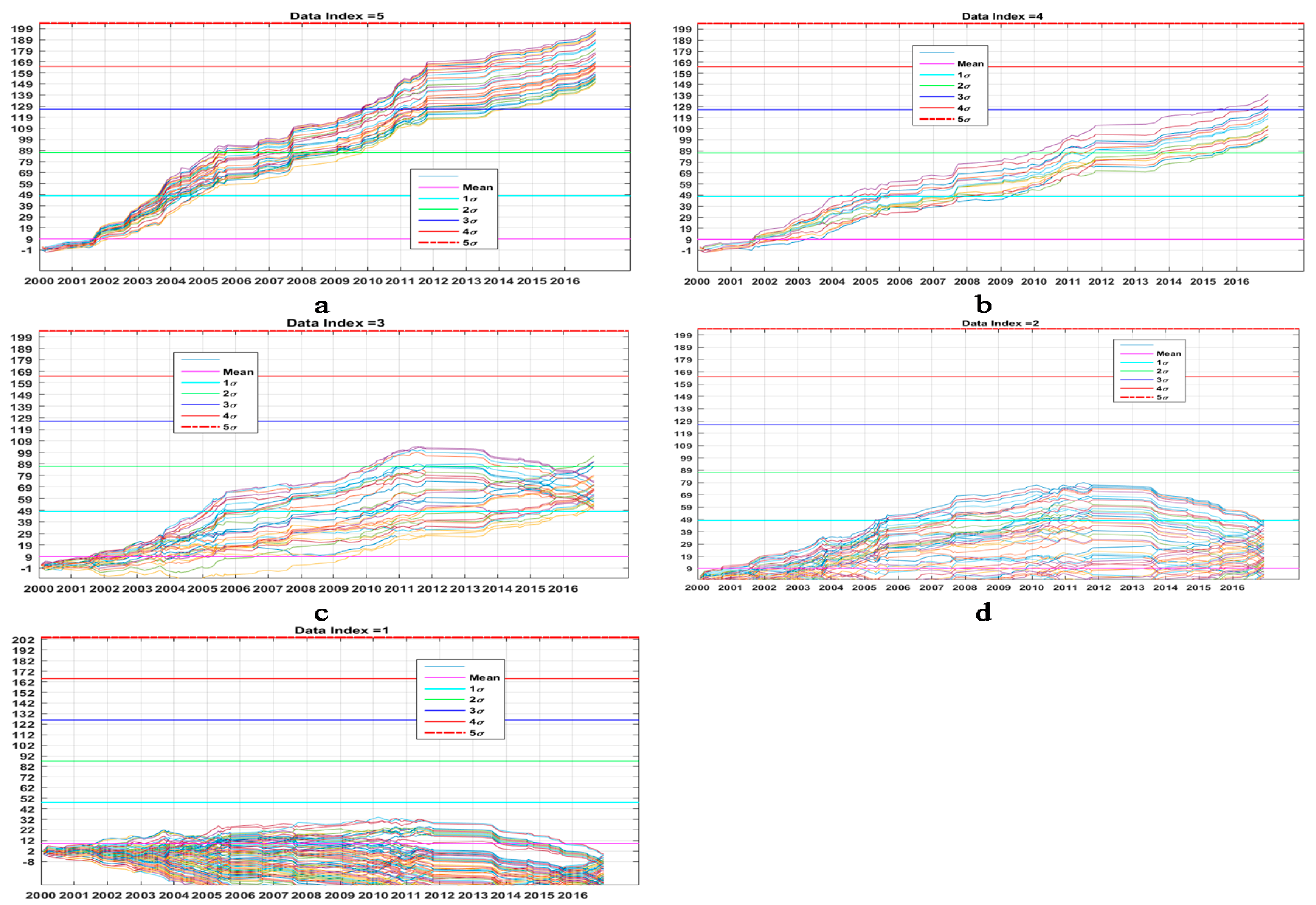
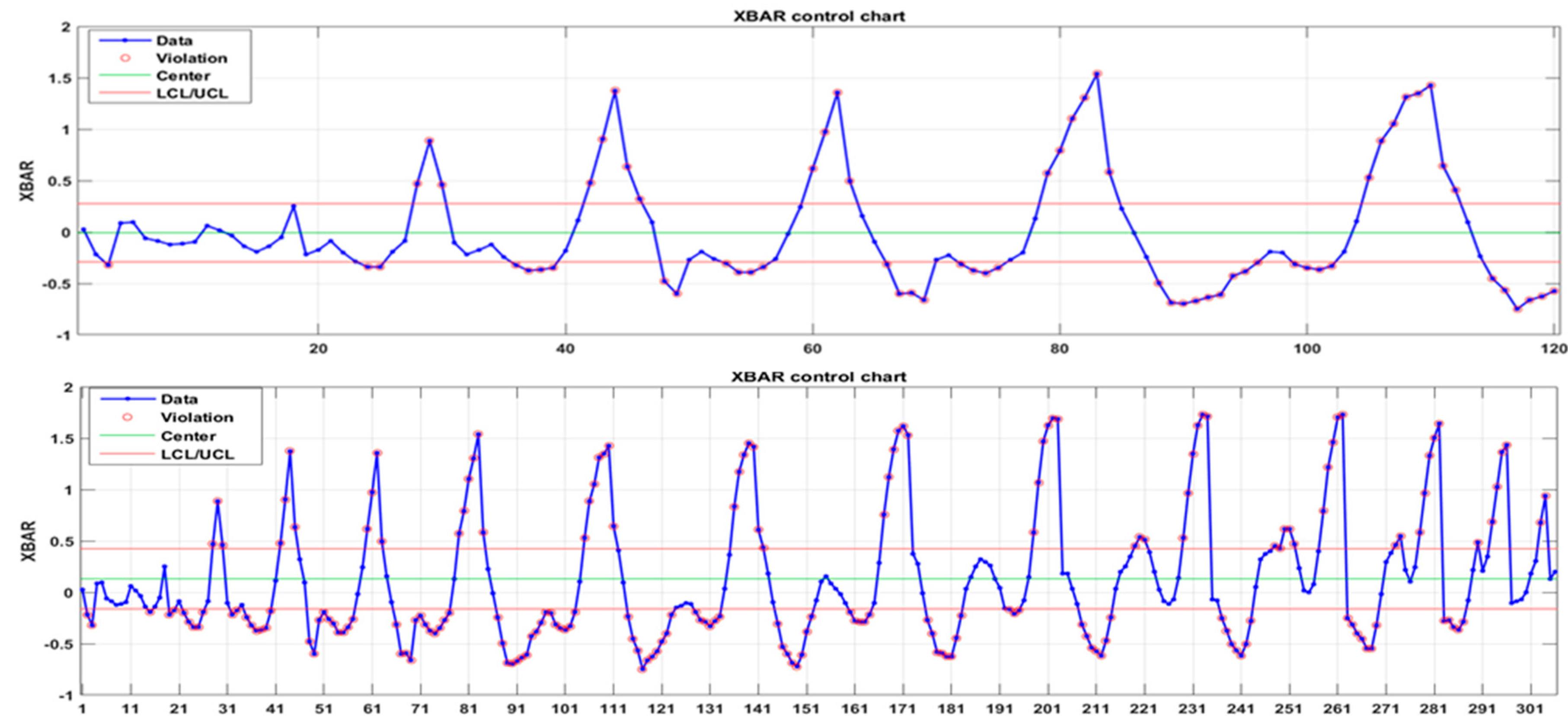
4.1. Temperature Trends

Figure 3a shows the differences between the mean air temperature measured at the landfill and the mean LST over the entire landfill recorded by satellites within the same hour as the air temperature. The differences show that the LST is consistently higher than the air temperature. Although the LST is expected to exceed air temperature somewhat as a normal result of subsurface processes in the landfill, differences that systematically increase over time indicate changes in the subsurface activities such as a smoldering or fire event.
The temperature variation shown in Figure 3a exhibits a periodic cycle due to seasonal changes, whereby the LST is higher during the summer or late spring and lower during the winter or late fall. The landfill maintains an average mean difference of approximately 6 °C (black straight line labeled “Mean 2000–2016”) between 2000 and 2016. From 2000 to 2011, the mean difference varies about 6 °C. After 2013, the mean difference appears to increase. Figure 3b shows the difference between the highest and lowest LSTs at the landfill (LST_max, LST_min). This difference shows an increasing trend similar to that of the mean difference, with relatively consistent values from 2000 to 2011, and higher values afterward. The higher temperature differences correspond to observed subsurface thermal events at the landfill. Figure 3b can shed light on some of the anomalies in the temperature change in the landfill as the difference between the lowest and the highest LSTs measured by remote sensing on the same day is increasing. However, this difference cannot tell us where the change is happening. With the extrapolation of LST data from the satellite images, it is possible to use the temperature trends to independently identify a recent SSE [21]. To determine the locations of hotspots, three areas were selected for closer study (with a focus on the spatial temperature distribution): the South Quarry (red) in the south area of the landfill, where most fire incidents have occurred and where the maximum temperature was recorded (both satellite and ground measurement); the Neck area (blue) to track any hotspots approaching the neck; and the North Quarry (green) adjacent to the radioactive waste area in the north part of the landfill. In Figure 4a, the landfill is divided into regions, using the mean LST as a baseline, to enable comparison of the deviations of these three different regions from the mean landfill temperature over 16 years. Figure 4 also depicts the history of heat elevation of the landfill during the study period. It reveals that during the 2000–2011 period, the all-regions temperature is clustered around the mean landfill temperature except for that of the upper region, which experienced elevated temperatures during the years 2004–2006 (Figure 4b in the lower middle part of Figure 4 shows the moving average).
Starting in 2013, compared to previous years, the whole landfill exhibited elevated temperatures. The lower region (South Quarry) continued to have the highest temperatures from 2013 to 2015. However, the northern region, which had maintained consistently low temperatures, experienced an increase in temperature of approximately 7 °C between 2013 and 2016 compared to the southern region. This can be clearly observed in the spike of elevated temperature in mid-2014 when the temperature of the North Quarry (green line in Figure 4) rises above the mean temperature of the landfill. The subsurface temperature in the southern area of the landfill continued to increase after 2011. During the years of the study, the maximum temperature was recorded in the lower region 81% of the time, and in the upper region only 12% of the time. Taking the upper region as a control, Figure 5 depicts the spatial temperature distribution in the landfill. Figure 5b shows that the lower region was measured to have the highest temperature, followed by the middle region. However, there were times where the upper region recorded the highest temperature. Figure 5a,c is analogous to Figure 5b with respect to the minimum and the mean temperature values.
Thus far, we have shown that by examining the landfill spatially, we were able to detect temperature anomalies (Figure 3) from satellite images, after which we detected regions with a higher temperature and revealed the historical health status of the landfill (Figure 4 and Figure 5). Next, we delve deeper to show changes at the pixel level and how the movement of the hot spots within the landfill can be traced during the years of the study. Figure 6 shows multitemporal maps (thermal maps) of the Bridgeton landfill in normalized scale (−8 to 8), in which the hotspots are easy to discern based on the LST. Figure 6a–l shows twelve snapshots of the LST hotspots from 2000 to 2011, respectively. These hotspots are consistently evident in the south and/or southeastern part of the South Quarry. Intermittent hotspots appear in the Neck area. Figure 6m–u shows nine snapshots of the LST hotspots from 2013 to 2016. These hotspots expanded to cover the entire southern portion of the landfill over the time period spanned by Figure 6.
Figure 7 shows locations that reached the highest (or near-highest) temperature values most frequently (frequency of maxima). The bar on the right side of the figure indicates the number of highest temperature occurrences at that spot. This information can be used to predict where internal fires are likely to occur. By continuously monitoring the frequency of maxima, we can identify new hotspots and track the beginning and end of SSEs. The red squares in Figure 7 indicate hotspots reported in February 2014 [23]. Some of the yellow squares correspond to other reported SSEs, such as that reported in 2012 [31].
The analysis of temperature trends shown above are based on the historical configuration of the Bridgeton Sanitary Landfill (North Quarry, Neck, and South Quarry) by the names used by the landfill operator. The purpose of this analysis was to monitor the movement of the hot spots in the landfill and the subsurface heat elevation to prevent them from reaching the North Quarry, which is adjacent to nuclear waste. The approach of an elevated heat area to the Neck serves as a warning and the need for action to be taken to prevent heat from spreading northward. However, for any landfill, the historical data collected and processed from satellite images can be grouped to identify regions for further study and to cluster them into three or more regions according to their temperature profiles. We used a simple method based on the areas of hottest, moderate, and cooler temperature to cluster the Bridgeton landfill into three regions. These newly define clusters (Figure 8) yield very similar results to those obtained above, and details of our analysis can be found in Appendix A. The blue cluster represents the hottest region in the landfill, i.e., the lower region in our study. Similarly, the green and yellow regions represent the middle and upper regions, respectively.

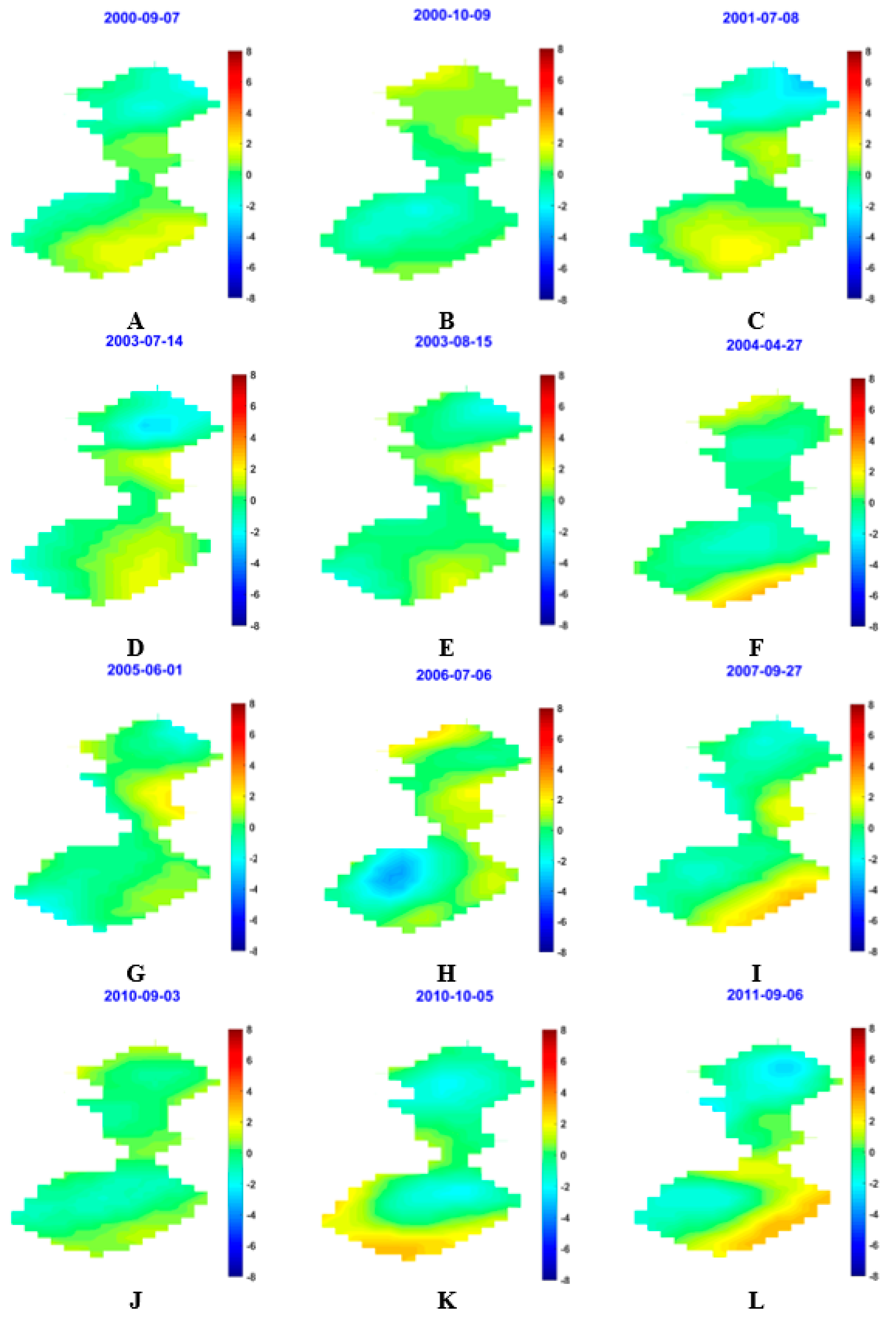
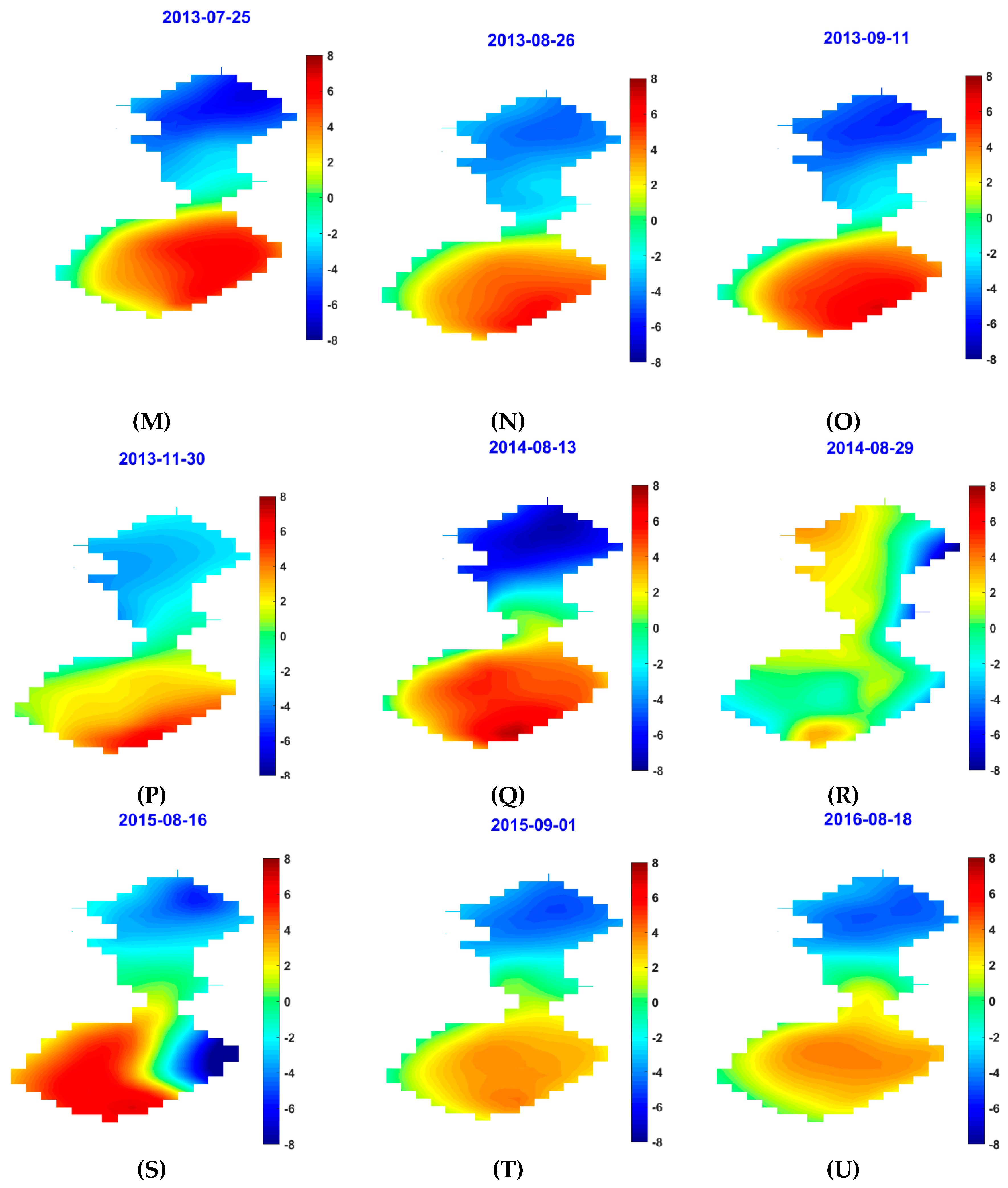
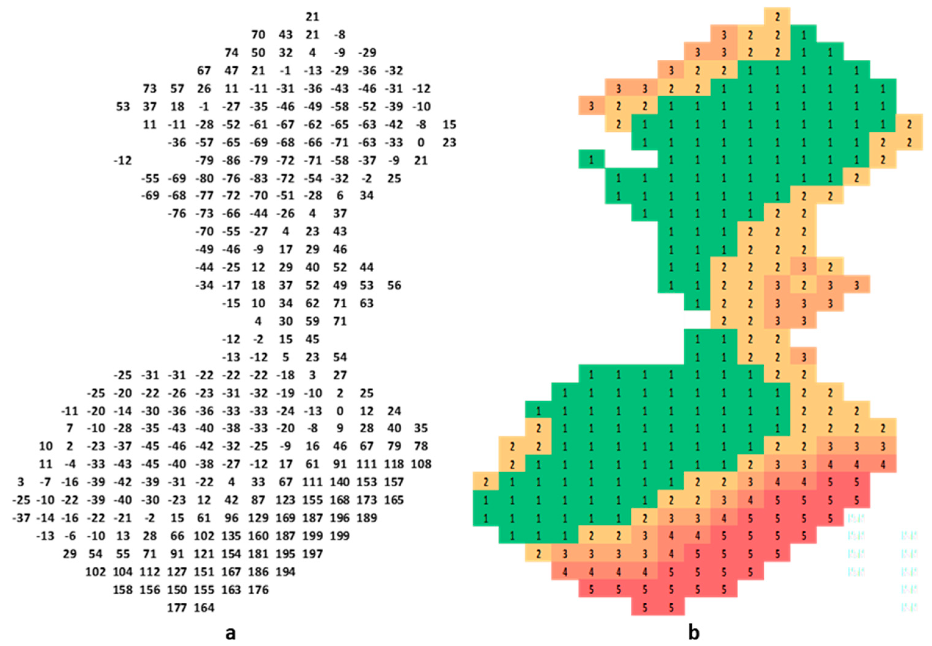
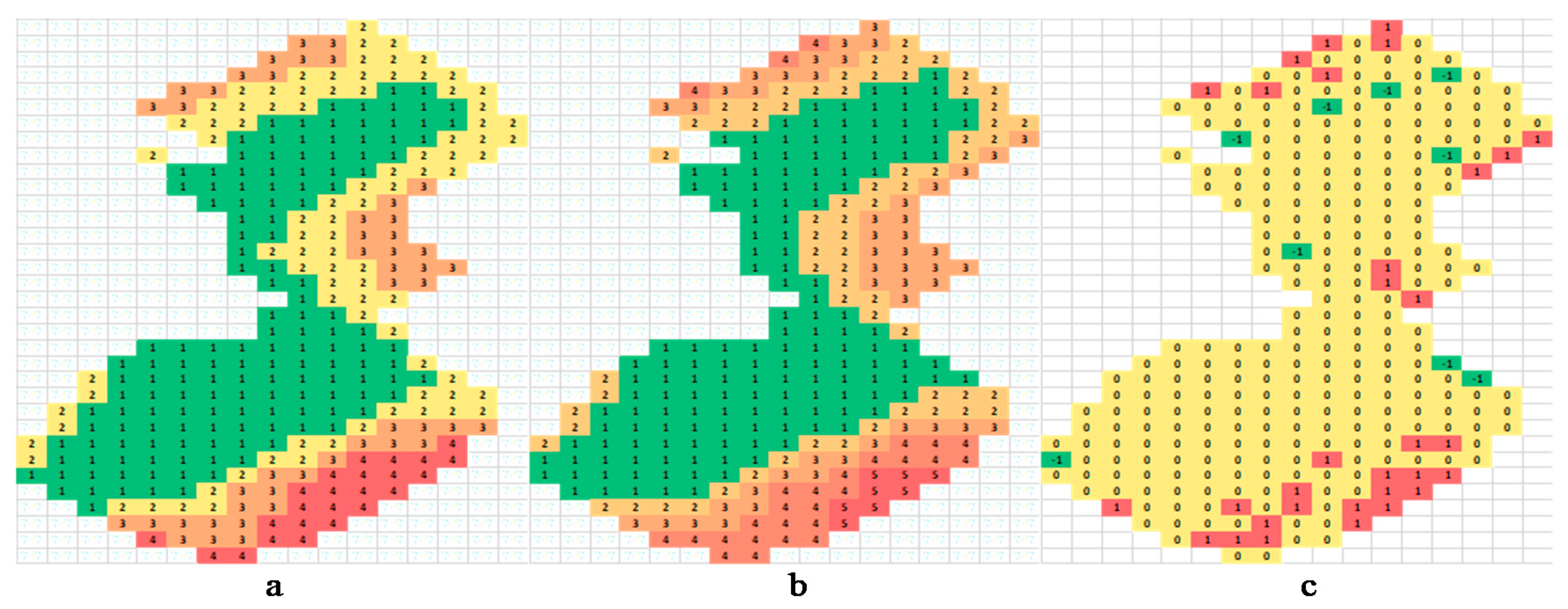
4.2. Behavior of the Landfill at Pixel Level in Both Spatial and Time Domains

Next, we investigated the behavior of each pixel in the LST observations by tracing the temperature profile for any given pixel during the 17 years of study. The observations were captured in different seasons of the year, with the summer observations usually having high temperatures, winter observations low temperatures, and spring and fall observations moderate temperatures. Therefore, it is difficult to infer any temperature anomalies. However, high ∆LSTs (LSTmax-LSTmin) for any given observation may indicate a temperature anomaly. Figure 3b shows the ∆LST values for all observations. The observations that exceed the mean temperature during the study years range from 6–18 °C and warrant further investigation to determine their location. To allow for comparison of different observations, they were normalized by subtracting the mean.
For each observation:
n = number of observations (LST thermal images) = 115.
p = index number of non-NaN-value (nonblank) pixels for a given image (i,j) = 306, where i, j are the number of rows and columns, respectively, in any given image, as shown in Figure 9a. For instance, (I = 27, j = 1) = P(1).
  t 1 =   time   of   image 1   jan   2000 t n = time   of   image 115   dec   2016 Δ T ij ( t ) =   ( T ij ( t )   T avg LF ( t ) ) .
where:
  • Δ T ij ( t ) is the normalized pixel (i,j) in any given image data;
  • T ij ( t ) is the recorded temperature in the LST observation in pixel (i,j) at time t;
  • T avg LF ( t ) is the landfill observation (image) average, which is given by Equation (6).
T avg LF ( t ) = i = 1 i = p T tp ( i )   p   ,   t = 1 : 115 .
We developed a heat index (HI) to classify the degree to which the temperature in each pixel deviated from the mean. Each classification was assigned an index number based on its variation from the mean, such that index (n) corresponds to an interval of (n) standard deviations from the mean, n = 1:5 as follows:
The HI for any given observation = HI(t) = −1   for Δ T ij ( t ) < 0
= 1   for 0 > Δ T ij ( t ) ≤ std(t)
= 2   for std(t) > Δ T ij ( t ) ≤ 2 std(t)
= 3   for 2std(t) > Δ T ij ( t ) ≤ 3 std(t)
= 4   for 3std(t) > Δ T ij ( t ) ≤ 4 std(t)
= 5   for Δ T ij ( t ) > 4 std(t)
All negative deviations are assigned index (−1) as they indicate temperatures below the mean. Figure 9b,c shows the normalized temperatures and equivalent HI values for image 79, dated 15 April 2011.
Now, all the observations are normalized to the mean, as shown in Figure 9b, and the equivalent HI (t) is calculated, as shown in Figure 9c. During this process, a master HI image is created to record the indices for each of the observations. The final HI is shown in Figure 10a, which ranges from −86 to 199. In addition, we added all the HI indices to an HI matrix of size (115,306), where each row represents one observation in one row vector and each column represents pixel values from t = 1 to t = 115.
As shown above, the same calculations were repeated for all the observations (from t = 1 on (“2010-01-19” to t = 115 on ”2016-12-08”) to obtain HI (t) values for all the observations. The end results are the HI image shown in Figure 10a and the HI matrix (not shown).
The HI obtained shows the temperature difference between all pixels in the landfill expressed in multiple standard deviations from the mean to avoid absolute temperature differences that could lead to the misinterpretation of thermal hot spots in different seasons. To study the temperature effect on each cell in the landfill during the study period, we calculated the accumulated heat index (AHI) as the cumulative columnwise sum of HI (CUMSUM):
AHI ( n = 115 , p = 306 ) = cumsum ( AH ( t ) )   .
Each row in the AHI is a cumulative sum of the preceding rows; therefore, the thermal status of the landfill can be inferred and plotted at any given time during the study period. The last row in the AHI is equivalent to the result shown in Figure 10a reshaped into a row vector.
Columns in the AHI (p = 1: p = 306) represent pixel locations in the landfill, as shown in Figure 9a. By tracing each column, the thermal status and behavior of a specific location can be determined from January 2000 to December 2016. To do so, new indices must be extracted based on the cumulative sum of the AHI. These new indices can be calculated as described above at k-standard deviation intervals using the following equation:
I =   AHI ( t , p ) > [ Mean AHI + ( K ×   std AHI   ) ] ,
where K = 1, 2, 3, 4
  • I = 1 for all negative indices (lowest);
  • I = 2, 3, 4 for intervals 2, 3, 4 standard deviations;
  • I = 5, for AHI (t,p) >   Mean AHI + ( 4   std AHI   )   − (highest),
where Mean AHI is the mean of all indices in the AHI and can be calculated as follows:
Mean AHI =   p = 1 p = 306 t = 1 t = 115 AH ( t ) n   ×   p ,
and std AHI   is the standard deviation of the AHI column means. The overall heat index (I) of the landfill for the study period is obtained as explained above and shown in Figure 10b.
By the end of the study period, we observed that 10% of the landfill was experiencing high temperature, mainly in the southwest of the South Quarry, and 25% of the landfill was showing temperatures three times greater than the standard deviation. As shown in Figure 11a, cells/pixels with I = 5 tend to exhibit increasing behavior during the period of study. The pixels in Figure 11b with I = 4 show the same increasing trend at lower levels of standard deviation. As indicated in Figure 11a,b, the heat elevation in this area of the landfill is consistent for many years and is also expanding to neighboring areas. The other I (1–3) indices show different trends, with some pixels showing an increasing trend and others a decreasing trend for the same index. However, all the rising indices reach their peaks beginning in year 2010 and maintain that level until mid-2013. I = 3 in Figure 11c shows the same increasing trend at different levels of standard deviation until 2013, but some pixels continue to increase while others start to decrease. A few I = 2 pixels in Figure 11d continue to rise to nearly two standard deviations and most are above one standard deviation. However, some pixels show decreasing temperatures until 2013 and then start to rise again. Similarly, pixels with the index I = 1 pose no concern as they remain around the mean. We are only concerned with the beginning of the temperature rise at the end of 2013 in Figure 11e.
The SSE reported in 2010 can be inferred from the rising temperature indices shown in Figure 11, wherein all pixels/cells reach peak values beginning in 2010, which they retain until the end of 2011, except for I 4 and I 5, which continue to increase rapidly [21,23]. Following the same reasoning described above, Figure 12a,b shows the thermal status of the landfill between February 2010 and September 2011 (19 months), in which the locations of all pixels that continue to rise in temperature are evident. Figure 12c shows the location and degree of difference over the 19 months. A comparison of Figure 10b, which shows the thermal status of landfill by the end of 2016, with Figure 12b reveals that there is greater heat elevation and that it has continued to spread in the southern part of the landfill.
Figure 13 shows a plot of the X-bar (XBAR) control chart for the AHI matrix (115,306), which contains indices 1–5 for all years of the study (time domain) and for all pixels (spatial domain). The XBAR chart detects violations based on those that exceed ±3 σ between the two red lines in Figure 13a,b. We ignore violations below −3 σ as they indicate low temperature, which is not a matter of concern. Figure 13a shows violations in the time domain (observations from January 2000 to December 2016), of which there were many during the period of study. Similarly, Figure 13b shows violations at the pixel level by matching the pixels in Figure 13b with I (3–5). The x-axes indicate the pixel locations depicted in Figure 9a.

5. Discussion and Conclusions

Surprisingly, there are few published papers regarding the remote monitoring of landfill fires. To our knowledge, this is the first study to evaluate the performance of an interdisciplinary remote sensing method in monitoring and predicting fire events in the USA. Because of the closures of many landfills and other disposal facilities over the past 40 years [32], the number of neglected waste sites has increased along with the chance of subsurface events. These closed and abandoned waste sites around the USA must be monitored for subsurface activities that can lead to above-surface hazards. Remote sensing can be used to address this problem and locate hotspots by monitoring the thermal signature of these waste sites. Hotspots can be an indication of the potential for fire that can threaten human health and the environment. In this paper, a noninvasive method is proposed for monitoring temperature by the collection of sufficient information to enable the timely detection of subsurface events. To reach this goal, in this study, temperature data contained in the Landsat satellite images (USGS Explorer archives) were converted into a more workable format and then analyzed. As presented in the results section, the location of hotspots at Bridgeton Sanitary Landfill, Missouri, were successfully detected and monitored. Multitemporal LST thermal maps were plotted for this case study, whereby a large difference between the LST and air temperature provided a warning of the need to investigate. We controlled for seasonality by measuring temperatures at different areas in the same landfill at the same time. This technique can effectively detect most hotspots and the results have been verified by the consultant report [21,23]. The use of satellite remote sensing techniques for the detection of possible fires in landfills has great practical significance when there is no landfill data available or in the detection of illegal waste dumps. The 30-m spatial resolution of the thermal band can detect most of the substantial hotspots as these usually last for months and their generated heat propagates both vertically and horizontally for distances that are detectable by satellite infrared sensors. However; this technique is limited by the validity and availability of imagery because of cloud cover and the length of time between revisits of the satellite to the same place (every 16 days), respectively. The depth of the hotspot is also an important factor. For hotspots of the same size, the deeper the hotspot is, the smaller the increase in LST temperature. Given the availability of public data from the USGS Explorer satellite images database, the proposed method can be applied to any landfill in USA territory to predict subsurface thermal events.
Future work should include the incorporation of this method into a formal satellite-based landfill monitoring system that uses thermal infrared observations from Landsat satellites to assess the thermal state of any landfill surface and identify anomalous thermal patterns and changes of any USA landfill. This information can also be used to issue warnings regarding the potential for landfill fires. The results generated by this study provide perfect data input for the monitoring system and includes algorithms for efficient satellite image classification and physically based land-surface temperature retrieval. Thermal remote sensing is an effective tool for monitoring the internal activities of landfills and provides a reliable method for predicting fire outbreaks and preventing possible environmental disasters.

Author Contributions

Investigation, H.A., M.G.R.F. and S.S.; Supervision, R.N.; Writing—original draft, F.H., M.E.K., J.E. and N.B.; Writing—review & editing, R.W.P. All authors have read and agreed to the published version of the manuscript.

Funding

This work was funded by the US Department of Agriculture (USDA) Solid Waste Management Grant Programs.

Conflicts of Interest

The authors declare no conflict of interest.

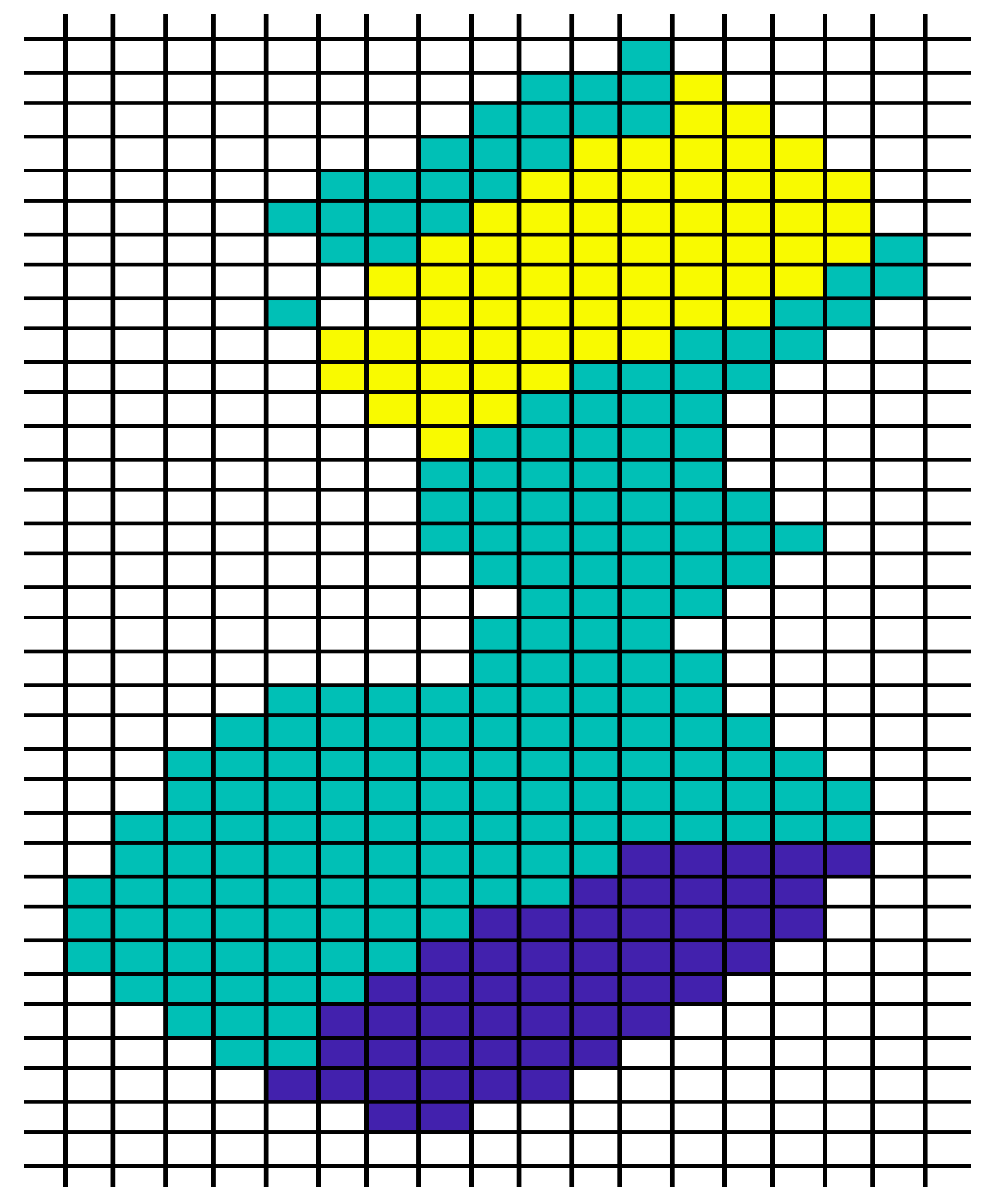
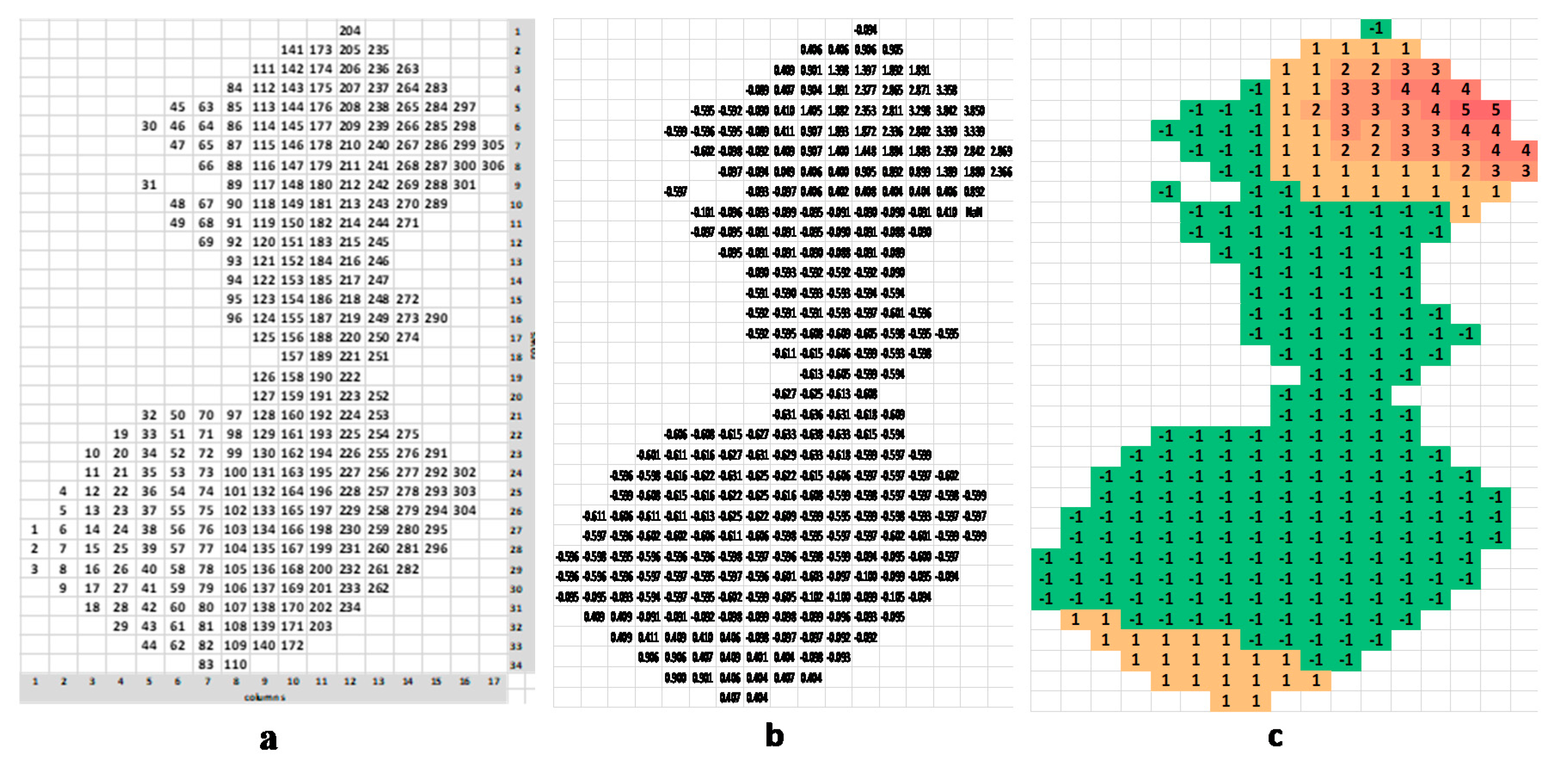
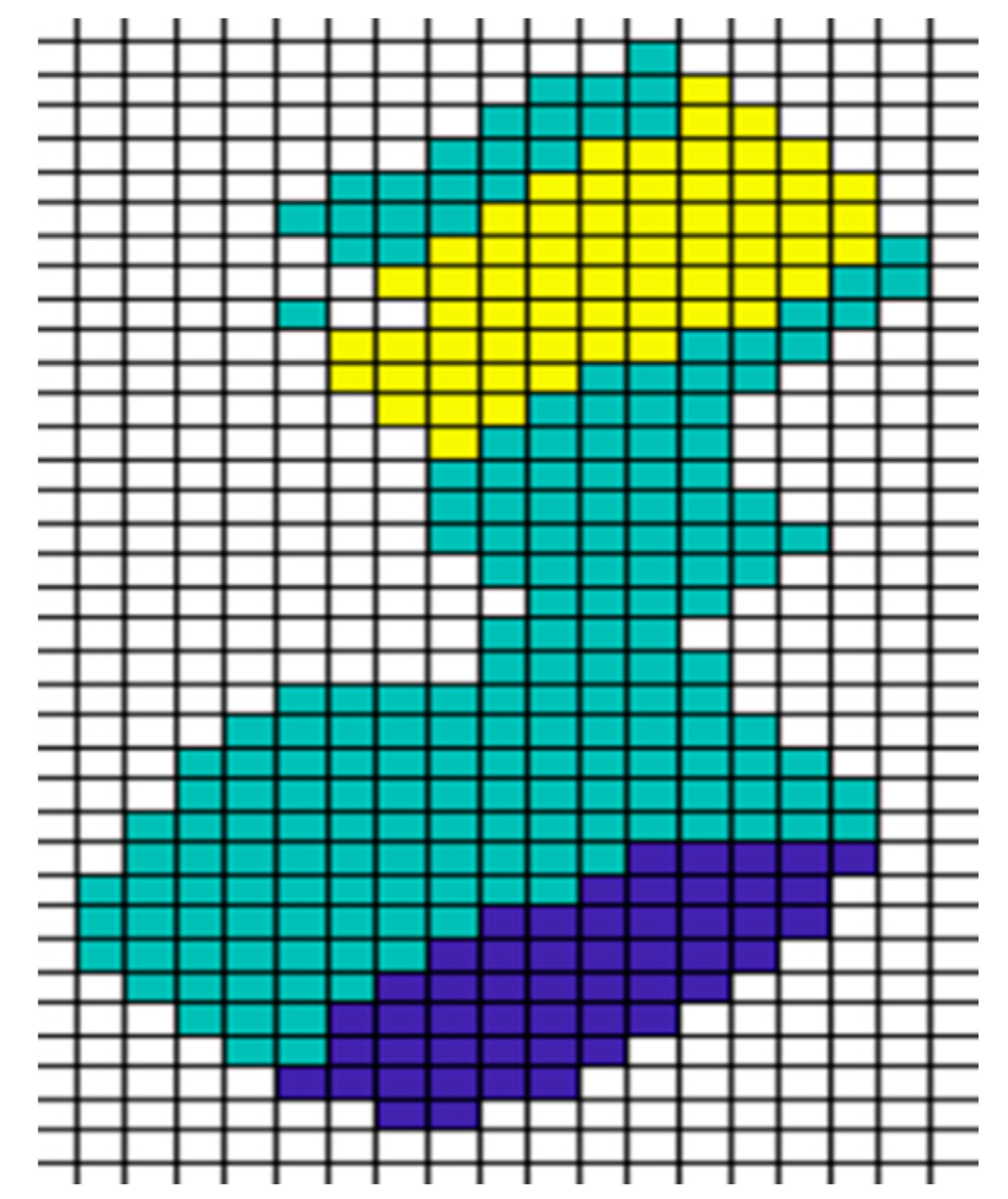
Appendix A. Clustering the Landfill Based on Its Temperature

The original landfill configuration, shown in Figure 5, used shapefiles with following number of pixels:
  • Number of cells for whole landfill = 306
  • Number of cells South quarry (lower region) = 180
  • Number of cells Neck area (middle region) = 72
  • Number of cells North quarry (upper region) = 54
To apply this methodology for any landfill, landfills can be clustered based on their temperature profile. This will help in focusing on regions that have higher temperature or substantial temperature differences in the same landfill. The temperature profile can be built from the satellite observations for any number of years or months. Doing so, we bear in mind that subsurface heat elevation or smoldering events will last long (persistent for some time) if it is not treated by the landfill operators and its effect will be shown in all subsequent satellite images. For Bridgeton landfill, we collected 115 satellite observations from year 2000 to 2016 as shown in Table 1. These observations construct a temperature time series; therefore; to create new clusters we need to consider observation time from image 1 at ti = 1 until te = 115 for all the image pixels (i, j). Clustering can be done using any of the clustering techniques such as k-means or PCA. However, we clustered the landfill based on the deviation from the mean as follows:
t i = initial   time   (   image   1 )
t e = end   time   (   image   115 )
n = number of observations
T ij ( t ) = Temperature   at   cell   i , j   and   time   t
  • T avg _ LF ( t ) = mean landfill temperature at time t
  • Δ ij ( t ) =   ( T ij ( t )   T avg _ LF ( t ) ) for cells, i,j are the pixel coordinates
  • mean = ( t i t e Δ ij (t))/n
STD   = Standard   deviation   ( t i t e Δ ij ( t ) )
Then calculating:
mean STD   yields   Cluster   1   ( yellow )
mean ¯ +   STD   yields   Cluster   2   ( green )
Cluster 3 is all the rest (blue). The resultant cluster is shown in Figure A1.
Figure A1. Clustering Bridgeton landfill based on the mean and standard deviation of all observations.
Applsci 10 06801 g0a1
Cluster 3 (blue) is equivalent to lower part or South quarry where the highest temperature is recorded most of the time, cluster 2 (green) similar to middle region where moderate temperature is recorded and the cluster 1 (yellow) is the upper region where the lowest temperature is recorded most of the time. The shapefiles and the number of cells for each region has been changed to:
  • Number of cells for whole landfill = 306
  • Number of cells South quarry (lower region) = 52
  • Number of cells Neck area (middle region) = 190
  • Number of cells North quarry (upper region) = 64
This analysis is simple and helps to identify the regions of concern and the percentage of landfill going under different heat elevation levels; for instance, about 17% of the landfill is under subsurface heat elevation (blue), about 62% is under moderate heat elevation (green) and 21% of the landfill is under normal heat conditions. Reproducing spatial temperature profiles was previously obtained in Figure 3 and Figure 4, based on new clusters that show similar heat trends. In addition, using k-means clustering resulted in a similar classification.

References

  1. You, H.; Ma, Z.; Tang, Y.; Wang, Y.; Yan, J.; Ni, M.; Cen, K.; Huang, Q. Comparison of ANN (MLP), ANFIS, SVM, and RF models for the online classification of heating value of burning municipal solid waste in circulating fluidized bed incinerators. Waste Manag. 2017, 68, 186–197. [Google Scholar] [CrossRef]
  2. Hanson, J.L.; Liu, W.-L.; Yesiller, N. Analytical and numerical methodology for modeling temperatures in landfills. In GeoCongress 2008: Geotechnics of Waste Management and Remediation; American Society of Civil Engineers (ASCE): New Orleans, LA, USA, 2008; pp. 24–31. [Google Scholar]
  3. Yeşiller, N.; Hanson, J.L.; Liu, W.-L. Heat generation in municipal solid waste landfills. J. Geotech. Geoenviron. Eng. 2005, 131, 1330–1344. [Google Scholar] [CrossRef] [Green Version]
  4. Faitli, J.; Magyar, T.; Erdélyi, A.; Murányi, A. Characterization of thermal properties of municipal solid waste landfills. Waste Manag. 2015, 36, 213–221. [Google Scholar] [CrossRef] [PubMed]
  5. Faitli, J.; Magyar, T.; Romenda, R.; Erdélyi, A.; Boldizsár, C. Laying the Foundation for Engineering Heat Management of Waste Landfills. Environ. Res. J. 2017, 11, 323–348. [Google Scholar]
  6. ATSDR. Landfill Gas Primer: An Overview for Environmental Health Professionals; United States Agency for Toxic Substances and Disease Registry (ATSDR): Atlanta, GA, USA, 2001.
  7. Brune, M.; Ramke, H.; Collins, H.; Hanert, H. Incrustation processes in drainage systems of sanitary landfills. In Proceedings of the 3rd International Landfill Symposium, Cagliari, Italy, 4–8 October 1999; pp. 999–1035. [Google Scholar]
  8. Döll, P. Desiccation of mineral liners below landfills with heat generation. J. Geotech. Geoenviron. Eng. 1997, 123, 1001–1009. [Google Scholar] [CrossRef]
  9. El-Fadel, M.; Findikakis, A.; Leckie, J. Numerical modelling of generation and transport of gas and heat in landfills I. Model formulation. Waste Manag. Res. 1996, 14, 483–504. [Google Scholar] [CrossRef]
  10. Pirt, S. Aerobic and anaerobic microbial digestion in waste reclamation. J. Appl. Chem. Biotechnol. 1978. [Google Scholar]
  11. McBean, E.A.; Rovers, F.A.; Farquhar, G.J. Solid Waste Landfill Engineering and Design; Prentice Hall: New York, NY, USA, 1995. [Google Scholar]
  12. Southen, J.; Rowe, R.K. Modelling of thermally induced desiccation of geosynthetic clay liners. Geotext. Geomembr. 2005, 23, 425–442. [Google Scholar] [CrossRef]
  13. Yoshida, H.; Rowe, R. Consideration of landfill liner temperature. In Proceedings of the Sardinia 2003, Ninth International Waste Management and Landfill Symposium S, Margherita di Pula, Cagliari, Italy, 6–10 October 2003. [Google Scholar]
  14. Kwarteng, A.; Al-Enezi, A. Assessment of Kuwait’s Al-Qurain landfill using remotely sensed data. J. Environ. Sci. Health Part A 2004, 39, 351–364. [Google Scholar] [CrossRef] [PubMed]
  15. Shaker, A.; Yan, W.Y. Trail road landfill site monitoring using multitemporal Landsat satellite data. In Proceedings of the Canadian Geomatics Conference 2010 and ISPRS COM I Symposium, Calgary, AB, Canada, 14–18 June 2010. [Google Scholar]
  16. Hall, D.; Drury, D.; Keeble, R.; Morgans, A.; Wyles, R. Review and Investigation of Deep-Seated Fires within Landfill Sites; Environment Agency: Bristol, UK, 2007.
  17. Jafari, N.H. Elevated Temperatures in Waste Containment Facilities; University of Illinois at Urbana-Champaign: Champaign, IL, USA, 2015. [Google Scholar]
  18. Youmaran, K. We Didn’t Start the Fire: The Current Outlook of the Bridgeton Landfill and Its Implications for Missourians. J. Environ. Sustain. Law 2015, 22, 365. [Google Scholar]
  19. Kret, J.; Dame, L.D.; Tutlam, N.; DeClue, R.W.; Schmidt, S.; Donaldson, K.; Lewis, R.; Rigdon, S.E.; Davis, S.; Zelicoff, A. A respiratory health survey of a subsurface smoldering landfill. Environ. Res. 2018, 166, 427–436. [Google Scholar] [CrossRef] [PubMed]
  20. Alvarez, R. The West Lake Landfill: A Radioactive Legacy of the Nuclear Arms Race; Institute for Policy Studies: Washington, DC, USA, 2013. [Google Scholar]
  21. Thalhamer, T. Subsurface Chemical Processes at the Bridgeton Landfill; Hammer Consulting Service: Cameron Park, CA, USA, 2013. [Google Scholar]
  22. Timothy, D. Stark, T.T. Bridgeton Landfill North Quarry Contingency Plan; Quality, D.O.E., Ed.; Missouri Department of Natural Resources: Jefferson City, MO, USA, 2013.
  23. Thalhamer, T. Data Evaluation of the Subsurface Smoldering Event at the Bridgeton Landfill; Hammer Consulting Service: Cameron Park, CA, USA, 2015. [Google Scholar]
  24. USGS. Landsat 8 (L8) Data Users Handbook, 2nd ed.; United States Geological Survey (USGS): Reston, VA, USA, 2016.
  25. Weng, Q.; Lu, D.; Schubring, J. Estimation of land surface temperature–vegetation abundance relationship for urban heat island studies. Remote Sens. Environ. 2004, 89, 467–483. [Google Scholar] [CrossRef]
  26. Van de Griend, A.; OWE, M. On the relationship between thermal emissivity and the normalized difference vegetation index for natural surfaces. Int. J. Remote Sens. 1993, 14, 1119–1131. [Google Scholar] [CrossRef]
  27. Zhang, J.; Wang, Y.; Li, Y. A C++ program for retrieving land surface temperature from the data of Landsat TM/ETM+ band6. Comput Geosci. 2006, 32, 1796–1805. [Google Scholar] [CrossRef]
  28. Sobrino, J.A.; Jiménez-Muñoz, J.C.; Paolini, L. Land surface temperature retrieval from LANDSAT TM 5. Remote Sens. Environ. 2004, 90, 434–440. [Google Scholar] [CrossRef]
  29. Li, Z.-L.; Wu, H.; Wang, N.; Qiu, S.; Sobrino, J.A.; Wan, Z.; Tang, B.-H.; Yan, G. Land surface emissivity retrieval from satellite data. Int. J. Remote Sens. 2013, 34, 3084–3127. [Google Scholar] [CrossRef]
  30. Mahmood, K.; Batool, S.A.; Chaudhry, M.N. Studying bio-thermal effects at and around MSW dumps using Satellite Remote Sensing and GIS. Waste Manag. 2016, 55, 118–128. [Google Scholar] [CrossRef] [PubMed]
  31. Archived Reports: Bridgeton Sanitary Landfill. Available online: https://dnr.mo.gov/bridgeton/BridgetonSanitaryLandfillReports.htm (accessed on 4 June 2020).
  32. U.S. Fire Administration. Landfill Fires: Their Magnitude, Characteristics, and Mitigation; U.S. Fire Administration: Emmitsburg, MA, USA, 2002.
Figure 1. Outlines of Bridgeton landfill areas [20].
Applsci 10 06801 g001
Figure 2. (a) Bridgton Landfill, divided by regions, and the surrounding area. (b) Latitude and longitude of the landfill and overlay of regions on Google Earth.
Applsci 10 06801 g002
Figure 3. (a) Comparison of mean LSTs and mean air temperatures and (b) a comparison of the maximum and minimum LSTs for given image dates for Bridgeton landfill.
Applsci 10 06801 g003
Figure 4. Relative temperature differences in the 17-year span for Bridgeton Sanitary Landfill, Missouri. (a) Mean LST of different regions within the landfill; (b) LST generated from moving average approach.
Applsci 10 06801 g004
Figure 5. Taking the upper region as a ”control” and comparing it with the lower/middle regions.
Applsci 10 06801 g005
Figure 6. Thermal map of Bridgeton landfill displaying LST in degree Celsius (°C) at various times and dates from 2000–2011: 7 September 2000 (A); 9 October 2000 (B); 8 July 2001 (C); 14 July 2003 (D); 15 August 2003 (E); 27 April 2004 (F); 1 June 2005 (G); 6 July 2006 (H); 27 September 2007 (I); 3 September 2010 (J); 5 October 2010 (K); 6 September 2011 (L); 25 July 2013 (M); 26 August 2013 (N); 11 September 2013 (O); 30 November 2013 (P); 13 August 2014 (Q); 29 August 2014 (R); 26 April 2015 (S); 12 May 2015 (T); 30 May 2016 (U).
Applsci 10 06801 g006aApplsci 10 06801 g006b
Figure 7. Location of frequency of maxima/near-maxima around the landfill site of Bridgeton, Missouri. The bar on the right side indicates the frequency of occurrence of maximum temperature at that point.
Applsci 10 06801 g007
Figure 8. Clustering of Bridgeton landfill based on means and standard deviations of all observations.
Applsci 10 06801 g008
Figure 9. (a) Landfill pixels numbered from 1–306; (b) normalized data of observation 15 April 2011; (c) equivalent HI. (Blank squares = NaN values (nonblank)).
Applsci 10 06801 g009
Figure 10. (a) Accumulated heat index (AHI) and (b) equivalent I for the entire landfill by end of 2016.
Applsci 10 06801 g010
Figure 11. (a,b,c) I (5, 4, 3), respectively, showing an increasing trend; (d) I = 2; (e) I = 1.
Applsci 10 06801 g011
Figure 12. Thermal states of the landfill in (a) February 2010 and (b) September 2011, and (c) thermal status difference.
Applsci 10 06801 g012
Figure 13. XBAR control chart showing violations, i.e., exceeding ±3 σ (a) per observation and (b) per pixel.
Applsci 10 06801 g013
Table 1. Brightness temperature constant values for use with Equation (1).
ConstantK1K2
UnitsW/ (sr m2 µm)kelvin
L5 TM607.761260.56
L8 TIR774.891321.08

