An Improved Calibration Method for the Misalignment Error of a Triaxial Magnetometer and Inertial Navigation System in a Three-Component Magnetic Survey System

Abstract

In order to calibrate the misalignment error of a triaxial magnetometer and an inertial navigation system in a three-component magnetic survey system, an improved method with easy realization is proposed in this paper. We establish the misalignment error model based on Euler’s theorem. We transform the calibration of misalignment error into estimating calibration parameters to minimize the value of objective function. Then, the nonlinear least squares method is used to estimate the calibration parameters. In the simulation experiment, the deviation between the value and the preset value is within 1 nT. In the field experiment, the fluctuation value of the x, y, and z components reduce to 1.09%, 0.92%, and 1.28%, respectively. The absolute deviation values are reduced to 0.72%, 0.70%, and 0.81% and the standard deviation value are reduced to 0.74%, 0.71%, 0.86%, respectively. The proposed method has advantages of high operability and precision as compared with existing methods.

1. Introduction

A three-component magnetic survey system is composed of a triaxial magnetometer and an inertial navigation system (INS) and is widely used in resource exploration [1], magnetic anomaly detection [2], and geomagnetic aid for navigation [3,4]. An INS is used to provide attitude information to restore three-component magnetic data to a geographic coordinate system. The accuracy of the restoration process is affected by the accuracy of the INS and the misalignment error of the system. There have been many research achievements made in error correction of a magnetometer [5,6,7] and improving the accuracy of an INS [8,9,10]. In 1997, Primdahl proposed a method to align the magnetometer and star sensor [11]. However, research on misalignment error is still relatively weak. Theoretically, 1° misalignment error results in thousands of nT errors in the measurement results [12]. According to the above studies, calibration of misalignment error is necessary, and it has been classified into a physical method and an algorithm calibration method. Since the physical method is difficult to implementation and has low precision, we need to develop an algorithm method to calibrate misalignment error. In recent years, some achievements for calibrating misalignment error have appeared in the research.

A class of method called “dot product invariance” (DPI) was proposed in 2012, based on the fact that the vector dot product of geomagnetic field and gravitational field is constant [13]. The method calibrates the misalignment error between gravimeter and magnetometer by using an auxiliary vector to simulate the gravitational field. The calibration accuracy of this method is easily affected by the selection of auxiliary vectors, which is reduced when there is a difference between the auxiliary vector and the gravitational field.

Zhu proposed a method, in 2017, that combined the ellipsoid fitting method with the DPI method [14,15]. This method could calibrate the misalignment error between an accelerometer and a magnetometer effectively, but it had the same defects as the DPI method.

Gao proposed a new method, in 2019, which was based on the fact that the trajectories of magnetic data obtained by a magnetometer which rotated in the same attitude under different background magnetic field were parallel to each other [16]. This method solved the problem of the DPI method that was sensitive to the selection of auxiliary vector. However, it needed at least two sets of data rotated about different axes to complete parameter optimization. When replacing the rotating plane, the misalignment error could change due to improper operation.

Consider the deficiencies of the above methods, we propose an improved method to calibrate the misalignment error. The misalignment error of magnetometer and INS is analyzed and modeled firstly. Then the principle of the calibration method is introduced. Finally, the feasibility and accuracy of the proposed method are verified by simulation and field experiment.

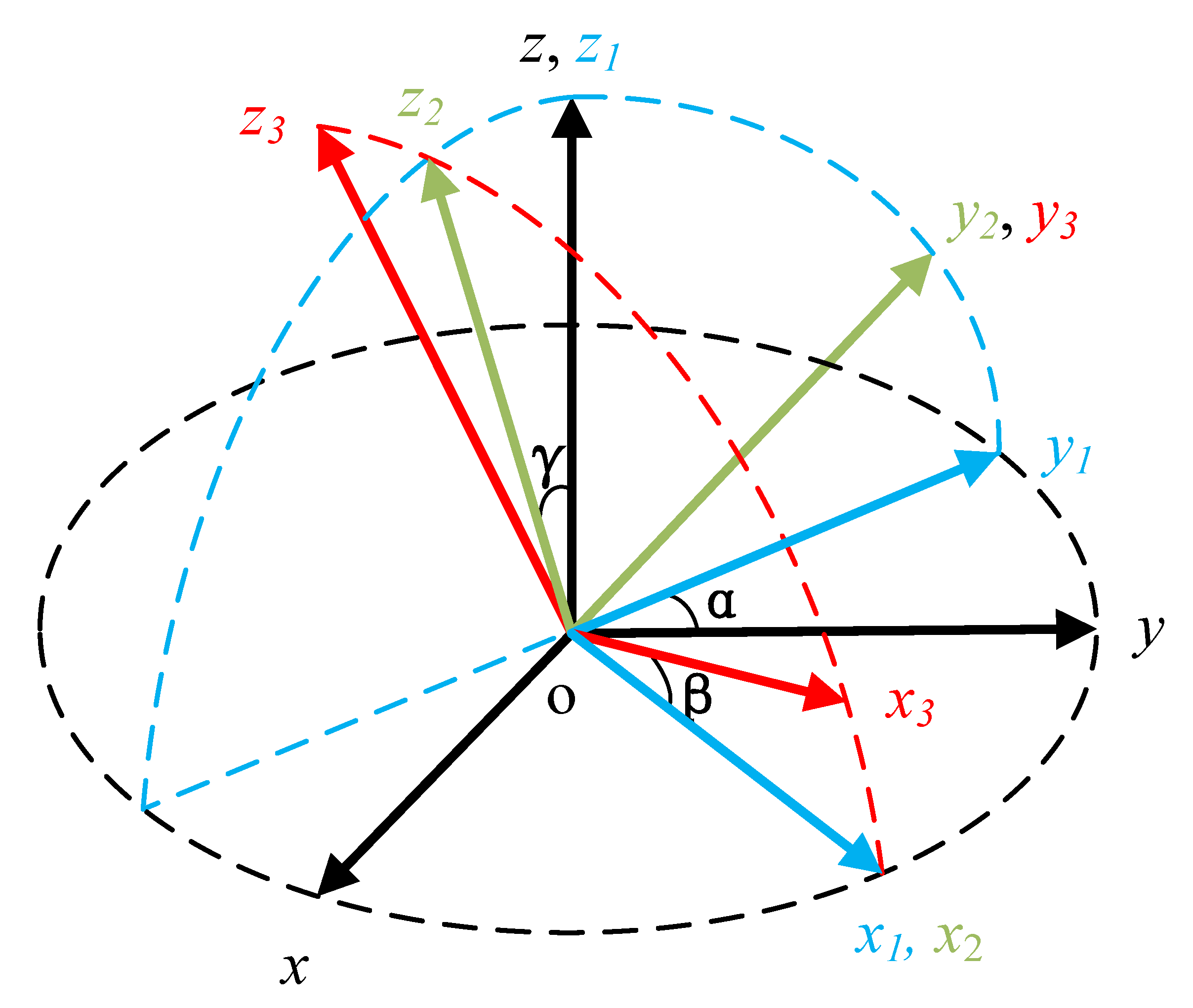
2. Misalignment Error Analyses

We define two orthogonal coordinate systems to describe the misalignment error as follows: the INS coordinate system $\left(o-x_i{y}_i{z}_i\right)$ and the magnetometer coordinate system $\left(o^{\prime }-x_m{y}_m{z}_m\right)$. As shown in Figure 1, the three-axis misalignment between a magnetometer coordinate system and an INS coordinate system caused by misalignment error is reflected.

According to Euler’s theorem [17], the rotation transformation between two orthogonal coordinate systems can be described by a 3 × 3 rotation matrix R. Then, the misalignment error calibration can be transformed into solving the rotation matrix R.

$$\left[\begin{array}{c}{X}_i\\ Y_i\\ Z_i\end{array}\right]=\mathit{R}\cdot \left[\begin{array}{c}{X}_m\\ Y_m\\ Z_m\end{array}\right]$$

(1)

We set a matrix $\mathit{S}$ as follows:

$$\mathit{S}=\left[\begin{array}{ccc}0& -s_z& s_y\\ s_z& 0& -s_x\\ -s_y& s_x& 0\end{array}\right]$$

(2)

Then, we can express the rotation matrix R as:

$$\mathit{R}={(\mathit{I}-\mathit{S})}^{-1}\cdot (\mathit{I}+\mathit{S})$$

(3)

where I denote the unit matrix.

3. Calibration Method

This method is based on the following three principles:

(a) The trajectory of the measurement data is a circle if the triaxial magnetometer rotates about an axis in a steady magnetic field. Two trajectories of the measurement data obtained by the same magnetometer rotating about the same axis under different background magnetic fields are also two circles which are parallel to each other.

(b) The tangent vectors of two parallel circles at the same phase are parallel.

(c) The normal vectors of two parallel circles are parallel.

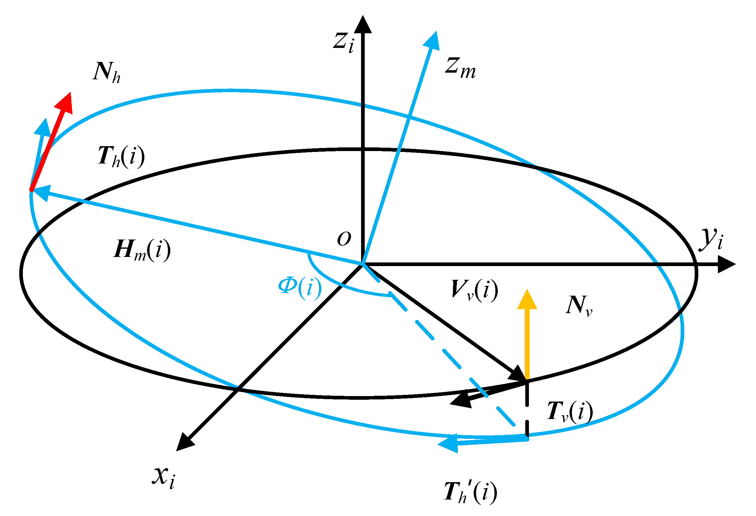
3.1. Virtual Auxiliary Vector

In order to determine the position relationship between an INS coordinate system and a magnetometer coordinate system, we assume a virtual vector $\mathit{V}$ to expand the INS’s angle to magnetic value.

$$\mathit{V}=\left[\begin{array}{c}{v}_x\\ v_y\\ v_z\end{array}\right]$$

(4)

We set $\mathit{V}$ as a different background magnetic field in the INS coordinate system. The INS coordinate system is based on a geographic coordinate system, i.e., the x-, y- and z-axes point east, north, and up, respectively. The auxiliary correction data can be obtained by rotating $\mathit{V}$. Euler’s rotation method is used to generate auxiliary calibration data. A vector can be rotated to any angle by three rotations around a single coordinate axis [18,19]. These three rotations are as follows: rotating around the z-, x- and y-axes, respectively. They can be expressed as:

$${\mathit{E}}_x=\left[\begin{array}{ccc}1& 0& 0\\ 0& \cos \gamma & -\sin \gamma \\ 0& \sin \gamma & \cos \gamma \end{array}\right]$$

(5)

$${\mathit{E}}_y=\left[\begin{array}{ccc}\cos \beta & 0& \sin \beta \\ 0& 1& 0\\ -\sin \beta & 0& \cos \beta \end{array}\right]$$

(6)

$${\mathit{E}}_z=\left[\begin{array}{ccc}\cos \alpha & -\sin \alpha & 0\\ \sin \alpha & \cos \alpha & 0\\ 0& 0& 1\end{array}\right]$$

(7)

where $\alpha ,\beta$ and $\gamma$ denote heading, roll, and pitch angles. ${\mathit{E}}_x,{\mathit{E}}_y$ and ${\mathit{E}}_z$ denote the rotation matrix around the x-axis, y-axis, and z-axis, respectively.

According to Euler rotation method, the analytical order of INS attitude data is shown in Figure 2:

$$o-xyz\to o-x_1{y}_1{z}_1\to o-x_2{y}_2{z}_2\to o-x_3{y}_3{z}_3$$

We set the virtual vector as the magnetic field value of the geographic coordinate system. Therefore, we can generate the auxiliary correction dates as Equations (8) and (9).

$$\mathit{E}={\mathit{E}}_y\cdot {\mathit{E}}_x\cdot {\mathit{E}}_z$$

(8)

$${\mathit{V}}_v=\mathit{E}\cdot \mathit{V}$$

(9)

where the “$\cdot$” donates the matrix multiplication.

We can consider that the virtual vector and the real geomagnetic field are two different stable background magnetic fields. The auxiliary correction data and the measured data are obtained from the same rotation in these two stable background magnetic fields. The trajectories of ${\mathit{V}}_v$ and measured magnetic data ${\mathit{H}}_m$ should be parallel. However, these two trajectories are not parallel under the influence of misalignment error.

The trajectory of the measured data is shown in Figure 3. ${\mathit{N}}_h$ is the normal vector of the plane ($o-x_m{y}_m$) and ${\mathit{T}}_h(i)$ is the tangent vector of the circle at this phase which can be calculated using Equations (10) and (11), respectively.

$${\mathit{N}}_h=({\mathit{H}}_m(i)-{\mathit{H}}_m(j))\times ({\mathit{H}}_m(i+n)-{\mathit{H}}_m(j+n))(i\ne j)$$

(10)

$${\mathit{T}}_h(i)={\mathit{H}}_m(i)\times {\mathit{N}}_h$$

(11)

where the ”$\times$” donates the cross product.

The position relationships among the trajectories of actual measurement data and virtual data are shown in Figure 4. ${\mathit{N}}_v$ is the normal vector of the plane ($o-x_i{y}_i$) and ${\mathit{T}}_v(i)$ is the tangent vector of the circle at this phase which can be calculated using Equations (12) and (13), respectively.

$${\mathit{N}}_v=({\mathit{V}}_v(i)-{\mathit{V}}_v(j))\times ({\mathit{V}}_v(i+n)-{\mathit{V}}_v(j+n))(i\ne j)$$

(12)

$${\mathit{T}}_v(i)={\mathit{V}}_v(i)\times {\mathit{N}}_v$$

(13)

We can calculate the angle between ${\mathit{T}}_h(i)$ and the plane which is made up of vector ${\mathit{V}}_v(i)$ and z_i-axis by Equation (14).

$$\Phi (i)={\cos }^{-1}({\mathit{T}}_h(i)\times {\mathit{T}}_v(i))$$

(14)

We can rotate ${\mathit{T}}_h(i)$ to ${\mathit{T}}_h\prime (i)$ about the z_m-axis by using Equations (15) and (16).

$$\mathit{M}(i)=\left[\begin{array}{ccc}\cos (\Phi (i))& -\sin (\Phi (i))& 0\\ \sin (\Phi (i))& \cos (\Phi (i))& 0\\ 0& 0& 1\end{array}\right]$$

(15)

$${\mathit{T}}_h\prime (i)=\mathit{M}(i)\cdot {\mathit{T}}_h(i)$$

(16)

We rotate the magnetic background field to the plane which is made up of vector ${\mathit{V}}_v(i)$ and the z_i-axis by Equation (16). As the phases coincide, the two trajectories can be completely overlapped by making the normal vectors of the two trajectories parallel by rotation.

If the magnetic data trajectory rotation coincides exactly with the auxiliary correction vector trajectory, Equations (17)–(19) can be obtained.

$${\displaystyle \sum _{i=1}^n\left|{\mathit{T}}_h\prime (i)\times {\mathit{T}}_v(i)\right|}=0$$

(17)

$${\mathit{N}}_h\times {\mathit{N}}_v=0$$

(18)

$${\displaystyle \sum _{i=1}^n\left|{\mathit{N}}_h\cdot {\mathit{V}}_v(i)\right|=0}$$

(19)

3.2. Calibration Parameters Solution

The magnetic measurement data are substituted into Equation (20) to calibrate the misalignment error by matrix R which is a composite matrix consisting of multiple rotations [17].

$${\mathit{V}}_m(i)=\mathit{R}\cdot {\mathit{H}}_m(i)$$

(20)

Let:

$${\mathit{P}}_m(i)={\mathit{V}}_m(n)-{\mathit{V}}_m(j)(n\ne j)$$

(21)

According to Equations (17) and (19), we can get:

$${\mathit{T}}_h\prime (i)\times {\mathit{T}}_v(i)=0$$

(22)

$${\mathit{P}}_m(i)\cdot {\mathit{N}}_v=0$$

(23)

The cross product of two parallel vectors is zero which is used as a constraint to estimate the R matrix. According to Equations (22) and (23), the objective function of obtaining the matrix R can be set as Equation (24):

$$f(i)={\displaystyle \sum _{i=1}^n\left|{\mathit{P}}_m(i)\cdot {\mathit{N}}_v\right|\cdot \left|{\mathit{T}}_h\prime (i)\times {\mathit{T}}_v(i)\right|}$$

(24)

where n denotes the measurement points.

The value of the objective function is zero when the misalignment error is calibrated completely. Therefore, matrix R can be estimated by solving the minimum value of the objective function. The nonlinear least squares (NLS) function provided by the MATLAB (R2014b, Mathworks, MA. US) optimization toolbox is used to solve the parameter optimization of matrix R. The objective function in the process of solving calibration parameters using the NLS function is as Equation (25):

$$\epsilon =\min f(i)$$

(25)

In particular, this method has high operability. Because the normal vector and tangent vector of magnetic data trajectory are used in the calibration process, the two trajectories can completely coincident theoretically. In this method, only one set of rotational experimental data are required to uniquely determine the rotation matrix R without any requirement of the rotating axis. This characteristic has high value in a practical application.

4. Simulation

4.1. Setup of Simulation Experiment

In order to verify the feasibility of this method, we used MATLAB to carry out the simulation experiment. In the experiment, the INS data is obtained by simulating a rotation about an axis as follows: The attitude angles ($\beta ,\gamma$) are set to (−10°, 0°) and (−10°, 5°), respectively, and the heading angle $\alpha$ goes from 0° to 360° degrees at 1° intervals. The former set of attitude data is used to simulate the attitude data of the INS output, and the latter set is used to simulate the attitude of the magnetometer. The angular deviation of these two sets of data is used to simulate the misalignment error. The Euler’s rotation theory is used to rotate the preset background magnetic field to form magnetic data. In addition, the magnetic background field and the virtual vector are set as [10,000 30,000 20,000] nT and [3000 2000 2000] nT, as demonstrated in

Table 1. The setting value of magnetic background field.

Parameter	Setting Value
Magnetic background field	[10,000 30,000 20,000]
Virtual vector	[3000 2000 2000]

. Then, the method proposed in this paper is used to analyze the magnetic data and estimate matrix R. In order to verify whether the misalignment error is effectively compensated, the INS simulation data is used to restore the magnetometer data to the geographic coordinate system. Theoretically, the calibrated three-component magnetic data restored to the geographical coordinate system should be completely consistent with the preset magnetic background field value if the misalignment error is eliminated.

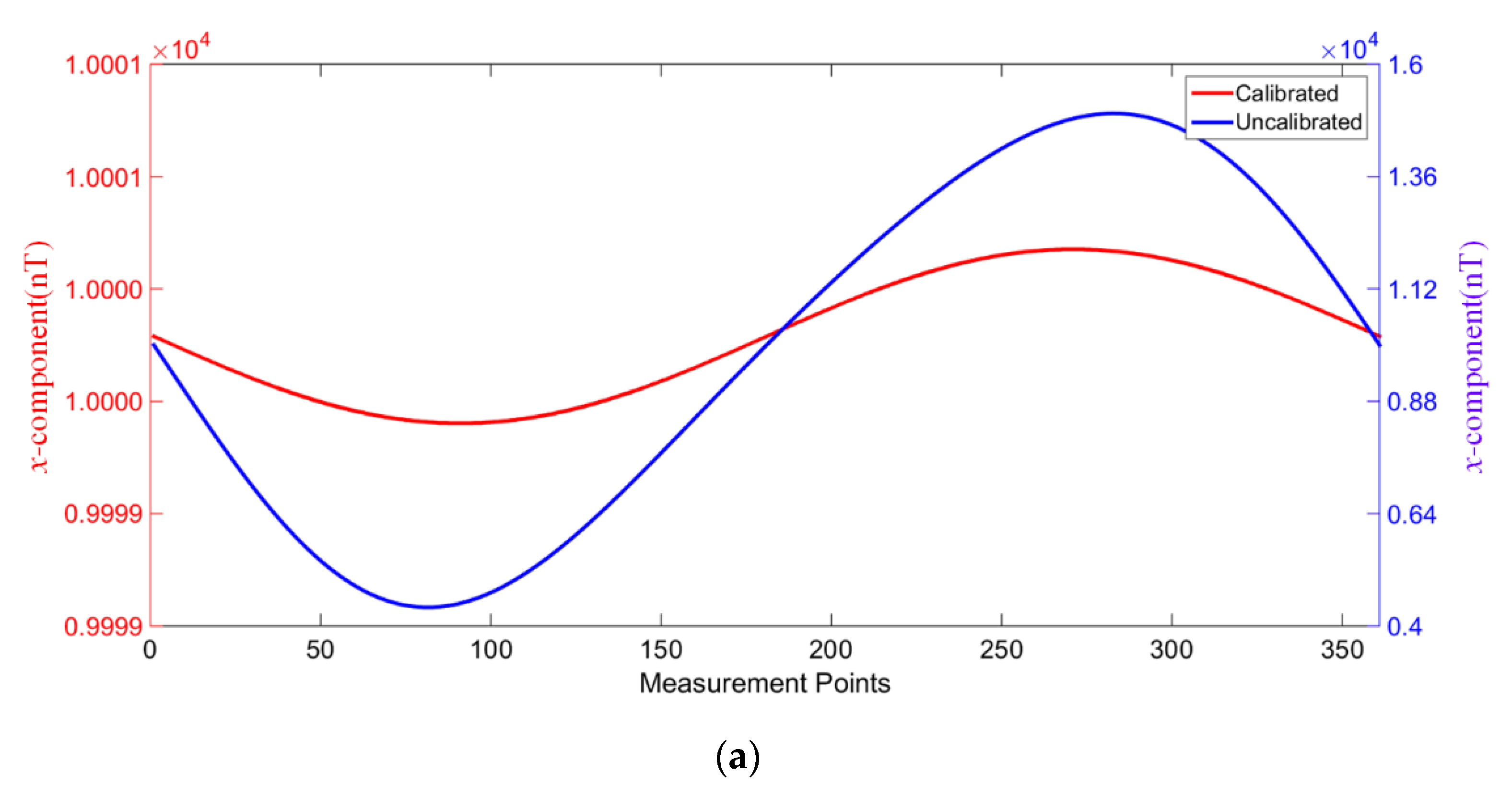
4.2. Simulation Results and Analysis

The calibration results are shown in Figure 5. After restoring the data to the geographic coordinate system, the deviation between the calibrated value and the preset value of the simulation experiment is shown in

Table 2. Calibration result of simulation experiment.

Parameter	Performance
x-component	≤0.5 nT
y-component	≤0.5 nT
z-component	≤0.5 nT

, which verifies the feasibility of this improved method. The virtual vector is set arbitrarily and has no relation with the preset background magnetic field value. Therefore, the simulation experiment shows this method is insensitive to the selection of the virtual vector.

5. Experiment

5.1. Setup of Experiment

The experimental system is composed of a tri-axis magnetometer, an INS, and a non-magnetic turntable, the performance specifications of which are shown in

Table 3. The performance specifications of INS and magnetometer.

Sensor	Feature		Value
Magnetometer (Bartington, Witney, UK)	Measurement range		±100,000 nT
	Accuracy		±0.1 nT
	Orthogonality error		<0.1°
	Scaling error		<±0.5°
	Offset error		<±5 nT
INS (NovAtel, Hexagon, SWE)	Accuracy (RMSE)	Heading	0.06°
		Pitch	0.015°
		Roll	0.015°

. The INS and magnetometer are fixed on the same carbon-fiber frame so that they can rotate synchronously. A diagram of the experimental system is shown in Figure 6. During the installation of these two sensors, the misalignment error is generated randomly. The performance of the proposed method in practical application is verified.

The experiment was conducted in an open space without magnetic interference. The local magnetic gradient is about 86 nT/m and the magnetic diurnal variation is less than 5 nT in one hour.

5.2. Experiment Results and Analysis

In the field experiment, the experimental data are obtained by rotating the three-component magnetic survey system about an arbitrary axis. The situation of experimental data trajectory before and after calibration can be seen in Figure 7. The attitude of the trajectory changes after calibration.

It is very difficult to obtain the standard values of the three-component magnetic field at the experimental site and the misalignment error calibration has no effect on the total field values measured by the magnetometer. The misalignment error of the magnetic survey system is finally reflected in the measurement results of the x, y and z components, that is, the misalignment error causes the fluctuation of the measurement values. Theoretically, under the condition of no misalignment error, the fluctuation of the magnetic measurement data after being restored to the geographical coordinate system is zero. Therefore, the calibrated magnetic measurement data can be restored to the geographic coordinate system and the effect of the misalignment error calibration of the magnetic survey system can be evaluated by the fluctuation of the three-component magnetic data.

The calibration results of the field experiment are shown in Figure 8. The fluctuation range, absolute deviation value, and standard deviation value are used to judge whether the method is effective in calibrating the misalignment error. Numerical values of these evaluation indicators are shown in

Table 4. Calibration results of the experiment data.

Parameter	Fluctuation Range (nT)		Absolute Deviation Value (nT)		Standard Deviation Value (nT)
	calibrated	uncalibrated	calibrated	uncalibrated	calibrated	uncalibrated
x component	20.991	1914.921	4.144	573.678	4.830	648.881
y component	33.105	3588.321	8.222	1187.153	9.267	1305.149
z component	23.936	1868.731	4.988	614.812	5.831	677.237

, which can reflect the dispersion degree of calibrated and uncalibrated data. By calculating the numerical ratio of these evaluation indicators, the improved method proposed in this paper reduces the fluctuation value of the x, y, z-component to 1.09%, 0.92%, 1.28%, respectively. The absolute deviation value is reduced to 0.72%, 0.70%, 0.81%, respectively. The standard deviation value is reduced to 0.74%, 0.71%, 0.86%, respectively. The calibration improves the dispersion degree of the experimental data significantly, which indicates that the misalignment error is effectively eliminated. The calibration results of the field experiment show that the proposed method has high operability and high precision in a practical application.

6. Conclusions

An improved method for calibrating the misalignment error is proposed in this paper. Firstly, the misalignment error is modeled. Then, we set a constraint to transform the calibration of misalignment error into estimating calibration parameters to minimize the value of the objective function. Finally, the MATLAB’s NLS function is used to estimate the calibration parameters. The feasibility and performance of the improved method are verified by simulation and the field experiment.

Compared to the preceding methods, this improved method has the following advantages: (1) The first advantage is that the method has high operability. Because the normal vector and tangent vector of data trajectory are used simultaneously, the calibration experiment only needs to rotate about an axis once and the axis of rotation can be arbitrarily chosen. In addition, the DPI method and Gao’s method cannot uniquely estimate the calibration matrix R with the same data. These two methods need at least two sets of dates rotated about different axes to calibrate the misalignment error. (2) The second advantage is that the method is insensitive to the selection of the virtual vector. The virtual vector can be arbitrarily chosen, and different virtual vectors do not affect the accuracy of calibration.

Future research should focus on developing a method to accurately fit data trajectories. The error of a non-magnetic turntable could lead to the data not in the same plane. The discretization of data could lead to a decrease in calibration accuracy.

References

1. Virgil, C.; Ehmann, S.; Hördt, A.; Leven, M.; Steveling, E. Reorientation of three-component borehole magnetic data. Geophys. Prospect. 2015, 63, 225–242. [Google Scholar] [CrossRef]
2. Sheinker, A.; Frumkis, L.; Ginzburg, B.; Salomonski, N.; Kaplan, B.Z. Magnetic Anomaly Detection Using a Three-Axis Magnetometer. IEEE Trans. Magn. 2009, 45, 160–167. [Google Scholar] [CrossRef]
3. Barczyk, M.; Lynch, A.F. Integration of a Triaxial Magnetometer into a Helicopter UAV GPS-Aided INS. IEEE Trans. Ind. Electron. 2012, 48, 2947–2960. [Google Scholar] [CrossRef]
4. Heekwon, N.O.; Kee, C. Enhancement of GPS/INS Navigation System Observability Using a Triaxial Magnetometer. Trans. Jpn. Soc. Aeronaut. Space Sci. 2019, 62, 125–136. [Google Scholar]
5. Mu, Y.; Wang, C.; Zhang, X.; Xie, W. A Novel Calibration Method for Magnetometer Array in Nonuniform Background Field. IEEE Trans. Ind. Electron. 2019, 68, 3677–3685. [Google Scholar] [CrossRef]
6. Bernalpolo, P.; Martinezbarbera, H. Temperature-Dependent Calibration of Triaxial Sensors: Algorithm, Prototype, and Some Results. IEEE Sens. J. 2020, 20, 876–884. [Google Scholar] [CrossRef]
7. Pan, D.; Li, J.; Jin, C.; Liu, T.; Lin, S.; Li, L. A New Calibration Method for Triaxial Fluxgate Magnetometer Based on Magnetic Shielding Room. IEEE Trans. Ind. Electron. 2020, 67, 4183–4192. [Google Scholar] [CrossRef]
8. Ghasemimoghadam, S.; Homaeinezhad, M.R. Attitude determination by combining arrays of MEMS accelerometers, gyros, and magnetometers via quaternion-based complementary filter. Int. J. Numer. Model. Electron. Netw. Device Field 2018, 31, e2282. [Google Scholar] [CrossRef]
9. Liu, Z.; Wang, L.; Li, K.; Han, H. Analysis and improvement of attitude output accuracy in tri-axis rotational inertial navigation system. IEEE Sens. 2020, 20, 6091–6100. [Google Scholar] [CrossRef]
10. Yue, Z.; Lian, B.; Tang, C.; Tong, K. A novel adaptive federated filter for GNSS/INS/VO integrated navigation system. Meas. Sci. Technol. 2020, 31, 085102. [Google Scholar] [CrossRef]
11. Primdahl, F. Astrid-2 magnetometer and star sensor intercalibration. Magnetic Observatory 15–16 May 1997. Exp. Biol. Med. 1997, 58, 205–209. [Google Scholar]
12. Pang, H.; Zhu, X.; Pan, M.; Zhang, Q.; Wan, C.; Luo, S.; Chen, D.; Chen, J.; Li, J.; Lv, Y. Misalignment calibration of geomagnetic vector measurement system using parallelepiped frame rotation method. J. Magn. Magn. Mater. 2016, 419, 309–316. [Google Scholar] [CrossRef]
13. Li, X.; Li, Z. A new Calibration Method for Triaxial Field Sensors in Strap-down Navigation systems. Meas. Sci. Technol. 2012, 23, 105105. [Google Scholar] [CrossRef]
14. Zhu, X.; Zhao, T.; Cheng, D.; Zhou, Z. A three-step calibration method for tri-axial field sensors in a 3D magnetic digital compass. Meas. Sci. Technol. 2017, 28, 055106. [Google Scholar] [CrossRef]
15. Fang, J.; Sun, H.; Cao, J.; Zhang, X.; Tao, Y. A Novel Calibration Method of Magnetic Compass Based on Ellipsoid Fitting. IEEE Trans. Instrum. Meas. 2011, 60, 2053–2061. [Google Scholar] [CrossRef]
16. Fang, J.; Sun, H.; Cao, J.; Zhang, X.; Tao, Y. A Calibration Method for the Misalignment Error between Inertial Navigation System and Tri-Axial Magnetometer in Three-Component Magnetic Measurement System. IEEE Sens. J. 2019, 19, 12217–12223. [Google Scholar]
17. Cheng, H.; Gupta, K.C. An Historical Note on Finite Rotations. J. Appl. Mech. 1989, 56, 139–145. [Google Scholar] [CrossRef]
18. Baritzhack, I.Y. Extension of Euler’s theorem to n-dimensional spaces. IEEE Trans. Aerosp. Electron. Syst. 1989, 25, 903–909. [Google Scholar]
19. Paielli, R.A. Global transformation of rotation matrices to Euler parameters. J. Guid. Control Dyn. 1992, 15, 1309–1311. [Google Scholar] [CrossRef]
Figure 1. The diagram of misalignment error between a magnetometer and an inertial navigation system (INS).
Applsci 10 06707 g001
Figure 2. The diagram of Euler’s rotation.
Applsci 10 06707 g002
Figure 3. The diagram of measured data.
Applsci 10 06707 g003
Figure 4. The diagrams of measured data and auxiliary data.
Applsci 10 06707 g004
Figure 5. The calibration results. (a) The x component; (b) The y component; (c) The z component.
Applsci 10 06707 g005aApplsci 10 06707 g005b
Figure 6. Diagram of experimental system.
Applsci 10 06707 g006
Figure 7. Trajectory coincidence after calibration.
Applsci 10 06707 g007
Figure 8. The calibration results. (a) The x component; (b) The y component; (c) The z component.
Applsci 10 06707 g008aApplsci 10 06707 g008b