1. Introduction
Volcanoes represent a significant threat and, at the same time, are a huge attraction since antiquity for populations living nearby due to their fertile lands. At present, large populations live near active or quiescent volcanoes and thus are at risk of their possible eruptions. It is well known that volcanic eruptions can determine increasing air pollution levels; furthermore, they can influence climate [
1] and, in some circumstances, produce lethal eruptions that destroy the surrounding environment and cause serious losses to national/international economies. Cautious valuation of volcano comportment and activity state is required to mitigate these effects, which can be carried out by instruments dedicated to volcanic control [
2].
Volcanologists can nowadays infer in real time, by modern technological and modeling developments, the signals coming from seismic and ground deformations that usually happen before eruptions. It is possible to know of an imminent eruption by detecting the stress changes and magma accumulation/flow, thanks to the improvements in broadband seismometers, models, and tools for processing seismic signals [
3], and the constant implementation of satellite-based (GPS, Global Positioning System [
4] and InSAR, Interferometric Synthetic Aperture Radar [
5]) geodetic observations [
6].
Volcanic plumes, fumaroles, and degassing grounds release incessantly magmatic volatiles (e.g., H
2O, SO
2, and CO
2) [
7], representing the external appearance of deep magma degassing [
8,
9]. These volatiles are a source of priceless data for forecasting the likelihood of a volcanic eruption. Therefore, accurate knowledge of volcanic gas composition and flux can provide alerts on possible eruptions [
10], and provide insights into the geophysical processes occurring in the inner parts of volcanoes.
As far as abundancy is concerned, CO
2 is the second gas in volcanic fluids. Unfortunately, in contrast to SO
2, its measurements are much more complicated. In fact, efforts to achieve standoff detection of the volcanic CO
2 flux have been discouraged by technical challenges. This is mainly due to the large atmospheric background, about 400 parts per million (ppm), which makes it difficult to resolve the volcanic CO
2 signal. For these reasons, there are few volcanic CO
2 flux data in geophysical studies (see [
11,
12,
13,
14] for fresh research).
In fact, SO
2 can be found at the parts per billion concentration in the unperturbed atmosphere, therefore its volcanic flux can be detected via routinely collected data from the ground (e.g., DOAS, Differential Optical Absorption Spectroscopy [
15]) and in space using UV (Ultraviolet) spectroscopy [
16,
17,
18]. Instead, standoff detection of volcanic CO
2 has only been accomplished during eruptions of mafic volcanoes, where ground-based Fourier transform infra-red (FTIR) spectrometers can take advantage of magma/hot rocks as efficient light sources [
19]. Conversely, monitoring of the far more usual “passive” CO
2 releases from quiescent volcanoes has implied access to risky summit craters for direct measurement of fumaroles [
20] or in situ sampling of plumes by implementing Multi-GAS (Multi-component Gas Analyzer) systems [
21] or Active-FTIR [
22].
The employment of modern systems and networks for volcanic gas observations [
8,
20,
23] has made it possible to make significant progress in direct sampling techniques for volcano monitoring. This has resulted in an improvement in time resolution of traditional ground-based volcanic gas observations [
24]. Moreover, taking advantage of fast advancements in optoelectronics, especially in the last two decades including new coherent sources, detection systems, and spectrometric devices, we have at present many optical remote techniques, both passive and active, ground-based, airborne, and even space-borne, that are applicable to issues involving Earth CO
2 degassing [
12,
14]. The improvements of volcanic gas measurements in terms of numbers, quality, and time duration are providing evidence that CO
2 is the gas most directly linked to “pre-eruptive” degassing processes [
21]. As confirmation of this fact, precursory increases in CO
2 plume flux have been recently detected at several volcanoes [
25] such as at Mt. Etna, the most active and dangerous volcano in Europe [
26].
Taking into account the potentialities given by data on the volcanic CO2 flux for predicting eruptions, the ability to remotely monitor this flux with a high time resolution is an important step ahead in current volcanology.
Considering the stringent requirements of volcanological research and the great advantages of active optical remote sensing (e.g., measurement not dependent of sunlight or other radiation sources, safe monitoring distance, probing of sites difficult to access, large areal coverage, higher accuracy than passive techniques, etc. [
14]), ground-based lidar systems have represented, since their creation, a valuable option for the remote detection of volcanic gases and aerosols. Such systems share many advantages with seismic and deformation monitoring with respect to direct sampling; in a nutshell, they can perform measurements from a safe area, while also allowing (semi)-continuous operation during eruptions. Moreover, gas amounts can be retrieved non-invasively in near real-time, obviating the need for successive laboratory analysis, thus avoiding possible sample contamination, and—unlike in situ sampling—standoff sensing techniques measure integrated or range-resolved gas concentrations through cross-sections of the plume, thus providing a more informative characterization of composition and flux of the volcanic plume [
8].
Lidar systems have increasingly been used since the early 1980s for the valuation of volcanic hazards (e.g., during the Soufriere and Mt. St. Helens eruptions in 1979 and 1981, respectively) [
8]. Over the last 30 years, several lidars have been deployed to obtain data on the concentrations and fluxes of sulfate aerosol [
27,
28,
29] and ash [
30]. Furthermore, laser remote sensing systems have been used to detect volcanic particles in the troposphere at Mt. Etna (Italy) [
31] and in the lower stratosphere during the Pinatubo eruption (Philippines) [
32]. In particular, the lidar at Garmisch-Partenkirchen was one of the first examples of volcanic lidar implemented to observe the spread of the stratospheric volcanic plume (from 10 to 28 km) by evaluating the time-series of vertical profiles of the scattering ratio and vertically integrated column of the backscatter coefficient using a Nd:YAG laser operating at 532 nm. These measures were affected by the following average errors: peak scattering ratio: ±4–5% and integrated backscatter coefficient: ±10% [
32].
DIAL-Lidar (Differential Absorption Light Detection and Ranging), or simply DIAL, is based on the fast switching of the wavelength of laser pulses on- and off-absorption of the molecule under study. From the application of the Beer–Lambert law to the ratio of the lidar signals (detected radiation vs. range) retrieved at both wavelengths, the range-resolved molecule concentrations (ppm) can be obtained, thus determining the two-dimensional or even three-dimensional plume morphology. This achievement is beyond the capabilities of FTIR, COSPEC (Correlation Spectrometer), and DOAS [
15], which provide the path length integrated concentrations (ppm m). DIAL has been deployed at the main Italian volcanoes with UV lasers for tracking the total fluxes of SO
2 [
28,
33]. In particular, the first example of the quantification of volcanic SO
2 fluxes by using the DIAL (active) technique is reported in [
33] where it was extensively compared with passive monitoring techniques (DOAS and COSPEC). In the previously mentioned work, the lidar-based SO
2 fluxes were 50% higher on average than those derived with other standard passive techniques (COSPEC and DOAS) commonly used in volcanology. This mismatch was interpreted as evidence of possible scattering-induced errors in the passive techniques.
More recently, ATLAS (Agile Tuner Lidar for Atmospheric Sensing), a ground-based DIAL system, has been implemented to perform measurements of water vapor flux at the Stromboli volcano (Italy) [
34]. To our knowledge, this was the first time that lidar retrieved water vapor concentrations in a volcanic plume.
Finally, the Cloud-Aerosol Lidar with Orthogonal Polarization (CALIOP), an elastic backscatter lidar operated from a satellite, was used to observe volcanic ashes from 15 to 20 April 2010, just after the explosion of the Eyjafjallajökull volcano (Iceland) [
35]. This has opened up new scenarios in future volcanic-lidar applications.
However, the apparatuses previously described were costly, heavy, and not effective enough to be implemented in the long-term period. Even though DIAL provides unprecedented opportunities to volcanologists, it requires more advancement to become a reliable technique for routine observations.
In order to fill these gaps, a new DIAL system, designed to measure the volcanic CO
2 flux, was developed as part of the ERC (European Research Council) Starting Grant Project “BRIDGE”. The BrIdge voLcanic LIdar (BILLI), assembled at the ENEA (Italian National Agency for New Technologies, Energy and Sustainable Economic Development) Research Center of Frascati by the FSN-TECFIS-DIM group (Diagnostics and Metrology Laboratory) [
36], successfully retrieved three-dimensional tomographies of volcanic CO
2 concentration in the plumes at Italy’s most hazardous volcanic areas: Pozzuoli Solfatara (Naples, Italy) [
21,
37,
38], the Stromboli volcano (Aeolians Islands, Italy) [
39,
40], and Mt. Etna (near Catania, Italy) [
41,
42].
As far as we know, lidar measurements of CO
2 have been performed in volcanic plumes only in recent times, due to the previously mentioned technical challenges and the extreme environmental operating conditions [
14,
21,
37,
38,
39,
40,
41,
42]. In the last decade, promising results have been obtained by using a variant of DIAL, known as the Integrated Path DIAL (IPDIAL), but mainly to monitor ambient CO
2 concentrations (e.g., power plants/industrial emissions), and an Open-Path laser Spectrometer (OPS) to measure volcanic CO
2 concentration and flux. However, despite the efforts to provide a remedy to some drawbacks of DIAL-Lidar systems (in terms of costs, complexity of the setup and maintenance, portability and integration time), the aforementioned systems had severe limitations such as the need of a topographic target to perform the measurements of CO
2, which were not range-resolved (only path averaged gas concentrations were retrieved). In addition, the volcanic CO
2 flux computed by OPS was affected by a large uncertainty [
14]. Therefore, it can be concluded that BILLI was the first range-resolved DIAL system used to remotely measure both CO
2 concentration and flux in a volcanic plume.
In particular, as will be shown in the following paragraphs, BILLI has been deployed to retrieve range-resolved profiling in wide plumes, thus providing spatio-temporal dispersion concentration maps and high-resolution CO
2 flux time-series. It has opened unprecedented possibilities in measuring volcanic CO
2: BILLI made it possible to clearly detect an excess of a few tens of ppm over a distance of more than 4 km, considering a spatial and temporal resolution of 5 m and 10 s, respectively [
42].
Quantifying the CO
2 output from Pozzuoli Solfatara (October 2014) [
21,
37,
38] and Stromboli (June 2015) [
39,
40,
41] allows for the interpretation, and if possible, the forecast, of the upcoming development of the volcano scenario, with huge benefits to the population living nearby. These examples show the huge social values of lidar systems in monitoring gas emissions. Moreover, observations at densely populated volcanic regions will have a high societal impact throughout Europe. In this regard, the potential of our system has also been confirmed by the results acquired during the last experimental campaign, carried out between July and August 2016 at Mt. Etna [
42], retrieving a plume peak beyond 4 km.
The main goal of these experimental campaigns was to measure the exceedance of in-plume CO2 concentration and flux to provide useful information to volcanological research for a precocious alert to the population in the event of eruptions.
In this paper, after a description of BILLI, special emphasis will be given to data processing and analysis of the experimental results, which will be thoroughly discussed. This was made possible by means of automatic software procedures written in MATLAB and based on the newly designed BRIDGE DIAL data processing technique. Significant CO2 concentration profiles, dispersion maps, and time-series of CO2 flux will be shown. Moreover, our monitoring was assessed by conventional data and local meteorological measurements.
Finally, thanks to the BILLI system and from a complete time-resolved plume evolution, it was also possible to retrieve the wind velocity (Stromboli field campaign, 2015), a useful parameter for the CO2 flux calculation and for the mitigation of volcanic hazards, especially in the field of air traffic security.
3. Results and Discussion
A brief overview of the experimental campaigns carried out over three years by the BILLI system will be presented and discussed here.
The first experimental campaign was carried out during October 2014. The system was placed ≈100 m far from the fumaroles of Pozzuoli Solfatara (Pisciarelli, Phlegraen Fields). The system performed a horizontal scan at different elevations, retrieving, for the first time, CO
2 concentration dispersion maps and time-series of lidar-derived CO
2 fluxes [
21,
37,
38].
About ten months later (June, 2015), other tests were carried out at Stromboli Volcano Island, where BILLI operated nearly 24 h for almost a week, performing horizontal and vertical scans. CO
2 excess of a few tens of ppm was measured in some minutes in the volcanic plume up to a distance of nearly 3 km far from the system. In addition, in this case, daily cycles of CO
2 flux were successfully retrieved [
39,
40,
41].
Finally, the potential of the BILLI DIAL system was confirmed by the last field campaign at Mt. Etna at the end of July 2016, where, for the first time, in-plume CO
2 concentration peaks were retrieved at a distance exceeding 4 km [
42].
It should be noted that during all field campaigns, eye safety regulations were followed and weather did not alter the BILLI operation, except for a moderate influence of the wind, as is reported in
Section 3.2 [
21,
37,
38,
39,
40,
41,
42].
3.1. The Experimental Campaign of Pozzuoli Solfatara
The first field experiment was conducted at the Phlegraen Fields volcano [
21,
37,
38]; this is a rising caldera including Pozzuoli and the suburbs of Naples, among the most inhabited zones of Italy. The bradyseismic crises of the volcano produced thousands of shallow earthquakes, and its activity has been often, even if not continuously, active in the last few decades. Scientists and stakeholders observed these recent crises, despite them not evolving into an eruption, bearing in mind the related important hazard mitigation problems and the linked necessary interventions. These issues have become even more critical taking into account that ground uplift restarted in 2012, with the intensification of degassing activity, in the caldera center and at the main surface hydrothermal manifestations of Solfatara and Pisciarelli. Current uplift/degassing unrests observed in Pozzuoli are probably due to intermittent injections of carbon dioxide-rich gas in the hydrothermal system of the volcano, indicating that fresh magma is supporting a strong inflow of gas from deep layers. Here, attention has been focused on the degassing fumarolic vent of Pisciarelli that, besides a small augmentation in discharge temperature (from less than 95 °C up to 110 °C), has visibly escalated in degassing activity over the past decade (the carbon dioxide concentration in fumaroles has also risen), making it the most active among the Italian fumarolic vent areas. Therefore, quantifying the CO
2 output from Pisciarelli is vital for the interpretation and possibly the prediction of future changes in this volcanic zone [
21].
The system measured nearly continuously during both 15 and 16 October 2014, after the experimental setup on 14 October. During the measurement operations, BILLI performed a horizontal scan of the almost vertical plume in the 198°–232° range of azimuth angles (see
Figure 3a). The elevation of 12° was used mostly for the performed scans, where the plume structure was fully resolved and the lidar echoes were more intense. Controls proved that at lower and higher elevations, the plume was often either optically too thick or too spread, so only a few additional scans at 0°, 6°, and 15° were completed. A total of 200 lidar returns (100 at λ
ON and 100 at λ
OFF, see
Table 2) were ascribed to a single profile and averaged to improve the SNR; in this way, the sampling frequency of the lidar echoes was 0.05 Hz, which corresponded to a 20-s time resolution. As already discussed, the space resolution of BILLI was 5 m. The combination of about 25 profiles yielded a total scan of the plume in around 10 min [
21,
37,
38].
Thanks to the BRIDGE DIAL technique (see
Section 2.2) it was possible to retrieve, globally, up to 40 scans of CO
2 concentration in excess in the plume and, at the same time, the CO
2 flux time-series. The whole dataset covered almost three days of operation, for a maximum of nine consecutive hours. Examples of the CO
2 dispersion map and flux time-series are reported in
Figure 3a,b, respectively [
21].
Figure 3a illustrates the results of a typical scan (using the polar diagram) through the plume. When the laser beam intercepted the plume, peak CO
2 concentrations of up to 5000 ppm were measured. The plume was typically crossed at azimuth angles of 205–225° and at distances in the range of 50–70 m from the system. At azimuth angles <205° and >225°, or at distances <50 and >70 m, BILLI retrieved the carbon dioxide concentration usually found in ambient air, thus providing confirmation that the laser beam was able to scan the whole plume. This result directly corresponded to the most vigorously degassing fumarolic vent of Pisciarelli. An evident CO
2 peak, in scans performed at an elevation angle of 6°, was even clearer in the same fumarolic vent. This fact was also due to the reflection of the laser beam off the rockfaces enclosing the vent [
21,
37,
38].
Figure 3b, instead, illustrates CO
2 flux time-series from the fumarolic system. Here, the cross-correlation analysis, applied to sequences of visible images of the moving plume that were co-acquired at a high rate (30 Hz) by a digital optical camera, was applied to achieve the vertical plume transport velocity. The overall error in the calculated plume velocity was in the range from 10 to 28%, leading to a total error of CO
2 fluxes from 15 to 33% [
21].
Thanks to the high time resolution (around 10 min) of the system, it was possible to follow important intraday dynamics, nearly impossible to measure with conventional instruments for several reasons such as environmental difficulties, high costs, instrumentation ineffectiveness, and the larger amount of ambient air carbon dioxide that is present along the line of sight between the spectrometer, target (plume), and the source of photons (sun, magma, and lava fragments).
The strong changes over timescales of tens of minutes are clear in the Pisciarelli hydrothermal site such as from a peak emission of 4.4 Kg/s (at 18:23 h local civil time on 15 October) down to 1.9 Kg/s after about 60 min. Apart from these fast variations, our data indicate a general constancy of CO
2 output over timescales of a few days. The mean carbon dioxide emissions for 15 and 16 October 2014 were quite similar (2.63 ± 0.98 and 2.52 ± 0.84 Kg/s), corresponding to the total daily outputs of 256 ± 89 and 218 ± 71 tons, in that order. Furthermore, the carbon dioxide fluxes measured by BILLI were in overall agreement with other estimations carried out with in situ data obtained with a portable gas analyzer [
21].
Nevertheless, our system has the following advantages: (i) external light sources are not required; (ii) measurements can be performed without risk from a remote area; (iii) the spatio-temporal resolution is finer; and (iv) the morphology of the plume can be obtained in some minutes.
Moreover, the big difference between the lidar echoes coming from the plume and ambient air allows the operator to disentangle the carbon dioxide of volcanic origin, and therefore to quantify the volcanic carbon dioxide flux. Such measurements are new in geophysics, and promise to contribute to volcanological research.
Even though, at this experimental stage, a considerable number of further developments are needed (e.g., system miniaturization, automation, independent measurements of in-plume wind velocity, and long-distance remote sensing), the system performed the first measure of CO
2 concentration and flux in a volcanic plume [
21].
3.2. The Experimental Campaign of Stromboli Volcano
The second field experiment was conducted at Stromboli Volcano Island. The volcanic activity on the island is generally considered “regular” and mild (strombolian). Larger-scale vulcanian-style explosions occasionally occur. Although these events, locally referred to as “major explosions” or “paroxysms”, are not frequent and are short-lived (from tens of seconds to a few minutes), they could be extremely dangerous for locals and authorized personnel, since they produce fallout of coarse pyroclastic materials over wide dispersal areas. Moreover, neither geophysical nor volcanological precursor signals were observed before these events occurred. This could be due to the fact that they originate deep in the crustal roots of the volcano plumbing system. However, it has been observed that the previously cited events are systematically preceded by days/weeks of anomalous CO
2-rich gas leakage from the Stromboli’s deep (8–10 km) magma storage zone. For these reasons, volcanologists are considering with increasing interest CO
2 flux emissions from the open-vent crater plume for the monitoring of volcanic activity and hence for the assessment and mitigation of the related hazards [
41].
As in other volcanic areas, at Stromboli, the volcanic gas CO
2 from a combination of simultaneously measured SO
2 fluxes and plume CO
2/SO
2 ratios has also been recently evaluated [
7,
11]. Even though the remote measure of SO
2 flux is possible by implementing UV spectroscopy [
16], the CO
2/SO
2 ratio requires in situ direct sampling/measurements close to hazardous active vents. For the previous reasons, the implementation of the BILLI DIAL system for the remote observation of the volcanic CO
2 flux, from distant and less risky locations, is a real advantage.
The system operated almost continuously from 24 to 29 June 2015 despite the harsh environmental conditions due to the presence of high humidity, acid vapors, and re-suspended dust. It was placed inside the fence of the local ENEL (main Italian electric company) power plant in the Scari area, ≈2.5 km from the degassing vents on the volcano summit, between the margins of morphological peaks known as Pizzo and Vancori, 918 and 924 m, respectively, above sea level (ASL). The laser beam typically scanned the azimuth angles from 235.3° to 253.6° and the elevation angles from 15.2° to 27.4°.
As stated in
Section 2.1, in order to reduce the differential absorption cross section of CO
2, the transmitted wavelengths were changed with respect to the previous campaign (see
Table 2). As a result, longer distances were reached by the laser beam. Furthermore, the implementation of a photo-acoustic cell filled with pure CO
2 allowed us to reduce the systematic uncertainty, dominated by instability in wavelength setting, to 5.5% (see
Section 2.2.5). Compared to the previous experimental campaign, the pulse repetition rate remained unchanged (10 Hz), instead both the temporal resolution was slightly modified and set at 10 s because only 100 lidar returns (50 at λ
ON and 50 at λ
OFF, interlaced) were averaged for each scan to increase the SNR. A further improvement of the SNR and, therefore, of the accuracy of both CO
2 concentration and flux measurements was possible by employing filtering algorithms and curve fitting techniques, in the preliminary data analysis steps (see
Section 2.2.1). Furthermore, by combining about 50 profiles, it was possible to obtain both vertical and horizontal plume scans in less than 10 min. Eventually, by processing several repeated scans (usually 10) acquired at different elevations, we also retrieved three-dimensional tomographies of the volcanic plume [
39,
40,
41].
Thanks to an improved and fully automated version of the BRIDGE DIAL data processing routine (taking into account local conditions and the changes in system setup), it was possible to retrieve up to 180 scans of CO
2 concentration in excess in the plume and, at the same time, the CO
2 flux time-series. In addition, thanks to a further data processing routine (see
Section 2.2.3), it was possible to estimate the plume transport velocity and, hence, the local wind velocity. The whole dataset covered almost six days of operation, for a maximum of 12 consecutive hours. Examples of CO
2 dispersion map, wind profiles, and flux time-series are reported in
Figure 4a,b, respectively [
39,
40,
41].
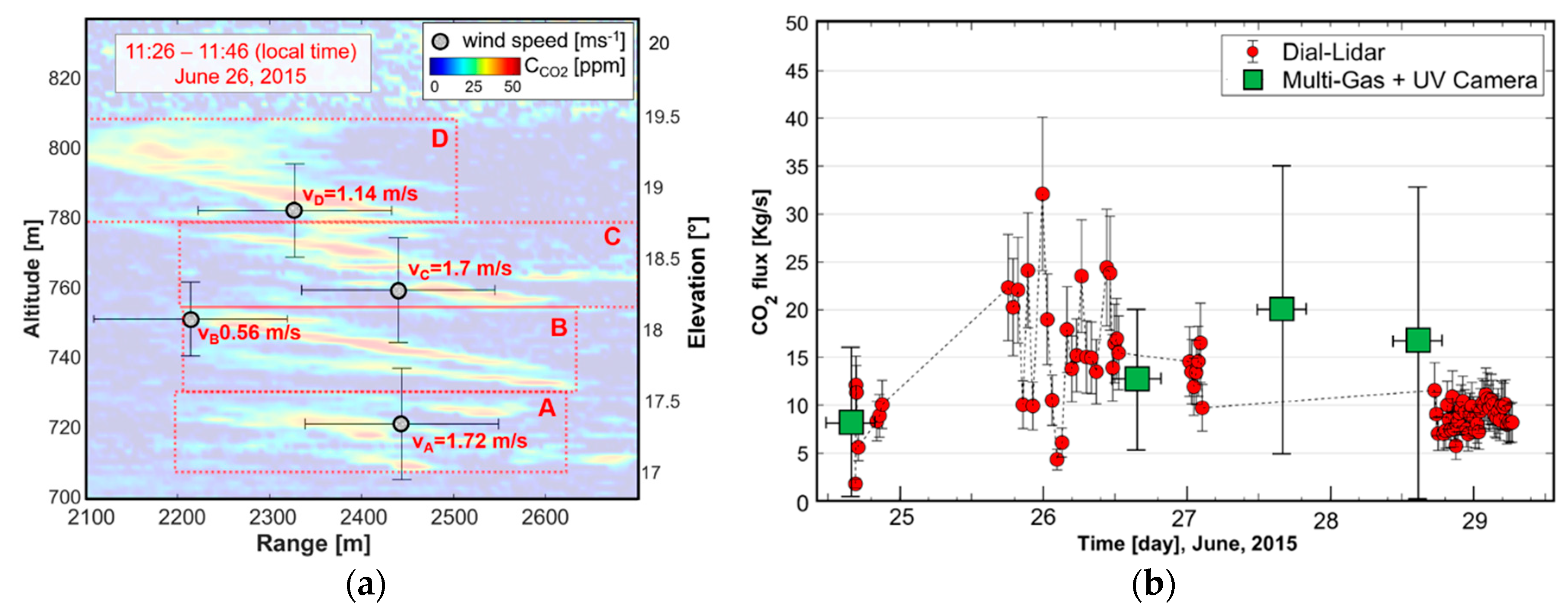
Figure 4a illustrates the results of a typical vertical scan through the plume as a function of range (X axis), elevation angle, and altitude (Y axes). The tomography reported above was extrapolated from the measurement session performed on 26 June 2015 between 11:26 and 11:46 (local civil time), and it represents a dataset acquired as a single group of measurements slowly stepping up in elevation angle (from 16.8° to 20°) over the course of about 20 min, since, during that time, the plume displacement was extremely clear. The carbon dioxide concentration in the zone under study is indicated by the color scale, with peaks exceeding 60 ppm. Here, the volcanic plume was encountered in the 2150−2600 m range, from 17 to 19.5° elevation angles, and a fixed azimuth of 237.8°. Regions highlighted with red boxes and named as A, B, C, and D were posited to be the same set of scatterers being tracked over time. Therefore, they represent a useful example for summarizing the time evolution of inhomogeneities relative to the volcanic plume. To appreciate these displacements, it is necessary to specify that particles detected in region A need a certain amount of time to move to the regions B (about 3 min), C (about 6 min), and D (about 9 min). As observed in the field, these movements were mainly due to the presence of wind blowing from north–northwest [
40].
Considering both vertical and horizontal scans of the whole campaign, the beam hit the plume at azimuth angles in the range 237–251°, elevation angles in the range 16.5–20° (which means altitude of 700–830 m) and at distances in the range 2200–2500 m. For azimuth angles <237° and >251°, or for distances <2200 and >2500 m, BILLI retrieved the carbon dioxide concentration we usually find in ambient air, thus providing confirmation that the laser beam was able to scan the whole plume. This result was confirmed by direct observations [
37,
39].
The quality of the results (as in the example shown in
Figure 4a), combined with the high temporal resolution of the acquired data, allowed us to perform, almost simultaneously with in-plume CO
2 concentrations, the first independent measurement of plume transport velocity (v
p) and therefore of the wind velocity, using the correlation method mentioned in
Section 2.2.3 and detailed in a previous work [
40]. As already mentioned, the assessment of the wind velocity could be crucial for both the CO
2 flux retrieval and air traffic control applications. In this regard, a set of data (lasting about 90 min) was selected from the morning of 26 June 2015.
An example of vertical wind profile was superimposed on the same dataset (lasting about 20 min) of the CO
2 concentration dispersion map reported in
Figure 4a, showing a high consistency with the time evolution of the in-plume spatial aerosol inhomogeneities (see the previously mentioned A, B, C, D regions highlighted with red boxes).
The global weighted average value of wind velocity was found equal to 1.1 ± 0.4 m/s for the whole measurement test session. Although promising in terms of cost saving and speed, our measurements were slightly different from the ones acquired by the UV camera [
41] and affected by a high uncertainty level due to the presence of wind blowing in the perpendicular direction, with respect to the system location, the worst observing condition for the tracking of the wind [
40]. Nonetheless, they were found in agreement, within the error bar, with weather data acquired by conventional devices and with a precision comparable to that of stand-alone fixed-beam correlation lidars. It should be noted that, a comprehensive comparison with local data was considered unreliable, since the nearest weather station on the island performed 6-h average of weather parameters acquired at 4 m ASL and not at the same height of the laser beam pointing. For these reasons, efforts will have to be devoted to advance the configuration of BILLI (e.g., implementing at least three beams or a 360-degree scanning mirror) to fully and accurately retrieve the three components (x, y, and z) of the wind velocity [
40]. Therefore, due to the constraints (in terms of dataset duration and results reliability) of our preliminary tests on the fast tracking of wind velocity, during the Stromboli campaign, CO
2 flux time-series were retrieved using v
p values obtained from processing the sequences of UV camera images [
41].
Once having obtained the CO
2 dispersion maps and the plume transport velocity using the method described in
Section 2.2.4, it was possible to retrieve the CO
2 flux time-series with a cumulative uncertainty equal to 25% (dominated by the integration area uncertainty), as reported in
Figure 4b [
41]. The results confined the CO
2 flux during 24–29 June 2015 in the range from 1.8 ± 0.5 to 32.1 ± 8.0 Kg/s. The daily mean values of CO
2 flux were obtained by averaging all successful results for each measurement day. The values range from 8.3 ± 2.1 (24 June) to 18.1 ± 4.5 (25 June) Kg/s and corresponded to daily emissions of 718 and 1565 tons, in that order. These data are in agreement with past carbon dioxide estimates carried out at Stromboli. Moreover, in
Figure 4b, our lidar-based CO
2 fluxes were compared with alternative measurements, obtained by multiplying the CO
2/SO
2 ratio by the SO
2 flux, which is obtained using the traditional Multi-GAS + UV spectroscopy-based techniques. Despite the issues of the Multi-GAS + SO
2 flux approach reported in the literature (distinct temporal resolutions, and poor temporal alignment [
41]), we found a general agreement between the CO
2 fluxes obtained by BILLI and the usual instruments. This provided reciprocal trust for both techniques. Furthermore, BILLI-based carbon dioxide fluxes showed a better temporal resolution (≈16–33 min) and greater continuity. Moreover, BILLI as well as other standoff instruments, is intrinsically safe for operators [
41].
In conclusion, although several improvements were made (higher distances reached, fully automated operational routines, independent measurements of plume transport velocity) with respect to the previous campaigns [
39,
40,
41], efforts were needed to improve the system (in particular, improving portability and reducing power requirements). At the same time, further in-field tests were still necessary to fully explore the potential of our system, validating the reliability and efficiency of the data analysis method.
3.3. The Experimental Campaign of Mt. Etna
The last experimental campaign was carried out at Mt. Etna Volcano (3329 m ASL), a hostile and only partially inhabited region located near Catania, in Sicily. Mt. Etna is the largest and most important volcano in Italy and one of the most active volcanoes in the world. For these reasons, it was the ideal place to test our system performances [
42]. Similar to previous campaigns, the main goal was to measure the exceedance of in-plume CO
2 concentration and flux to provide useful information to volcanological research for a precocious alert to the population in the case of eruptions.
The area chosen for our experiments was the northeast summit crater of the volcano (other craters were discarded due to fact that volcanic plume is too dilute or only partially visible) and is characterized by extremes of temperature, high humidity, and rates of rainfall, and the presence of acid vapors, re-suspended dust and particles, which are toxic for humans and dangerous to the instrumentation. Notwithstanding the harsh environment, BILLI operated practically continuously for nearly a week (from 28 July to 1 August 2016 including an initial instrumental setup phase). During our experiment, the system was placed on a trailer, loaded on a truck, positioned into the courtyard of the INGV (Italian National Institute of Geophysics and Volcanology)observatory “Pizzi Deneri” at 2823 m ASL, on the northeast side of the main crater. This fixed position, about 500 m below the volcano summit, was ≈3 km far from the most important craters [
42]. Changing the elevation angle in the range 7–14° while fixing the azimuth angle (230°), BILLI vertically scanned the plume. Atmospheric profiles were recorded every 10 s, whereas each scan, obtained combining 24 profiles, was completed in ~15 min.
Taking into account the local conditions, both the setup (e.g., ON/OFF wavelengths) of the system and the data processing routine remained the same as the previous campaign, with the only exception of a reduction in the system weight (thanks to a rearrangement of the mechanical frame of the system). For these reasons, in this case, laser beam also reached longer ranges and the systematic uncertainty remained stable at 5.5%, whereas, as reported in the literature [
39], the statistical uncertainty of lidar profiles increased with range. At 2.5 km, a mean range, it was about 2% [
41,
42], while it exceeded 5% at 4.2 km [
42]. Thanks to the measures already adopted in the previous campaign and reported in
Section 2.1, the field setup at Mt. Etna, and the good weather conditions, a slight improvement in the system performances was observed.
Thanks to the BRIDGE DIAL technique, it was possible to retrieve up to 220 scans (lasting 10–20 min) of CO
2 concentration in excess in the plume and, at the same time, the CO
2 flux time-series. The whole dataset covered six days of operation, for a maximum of 12 consecutive hours. Examples of CO
2 profiles, dispersion maps, and flux time-series are reported in
Figure 5a–c, in that order [
40].
During the campaign, several configurations of plume were recognized, which varied as a function of acquisition time. In fact, both the magnitude and the size of the CO
2 plume were subject to change with the elevation of the laser beam pointing angle and, obviously, they were also influenced by the presence of wind [
42].
In general, for elevation angle values comprised within 7° and 9°, it was quite common to detect narrow plume peaks (extending for about 500 m with magnitude values not exceeding 140 ppm) attached or strictly close to the first or the second rockface of Mt. Etna. In fact, at that elevation angle range, the laser beam altitude was lower than the summit crater. Therefore, the profiles’ behavior could be justified by the proximity of the rockface behind the plume that, de facto, prevented the complete dispersion of the volcanic cloud into the atmosphere and, at the same time, made the wind contribution negligible.
The situation changed by increasing the elevation angle, as is shown by the profile reported in
Figure 5a, which was acquired in the free atmosphere at 15:19 (local civil time) with a 12° elevation angle and a 230° azimuth angle [
42]. In
Figure 5a, it is possible to note two peaks, relative to CO
2 plume, highlighted by the red boxes. As expected from previous considerations, the first peak, localized between 1250 and 2550 m, was extremely wide (it extends for more than 1 km) and its magnitude exceeded the value of 150 ppm. Instead, the second plume peak, around 250 ppm, was detected beyond 4 km (precisely from 4060 m to 4140 m) from the system location and represents the farthest plume peak ever detected by our system. The magnifications of both plumes are clearly visible in the lower part of the figure. The measurement uncertainty (obtained by the quadratic sum of both statistical and systematic uncertainties) is equal to 6% and 7.5%, respectively [
42]. Instead, the portion of the profile between the two mentioned plume peaks showed several oscillations. These latter were due to the residual presence of instrument noise. For this reason, it was neglected. The behavior of this plume could be justified by the fact that, for such elevation angles and altitudes, the plume was completely dispersed in the free atmosphere and scattered by a moderate presence of the wind [
42].
Figure 5b shows an example of CO
2 dispersion vertical map, acquired on 31 July 2016, from 12:47 p.m. to 1:03 p.m. This time slot was selected for the relevance of the results. The tomography represents the in-plume concentration exceedance as a function of elevation angle and range of acquisition. The time evolution of the plume is clearly visible, highlighted by the red, orange, yellow, and green spots with respect to the dark blue color that, instead, represents the CO
2 concentration of the natural background. As already stressed, at lower elevation angles, the plume was circumscribed between the first and second rockface of Mt. Etna encountered by the laser beam. The rockface regions have been highlighted by the semitransparent yellow dotted boxes in the lower side of each scan. Instead, in the free atmosphere, the smoke plume rose and developed in both the vertical and horizontal direction, covering a wide area, after a complete random dispersion. Plume fluctuations in the free atmosphere were also probably due to a combination of the thermal updraft, from the main degassing vents on the volcano summit, and on a smaller scale, to the presence of northwest wind blowing during the measurement session. Furthermore, differences between subsequent maps were also probably due to rapid, local, and random fluctuations of particles and gases emitted by the volcano [
42].
Dispersion maps such as the one shown in
Figure 5b provide the basis for the computation of the volcanic carbon dioxide flux. In
Figure 5c, an example of CO
2 flux series, lasting 6 h (from 12:22 p.m. to 6:08 p.m. local civil time), is reported. As in the Stromboli volcano campaign, CO
2 flux was obtained by multiplying the plume transport velocity with the plume CO
2 molecular density. The first term was obtained with a permanent UV camera network, while the second one was inferred by summing the carbon dioxide excess over the cross section of the volcanic plume [
42]. Then, following the procedure reported in
Section 2.2.4, it was possible to retrieve the CO
2 flux. The CO
2 flux varied from 13 to 92 kg/s (1235 to more than 8000 tons/day) during the measurement interval, with an average value of 40
± 13 kg/s (3900
± 1287 tons/day). The bars in
Figure 5c show the CO
2 flux errors (≈30%), and were calculated propagating the errors of plume velocity and CO
2 concentration (procedure detailed in [
41,
42]). The northeast crater exhibited quiescent degassing during the whole lidar operation. For this reason, the usual variations in degassing were regarded as a consequence of the fluctuations in the magma/gas transport rate occurring in the feeding conduits of Mt. Etna [
42].
In order to add confidence to our results, the lidar-based CO
2 flux time-series were compared with independent measurements based on the usual techniques that involve determinations of SO
2 fluxes and CO
2/SO
2 ratios relative to the plume. The averaged values of CO
2 flux retrieved by conventional techniques was found to be equal to about 2750 ktons/day, in good agreement with our measurements. Furthermore, our CO
2 flux time-series (see
Figure 5c) were found to be close to the historical time-series retrieved by independent in situ observations: at Mt. Etna, on average, more than 2 ktons/day of carbon dioxide are outputted every day in periods of quiescent passive degassing, while its carbon dioxide emission rates were from 10 to 40 times larger during the effusive event of 2004–2005 [
42].
In conclusion, the great novelty, with respect to the previous works [
21,
37,
38,
39,
40,
41], was that our measurements allowed us to locate and track volcanic plumes beyond 4 km of distance from the system location with a lower uncertainty level with respect to the first field tests. In addition, our detected values in excess of CO
2 concentration were consistent with both the conventional measurements (according to volcanologists information) carried out in the same time interval, and with the previous ones acquired during the Stromboli campaign [
39,
40,
41,
42].
The results reported in this section can be considered to be extremely promising to validate the reliability and accuracy of our system. Furthermore, they represent a further step forward in ground-based volcano monitoring and volcanological research.
4. Conclusions
The main goal of this paper was to show the potential of mobile DIAL-Lidar systems for volcanological research such as the one reported in this work, designed for the remote measurement of both in-plume exceedance of volcanic CO2 concentration and flux, considered as precursors of volcanic eruptions. Considering the difficulties and, in some circumstances, the hazardousness in retrieving these parameters as well as the limits of conventional in situ instruments, the BILLI system and the related BRIDGE DIAL data analysis technique have been developed. Here, particular emphasis has been placed on the data collection and processing techniques, and the most significant findings of the experimental campaigns carried out over three years at the most hazardous Italian volcanic areas.
Observing the results related to the three experimental campaigns, carried out from October 2014 to July 2016, it is possible to note a gradual refinement of the system performance and an improvement in the accuracy of results. In fact, the implementation of the photo-acoustic cell has made it possible to reduce the systematic uncertainty of CO2 concentrations to 5.5% and to evaluate a cumulative CO2 measurement uncertainty (considering both the statistical and systematic uncertainty) between 6% and 7.5%.
The reported approach for the analysis of acquired data allowed us to retrieve, accurately and rapidly, range-resolved CO2 concentration profiles and maps. Furthermore, and with the aim to improve the already high potential of our system, a further data processing routine was implemented and tested for independent measurements of the plume transport velocity. Nevertheless, this technique, although promising, still requires efforts to be refined. In this way, BILLI will be able to perform simultaneously measurements of CO2 concentration, CO2 flux and wind velocity, without additional costs or the support of other conventional devices for the same purpose.
Both CO2 concentration profiles and maps are fundamental to describe the spatio-temporal dispersion of the volcanic plume into the atmosphere. CO2 flux time-series retrieved by BILLI (affected by an overall uncertainty of ≈25%) were extremely useful to volcanologists for a fast tracking of volcanic activity, particularly if compared with conventional acquisitions.
The detected values in excess of CO2 concentrations and fluxes were in good agreement with conventional measurements, carried out in the same time interval, but based on completely independent and significantly different approaches. This has proven the sensitivity and reliability of our system for the detection and monitoring of CO2, not only in limited areas, but also over extended regions and for prolonged periods of time.
In summary, the novelty/advantage of this work is that the proposed standoff DIAL system allows effective measurements (CO2 excess of a few tens of ppm has been clearly detected) to be taken continuously and remotely (up to more than 4 km from the crater), therefore, from a safer location free from the risks to which operators are exposed during direct sampling. In addition, data have been acquired with much higher temporal (10 s) and spatial (5 m) resolution than conventional instruments (the plume was scanned in few minutes rather than over several hours). Then, a complete time-resolved plume evolution has been detected in several measurement sessions; this can be useful for the assessment of the wind velocity, a crucial parameter not only for the CO2 flux retrieval, but also for air traffic control applications. These performances allow the operator to characterize the spatio-temporal evolution of the plume, thus providing—24 h and real time—accurate information on an important precursor of eruptions.
To our knowledge, our system performed, for the first time, range-resolved measurements of CO2 concentration and flux in a volcanic plume and the findings reported laid down the basis for a new and smarter generation of active optical devices, specifically conceived for long-term volcanic gas observation. Even though several improvements have been made (high distances reached, fully automated operational routines, reduction of system weight, and independent measurements of wind velocity), further developments are still necessary before DIAL-Lidar systems can become operative tools for real-time volcano monitoring. Efforts will have to be made, in particular, to improve portability (the current system weight is about 1100 kg), to reduce power requirements (currently, 6.5 KW) and to integrate existing system control and data processing routines to create a unique, user-friendly, and fully automated software framework for the end-users.
In the near future, it will be desirable to deploy both ground-based (using a newly designed laser-based system such as the one described in this paper together with conventional sensors) and airborne (or space borne) platforms, forming a robust, integrated network for eruptions forecasting for prolonged periods. This will allow us to provide useful information to volcanologists, concerning the time evolution of volcanic gases in hazardous regions while working remotely and safely.

 ,
, 


