Structural Design and Kinematics Simulation of Hydraulic Biped Robot

Abstract

This paper presents a novel framework of hydraulic-driven biped robot. The target biped robot is a humanoid robot NWPUBR-1 with 12 degrees of freedom (DOF), and its dimensions are close to that of an average male. The joint axis adopts the modular structure design of sensor with angle measurement, and the force sensor is deployed on the side of hydraulic actuator to facilitate force and position control of the robot. Meanwhile, the finite element analysis of critical components is conducted to meet the requirements of mechanical strength in motion. Based on the screw theory, the forward kinematics and Jacobian matrix models are established, and the inverse kinematics of robot is solved by using the analytical geometric method. To achieve real-time control of the robot gait in 3D space, a three-dimensional linear inverted pendulum model (3D-LIPM) is built, and a 3D gait model is generated by combining the zero-moment point (ZMP) theory. In the virtual environment of MATLAB software, the results of programming simulation show that the biped robot can walk stably in the virtual environment, which proves the correctness of 3D-LIPM.

1. Introduction

In complex environments such as fields, mountains, hills, and battlefields, biped robots can actively adjust their body height to adapt to complex changing terrains and different ground conditions, and cross obstacles and ravines. Compared with the wheeled, crawler, and multi-legged robots, the bipedal robots have stronger environmental adaptability.

In recent years, humanoid robots have achieved great progress, and researchers have successively developed different types of biped robots and designed gait planning and balance control based on solid models. The WABOT-1 robot was developed by researches from Waseda University in 1973, which was the world’s first biped robot that can visually recognize the position, direction, and distance of objects, and can receive commands through hearing. In 1986, Honda started to develop humanoid robots with intelligence and mobility. Since then, a series of humanoid walking mechanisms had been successively proposed. Honda developed seven biped robots which were designated E0 (Experimental Model 0) through E6 [1], and ASIMO [2,3], respectively. As robots have been developed from the “automatic machines” to the “autonomous machines” with decision-making capabilities, they can provide increasingly more practical applications in an environment where people can coexist with them. The HRP biped robot was developed by Kawada Industries from Japan, and the motor drive method was used in this product [4,5]. Each generation has shown new and exciting advances. Similarly, KAIST developed KHR-1/2/3 (Hubo) [6], and Waseda continued its long and successful tradition to build many different models such as Wabian-2R [7]. In the Italian Institute of Technology, the iCub robot [8,9,10,11] was designed based on children, and it has 53 driving degrees of freedom. The LOLA robot was developed by a team in the University of Munich, Germany [12], and this robot contains actively driven toe joints, which has improved the stability of the robot’s feet on and off the ground. Despite the progress achieved in the design of humanoids/bipeds, there are still some significant barriers such as how to prevent robots (physical structure, materials, actuation, and sensing) from emulating the physical performance of the human body. These limitations are particularly noticeable during the physical interaction and impacts, and mechanical robustness.

The vast majority of biped robots are driven by electric motors, but a large number of practices prove that the motor-driven method has some disadvantages which are difficult to overcome, such as low power density, weak resistance to electromagnetic interference, and lack of adaptability to work in the field environment. The hydraulic drive has the advantages of simple structure, large output force, and high power-to-weight ratio, so it is used as one of the driving methods of biped robot. Because the hydraulic drive has a large output force, it doesn’t need to use the deceleration device, so it has a very simple drive structure, which can avoid the return clearance and other error caused by deceleration device in motor drive and is beneficial to the force servo control. A research team from Carnegie Mellon University in the United States developed a Sarcos Primus hydraulically driven biped robot based on the underlying force servo control [13], and in this robot, the flexibility of force servo control is utilized to improve the balanced capacity of biped robot movement. Boston Dynamics successively developed two hydraulically driven biped robots PETMAN [14] and ATLAS [15], which have excellent stability and highly dynamic performance. Atlas has been chosen as a working platform by more than ten teams in the Robotics Challenge held by the Defense Advanced Research Projects Agency (DARPA) in the past few years [16], and it has demonstrated a strong capability of dynamic balancing and whole-body walking control in the competitions. In China, Wang Haiyan et al. from Shandong University developed a heavy-duty hydraulic biped robot utilizing this advantage [17]. Yu Lei et al. from Harbin Institute of Technology developed a 12-DOF hydraulically driven bipedal robot [18], and Gan Chunbiao et al. from Zhejiang University designed a hydraulically driven bipedal robot [19]. There is still a big gap between these Chinese robot designs and their foreign counterparts in overall performance indexes.

To generate a periodic walking gait, the 3D linear inverted pendulum (LIP) model has been widely used for the control of bipedal walking robots. For instance, in [20] and [21], a control law was introduced based on the capture point and the 3D LIP dynamics, and they used this method for bipedal gait planning and control on uneven terrain. In [22], a whole-body dynamic walking controller was implemented by using an approximate value function derived from the 3D LIP model. Recently, in [23], the 3D LIP model was used to generate a biped walking pattern based on a new way of discretization named spatially quantized dynamics (SQD). In [24], the 3D LIP model was incorporated in their energy-optimal gait planning based on geodesics, and their results show that the 3D LIP model is probably the simplest model, concentrating the whole mass of the robot to a point and modeling the legs with massless inverted pendulums. It also provides analytical solutions and is widely used in walking locomotions.

This paper innovatively designs the mechanism of a hydraulically driven biped robot and conducts simulation analysis of gait. The rest of this paper is organized as follows. In Section 2, we design the mechanical structure of the biped robot, the modular joint axis with angle measurement, and a force sensor. The relationship between the expansion allowance of the hydraulic cylinder and the joint rotation angle is calculated, and the finite element analysis of critical components is carried out. In Section 3, the product of exponential (POE) formula is used to conduct the forward and inverse kinematics analysis, and the velocity Jacobian matrix is obtained. In Section 4, we establish a 3D-LIP gait model of a hydraulically driven biped robot. In Section 5, we conduct gait simulation using the MATLAB software. The conclusion and summarization are drawn in Section 6, and we also discuss possible future works.

2. Mechanical Design

For the biped robots with fast humanoid walking capabilities, the specific requirements in terms of kinematic structure, mass distribution, actuator, drive mechanism, sensor layout, and other aspects should be comprehensively considered. The shape of the humanoid robot is similar to that of the human body. To allow the biped robot to provide the motion range of the lower limbs of human body, the structural dimensions are based on the standard of “Human dimensions of Chinese adults” (GB/T 10000-1988), when design the hydraulically driven biped robot.

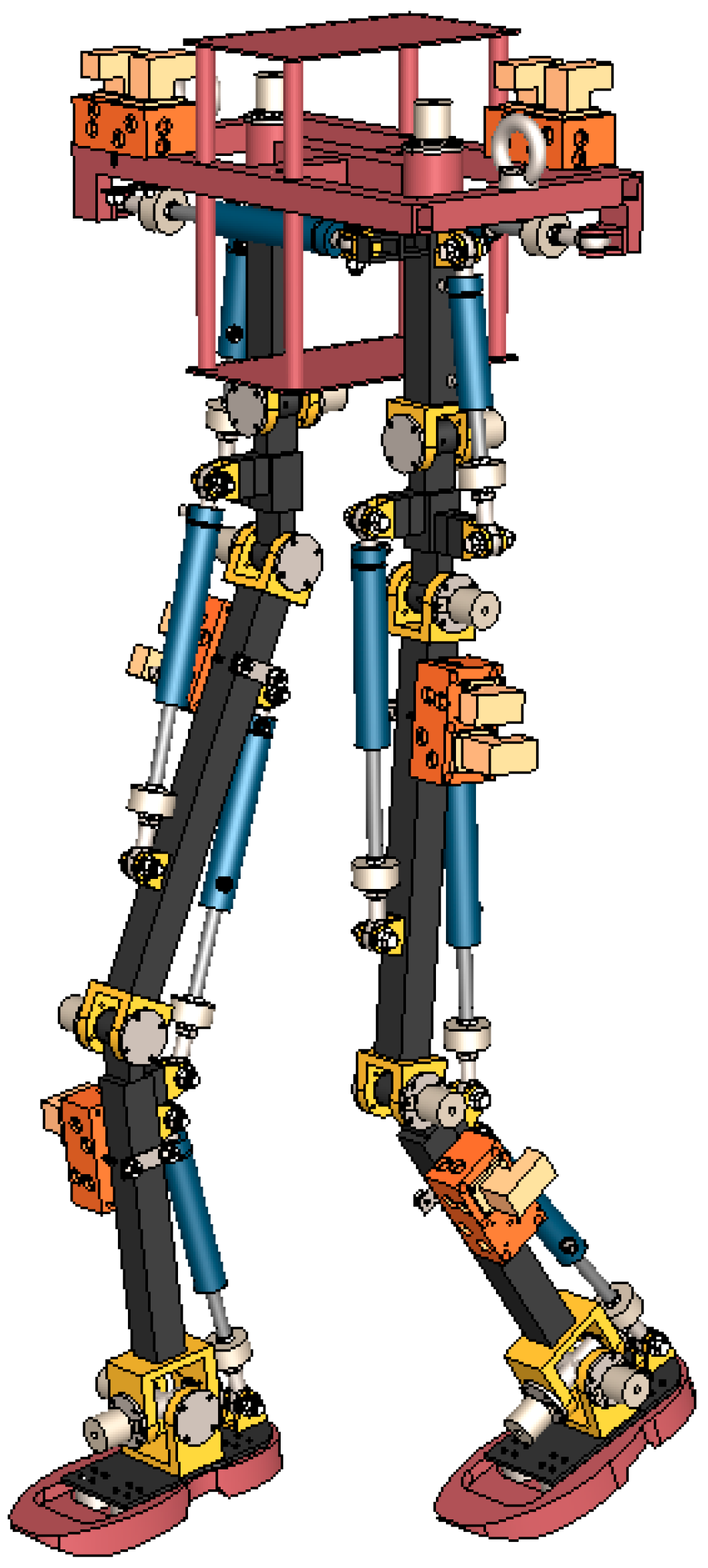
The hydraulically driven biped robot has 12 DOF, as shown in Figure 1, including 3DOF of hip joint, 1DOF of knee joint and 2DOF of ankle joint. To facilitate the calculation of the zero-moment point (ZMP), four miniature load cells (JHBM-M2 (300 kg)) are arranged on the sole. The baffle-force feedback electro-hydraulic flow control servo valve (FF102) is used as the three-position four-way reversing valve adopts, which is arranged in a distributed way to reduce the number of pipelines and the height of the robot’s center of gravity, thus effectively improving the robot’s walking stability.

2.1. Modular Joint Axis Design

The degree of freedom of the robot is determined by the number of joints. By adopting the modular structure of modular joint axis, it can reduce the cost of design and production, the modules are interchangeable, and the assembly is also quick and easy, which is beneficial to the maintenance and repair of the robot. Various joint shafts of the hydraulic biped robot adopt the same structure, as shown in Figure 2. Joint link 2 is connected to the articulated shaft with set screws, which can perform a relative rotational movement with Joint link 1. The magnitude of the rotational angular displacement is measured by an incremental hollow sleeve type encoder (EB38K). The encoders are installed on both ends of the joint axis.

2.2. Design of Drive/Test Parts

For the robot knee joint, the hydraulic cylinder is used as the driving device, as shown in Figure 3. To facilitate the measurement of the output force of the hydraulic cylinder, a bellows-type pull pressure sensor (JLBM-2 (1 T tension and compression)) is installed at the end of the piston rod. The two ends of the connecting rod are connected to the support lugs by joint bearings. Through the telescopic movement of the hydraulic cylinder, the joint link 1 and the joint link 2 can be rotated around the joint axis.

2.3. The Relationship between the Displacement of Hydraulic Cylinder and the Rotation Angle of Joint Axis

The drive input of the robot joint is the linear displacement of the hydraulic cylinder, and the position is detected by the rotation angle of the joint. In the robot controlling process, the relationship between the displacement of the hydraulic cylinder and the rotation angle of the joint axis needs to be calculated. The mechanism can be equivalent to a four-link mechanism, and taking the knee joint as an example, the mutual relationship is as shown in Figure 4. The relationship between the displacement of the hydraulic cylinder and the rotation angle of the joint axis is calculated as follows.

B is the knee joint, BC is the thigh, and BO is the calf, $\angle CBO=\theta , l_{AO}=65 \mathrm{mm}, l_{BO}=72 \mathrm{mm}, l_{BC}=385 \mathrm{mm}, l_{DC}=45 \mathrm{mm}$. According to the actual structural relationship, we can obtain: $\angle AOB=\angle BCD=90°$, and further obtain,

$$\begin{array}{c}{l}_{AB}=\sqrt{l_{AO}{}^2+l_{BO}{}^2}, l_{BD}=\sqrt{l_{BC}{}^2+l_{DC}{}^2}\end{array}$$

(1)

$$\begin{array}{c}\angle ABD+\angle ABO+\angle CBD=\theta , \theta \in \left[50°,180°\right]\end{array}$$

(2)

$$\begin{array}{c}\angle ABO=arc\tan \frac{l_{AO}}{l_{BO}}, \angle CBD=arc\tan \frac{l_{DC}}{l_{BC}}\end{array}$$

(3)

The length $l_{AD}$ of the joint link AD is determined by the expansion allowance of the hydraulic cylinder, and we can get,

$$\begin{array}{c}{l}_{AD}=\sqrt{l_{AB}{}^2+l_{BD}{}^2-2l_{AB}{l}_{BD}\cos \angle ABD}\end{array}$$

(4)

The relationship between the displacement of the hydraulic cylinder and the rotation angle of the joint axis is shown in Figure 5.

2.4. Finite Element Analysis of Critical Parts

When the robot is walking, deformation and fracture of the mechanism tend to occur at the weak link under the force of gravity and ground impact. The motion joint is the weakest link of the robot mechanism, so it is necessary to conduct a finite element analysis of the critical components in order to meet the application requirements. The material is 45# steel, the elastic modulus is 2.05 × 10¹¹ Pa, the Poisson’s ratio is 0.29, the shear modulus is 800 MPa, the mass density is 7.85 × 10³ kg/m³, and the yield strength is 530 MPa. The simulation module of SolidWorks software is used for finite element analysis, the solid mesh type is selected, and the element size is 4.7 mm.

The maximum ground impact force during human walking and running is about three times the weight of the human body, and there is sufficient safety margin. The loading force is 5 kN. The analysis results are listed in Figure 6. The finite element analysis results show that the maximum stress is smaller than the yield stress, and the strength of critical components meets the requirements.

3. Kinematics Analysis

The Denavit-Hartenberg (D-H) modeling method needs to establish a coordinate system for each joint, and each coordinate system has different posture. When the robot configuration changes, the model needs to be reestablished. Therefore, the D-H method involves a complicated process, low calculation efficiency, and unclear geometric meaning [25]. To a certain extent, it’s easier to use the screw theory to solve the kinematics of the humanoid robot is than to use the traditional D-H parameter method, because it does not need to establish one coordinate system for each link, and the entire system only has two coordinate systems (inertial coordinate system S and tool coordinate system T). Therefore, when analyzing complex spatial mechanisms, the screw theory can be employed to simplify and unify the description and solution of problems, which has more clear geometric meaning and higher numerical stability [26]. Based on the screw theory, the forward kinematics equation is obtained by using the product of exponential (POE) formula, and the velocity Jacobian matrix is derived.

3.1. Forward Kinematics

The coordinate system of the right leg is established in the form of the POE, as shown in Figure 7.

$\omega$ is the rotation axis of the rigid body, $r$ is any point on the axis, and Matrix $\left[V\right]$ is the twist produced by pure rotation, shown as:

$$\begin{array}{c}\left[V\right]=\left[\begin{array}{cc}\left[\omega \right]& v\\ 0& 0\end{array}\right]\end{array}$$

(5)

Here, the antisymmetric matrix $\left[\omega \right]\in so\left(3\right)$,$v=-\omega \times r$

The matrix index of the twist [V] is

$$\begin{array}{c}{\mathrm{e}}^{\left[V\right]\theta }=\left[\begin{array}{cc}R\left(\theta \right)& p\left(\theta \right)\\ 0& 1\end{array}\right]\end{array}$$

(6)

The rotation matrix is obtained by Rodrigues formula, namely

$$\begin{array}{c}R\left(\theta \right)={\mathrm{e}}^{\left[\omega \right]\theta }=I+\left[\omega \right]\sin \theta +{\left[\omega \right]}^2\left(1-cos\theta \right)\end{array}$$

(7)

The vector is calculated as follows:

$$\begin{array}{c}p\left(\theta \right)=\left(1-{\mathrm{e}}^{\left[\omega \right]\theta }\right)\left(\omega \times v\right)+\omega {\omega }^{T}v\theta \end{array}$$

(8)

The directions of the line vectors of various joint axes are:

$$\begin{array}{c}\begin{array}{c}{\omega }_1=\left[\begin{array}{c}0\\ 0\\ 1\end{array}\right],{\omega }_2={\omega }_6=\left[\begin{array}{c}1\\ 0\\ 0\end{array}\right],{\omega }_3={\omega }_4={\omega }_5=\left[\begin{array}{c}0\\ 1\\ 0\end{array}\right]\\ \left[{\omega }_1\right]=\left[\begin{array}{ccc}0& -1& 0\\ 1& 0& 0\\ 0& 0& 0\end{array}\right]\left[{\omega }_2\right]=\left[{\omega }_6\right]=\left[\begin{array}{ccc}0& 0& 0\\ 0& 0& -1\\ 0& 1& 0\end{array}\right]\\ \left[{\omega }_3\right]=\left[{\omega }_4\right]=\left[{\omega }_5\right]=\left[\begin{array}{ccc}0& 0& 1\\ 0& 0& 0\\ -1& 0& 0\end{array}\right]\end{array}\end{array}$$

(9)

Take one point on various joint axes as

$$\begin{array}{c}\begin{array}{c}{r}_1=\left[\begin{array}{c}0\\ -l_1\\ 0\end{array}\right],r_2=\left[\begin{array}{c}0\\ -l_1\\ -l_2\end{array}\right],r_3=\left[\begin{array}{c}0\\ -l_1\\ -l_2-l_3\end{array}\right]\\ r_4=\left[\begin{array}{c}0\\ -l_1\\ -l_2-l_3-l_4\end{array}\right],r_5=r_6=\left[\begin{array}{c}0\\ -l_1\\ -l_2-l_3-l_4-l_5\end{array}\right]\end{array}\end{array}$$

(10)

Under the shape and position when θ = 0, the transformation matrix of the tool coordinate system {T} relative to the basic coordinate system {S} is:

$$\begin{array}{c}{}_T{}^{S}T\left(0\right)=\left[\begin{array}{cccc}1& 0& 0& 0\\ 0& 1& 0& -l_1\\ 0& 0& 1& -l_2-l_3-l_4-l_5-l_6\\ 0& 0& 0& 1\end{array}\right]\end{array}$$

(11)

The twists of various joints are:

$$\begin{array}{c}{\mathrm{e}}^{\left[V_1\right]{\theta }_1}=\left[\begin{array}{cccc}cos{\theta }_1& -sin{\theta }_1& 0& -l_{1}sin{\theta }_1\\ sin{\theta }_1& cos{\theta }_1& 0& -l_1\left(1-cos{\theta }_1\right)\\ 0& 0& 1& 0\\ 0& 0& 0& 1\end{array}\right]\end{array}$$

(12)

$$\begin{array}{c}{\mathrm{e}}^{\left[V_2\right]{\theta }_2}=\left[\begin{array}{cccc}1& 0& 0& 0\\ 0& cos{\theta }_2& -sin{\theta }_2& -l_1\left(1-cos{\theta }_2\right)-l_{2}sin{\theta }_2\\ 0& sin{\theta }_2& cos{\theta }_2& l_{1}sin{\theta }_2-l_2\left(1-cos{\theta }_2\right)\\ 0& 0& 0& 1\end{array}\right]\end{array}$$

(13)

$$\begin{array}{c}{\mathrm{e}}^{\left[V_3\right]{\theta }_3}=\left[\begin{array}{cccc}cos{\theta }_3& 0& sin{\theta }_3& \left(l_2+l_3\right)sin{\theta }_3\\ 0& 1& 0& 0\\ -sin{\theta }_3& 0& cos{\theta }_3& -\left(l_2+l_3\right)\left(1-cos{\theta }_3\right)\\ 0& 0& 0& 1\end{array}\right]\end{array}$$

(14)

$$\begin{array}{c}{\mathrm{e}}^{\left[V_4\right]{\theta }_4}=\left[\begin{array}{cccc}cos{\theta }_4& 0& sin{\theta }_4& \left(l_2+l_3+l_4\right)sin{\theta }_4\\ 0& 1& 0& 0\\ -sin{\theta }_4& 0& cos{\theta }_4& -\left(l_2+l_3+l_4\right)\left(1-cos{\theta }_4\right)\\ 0& 0& 0& 1\end{array}\right]\end{array}$$

(15)

$$\begin{array}{c}{\mathrm{e}}^{\left[V_5\right]{\theta }_5}=\left[\begin{array}{cccc}cos{\theta }_5& 0& sin{\theta }_5& \left(l_2+l_3+l_4+l_5\right)sin{\theta }_5\\ 0& 1& 0& 0\\ -sin{\theta }_5& 0& cos{\theta }_5& -\left(l_2+l_3+l_4+l_5\right)\left(1-cos{\theta }_5\right)\\ 0& 0& 0& 1\end{array}\right]\end{array}$$

(16)

$$\begin{array}{c}{\mathrm{e}}^{\left[V_6\right]{\theta }_6}=\left[\begin{array}{cccc}1& 0& 0& 0\\ 0& cos{\theta }_6& -sin{\theta }_6& -l_1\left(1-cos{\theta }_6\right)-\left(l_2+l_3+l_4+l_5\right)sin{\theta }_6\\ 0& sin{\theta }_6& cos{\theta }_6& l_{1}sin{\theta }_6-\left(l_2+l_3+l_4+l_5\right)\left(1-cos{\theta }_6\right)\\ 0& 0& 0& 1\end{array}\right]\end{array}$$

(17)

It can be obtained from the POE formula that:

$$\begin{array}{c}{}_T{}^{S}T\left(\theta \right)={\mathrm{e}}^{\left[V_1\right]{\theta }_1}{\mathrm{e}}^{\left[V_2\right]{\theta }_2}\cdots {\mathrm{e}}^{\left[V_6\right]{\theta }_6}{}_T{}^{S}T\left(0\right)=\left[\begin{array}{cc}R\left(\theta \right)& p\left(\theta \right)\\ 0& 1\end{array}\right]\end{array}$$

(18)

In the above formula, the values are: l₁ = 125 mm, l₂ = 258.5 mm, l₃ = 164 mm, l₄ = 520 mm, l₅ = 422 mm, l₆ = 60 mm. The POE formula for the left leg can be established similarly as above.

3.2. Inverse Kinematics

For the kinematics model built based on the spin theory, its inverse solution is mainly solved based on the Paden-Kahan subproblem. However, the simple Paden-Kahan sub-problem can only be adopted to solve the inverse solution of humanoid robots with low degrees of freedom (no more than three degrees of freedom) [27]. In this paper, the method of analytical geometry is used to solve the inverse kinematics of the robot.

3.2.1. Sagittal Inverse Kinematics

In the sagittal plane, the knee joint angle of the right leg is θ4, and the position coordinates of the hip and ankle joints are known, as shown in Figure 8.

We get:

$$\begin{array}{c}cos\left({\theta }_4\right)=\frac{R^2-l_4^2-l_5^2}{2l_4{l}_5}\end{array}$$

(19)

From the inverse tangent function atan2, θ₄ can be obtained

$$\begin{array}{c}{\theta }_4=a\tan 2\left(\sqrt{1-{\left(\frac{R^2-l_4^2-l_5^2}{2l_4{l}_5}\right)}^2},\frac{R^2-l_4^2-l_5^2}{2l_4{l}_5}\right)\end{array}$$

(20)

where, $R^2={\left(x_3-x_5\right)}^2+{\left(z_3-z_5\right)}^2$.

The ankle angle θ₅ is composed of θ_a and θ_b, ${\theta }_a=a\tan 2\left(x_3-x_5,z_3-z_5\right)$, and ${\theta }_b=a\tan 2\left(l_4\sin {\theta }_4,l_5+l_4\cos {\theta }_4\right)$

$$\begin{array}{c}{\theta }_5={\theta }_a+{\theta }_b\end{array}$$

(21)

After calculating the knee joint angle θ₄ and the ankle joint angle θ₅, the next step is to calculate the hip joint angle θ₃. During the movement of the robot, the upper body needs to maintain a vertical posture all the time, so the sum of the ankle joint angle, knee joint angle, and hip joint angle is zero, and θ₃ can be calculated by

$$\begin{array}{c}{\theta }_3=-{\theta }_4-{\theta }_5\end{array}$$

(22)

The inverse kinematics of the left leg is obtained in a similar way as for the right leg, and we get:

$$\begin{array}{c}{\theta }_{l4}=a\tan 2\left(\sqrt{1-{\left(\frac{R_l^2-l_4^2-l_5^2}{2l_4{l}_5}\right)}^2},\frac{R_l^2-l_4^2-l_5^2}{2l_4{l}_5}\right)\end{array}$$

(23)

$$\begin{array}{c}{\theta }_{l5}=a\tan 2\left(x_{l3}-x_{l5},z_{l3}-z_{l5}\right)+a\tan 2\left(l_4\sin {\theta }_{l4},l_5+l_4\cos \theta l_4\right)\end{array}$$

(24)

$$\begin{array}{c}{\theta }_{l3}=-{\theta }_{l4}-{\theta }_{l5}\end{array}$$

(25)

where, θ_l4 is the knee joint angle of the left leg, θ_l5 is the ankle joint angle, and θ_l3 is the hip joint angle.

3.2.2. Coronary Inverse Kinematics

In the coronal plane, as shown in Figure 9, θ₆ is the ankle joint angle of the right leg, the height h of the hip joint relative to the ankle joint is known, and the distance between the two feet is l. We can get,

$$\begin{array}{c}{\theta }_6=a\tan 2\left(y_2-y_6,h\right)\end{array}$$

(26)

To ensure that the limb above the hip joint remains vertical, the angle of the knee joint in the coronal plane should not change, so the sum of the ankle joint angle and the hip joint angle is π/2. Therefore, the hip joint angle θ₂ can be calculated by the following equation,

$$\begin{array}{c}{\theta }_2=\frac{\pi }{2}-{\theta }_6\end{array}$$

(27)

Similarly, the joint angle θ_l2 and ankle joint angle θ_l6 of left leg can be calculated.

$$\begin{array}{c}{\theta }_{l6}=a\tan 2\left(y_{l2}-y_{l6},h\right)\end{array}$$

(28)

$$\begin{array}{c}{\theta }_{l2}=\frac{\pi }{2}-{\theta }_{l6}\end{array}$$

(29)

3.3. Speed Jacobian Matrix Based on POE Method

The speed Jacobian matrix (hereinafter referred to as Jacobian) refers to the mapping matrix from the speed of the driving joint to the speed of the end effector. As the core of the robot speed analysis, the establishment of the Jacobian matrix is the basis for kinematics analysis, acceleration analysis, accuracy analysis, static/dynamic analysis, and synthesis. The traditional way to describe a robot’s Jacobian matrix is to solve its forward kinematics using different equations, which involves a more complicated solving process and results in general. The screw theory can be employed to clearly describe the Jacobian matrix of the serial robot, which can highlight the geometric characteristics of the robot, and avoid the deficiencies of using local parameters in the differential method [28].

The screw theory and POE method can be used to easily solve the robot’s Jacobian matrix.

The POE formula of the robot kinematics equation is as follows:

$$\begin{array}{c}{}_T{}^{S}T\left(\theta \right)={\mathrm{e}}^{\left[V_1\right]{\theta }_1}{\mathrm{e}}^{\left[V_2\right]{\theta }_2}\cdots {\mathrm{e}}^{\left[V_6\right]{\theta }_6}{}_T{}^{S}T\left(0\right)=\left[\begin{array}{cc}R\left(\theta \right)& p\left(\theta \right)\\ 0& 1\end{array}\right]\end{array}$$

(30)

The instantaneous space velocity of the foot can be obtained.

$$\begin{array}{c}\left[{}_T{}^{S}V{}^s\right]={}_T{}^S\dot{T}\left(\theta \right){}_T{}^{S}T{}^{-1}\left(\theta \right)\end{array}$$

(31)

According to the characteristics of the POE formula of the kinematics equation, we get:

$$\begin{array}{c}\left[{}_T{}^{S}V{}^s\right]={\displaystyle {\displaystyle \sum }_{i=1}^n}\left(\frac{\partial \left({}_T{}^{S}T\right)}{\partial {\theta }_i}{\dot{\theta }}_i\right){}_T{}^{S}T{}^{-1}\left(\theta \right)={\displaystyle {\displaystyle \sum }_{i=1}^n}\left(\frac{\partial \left({}_T{}^{S}T\right)}{\partial {\theta }_i}{}_T{}^{S}T{}^{-1}\left(\theta \right)\right){\dot{\theta }}_i\left(i=1\cdots 6\right)\end{array}$$

(32)

The twist coordinate can be represented as:

$$\begin{array}{c}{}_T{}^{S}V{}^s={}_T{}^{S}J{}^s\left(\theta \right)\dot{\theta }\end{array}$$

(33)

where, the matrix ${}_T{}^{S}J{}^s\left(\theta \right)\in R^{6\times n}$ is the spatial Jacobian matrix of the foot.

$$\begin{array}{c}{}_T{}^{S}J{}^s\left(\theta \right)=\left[{\left(\frac{\partial \left({}_T{}^{S}T\right)}{\partial {\theta }_1}{}_T{}^{S}T{}^{-1}\left(\theta \right)\right)}^{\vee }{\left(\frac{\partial \left({}_T{}^{S}T\right)}{\partial {\theta }_2}{}_T{}^{S}T{}^{-1}\left(\theta \right)\right)}^{\vee }\cdots {\left(\frac{\partial \left({}_T{}^{S}T\right)}{\partial {\theta }_6}{}_T{}^{S}T{}^{-1}\left(\theta \right)\right)}^{\vee }\right]\end{array}$$

(34)

The operator $\left[ · \right]$ in square bracket indicates an antisymmetric matrix, and $\vee$ is its inverse operator.

It maps the joint velocity vector to the corresponding twist coordinate of the foot. Let $\left[V_i\right]\in se\left(3\right)$ be the unit twist, so any column of the spatial Jacobian matrix is as follows.

$$\begin{array}{ccc}\hfill \frac{\partial \left({}_T{}^{S}T\right)}{\partial {\theta }_i}{}_T{}^{S}T{}^{-1}\left(\theta \right)& =\hfill & {\mathrm{e}}^{\left[V_1\right]{\theta }_1}{\mathrm{e}}^{\left[V_2\right]{\theta }_2}\cdots {\mathrm{e}}^{\left[V_{i-1}\right]{\theta }_{i-1}}\frac{\partial }{\partial {\theta }_1}\left({\mathrm{e}}^{\left[V_i\right]{\theta }_i}\right){\mathrm{e}}^{\left[V_{i+1}\right]{\theta }_{i+1}}\cdots {\mathrm{e}}^{\left[V_6\right]{\theta }_6}{}_T{}^{S}T\left(0\right){}_T{}^{S}T{}^{-1}\left(\theta \right)\hfill \\ & =\hfill & {\mathrm{e}}^{\left[V_1\right]{\theta }_1}{\mathrm{e}}^{\left[V_2\right]{\theta }_2}\cdots {\mathrm{e}}^{\left[V_{i-1}\right]{\theta }_{i-1}}\left[V_i\right]\frac{\partial }{\partial {\theta }_1}\left({\mathrm{e}}^{\left[V_i\right]{\theta }_i}\right){\mathrm{e}}^{\left[V_{i+1}\right]{\theta }_{i+1}}\cdots {\mathrm{e}}^{\left[V_6\right]{\theta }_6}{}_T{}^{S}T\left(0\right){}_T{}^{S}T{}^{-1}\left(\theta \right)\hfill \\ & =\hfill & {\mathrm{e}}^{\left[V_1\right]{\theta }_1}{\mathrm{e}}^{\left[V_2\right]{\theta }_2}\cdots {\mathrm{e}}^{\left[V_{i-1}\right]{\theta }_{i-1}}\left[V_i\right]\frac{\partial }{\partial {\theta }_1}\left({\mathrm{e}}^{\left[V_i\right]{\theta }_i}\right){\mathrm{e}}^{-\left[V_{i-1}\right]{\theta }_{i-1}}\cdots {\mathrm{e}}^{-\left[V_1\right]{\theta }_1}\hfill \end{array}$$

(35)

Convert it to twist coordinates:

$$\begin{array}{c}{\left(\frac{\partial \left({}_T{}^{S}T\right)}{\partial {\theta }_i}{}_T{}^{S}T{}^{-1}\left(\theta \right)\right)}^{\vee }=A{d}_V\left({\mathrm{e}}^{\left[V_1\right]{\theta }_1}{\mathrm{e}}^{\left[V_2\right]{\theta }_2}\cdots {\mathrm{e}}^{\left[V_{i-1}\right]{\theta }_{i-1}}\right)V_i\end{array}$$

(36)

Then, the space Jacobian matrix of the robot can be obtained:

$$\begin{array}{c}{}_T{}^{S}J{}^s\left(\theta \right)=\left[\begin{array}{cccc}{V}_1{}^{\prime }& V_2{}^{\prime }& \cdots & V_6{}^{\prime }\end{array}\right]\end{array}$$

(37)

$$\begin{array}{c}{V}_i{}^{\prime }=A{d}_V\left({\mathrm{e}}^{\left[V_1\right]{\theta }_1}{\mathrm{e}}^{\left[V_2\right]{\theta }_2}\cdots {\mathrm{e}}^{\left[V_{i-1}\right]{\theta }_{i-1}}\right)V_i\left(i=1\cdots 6\right)\end{array}$$

(38)

By conducting adjoint transformation to the twist coordinate $V_i$ of the robot’s i-th joint, the i-th column $V_i{}^{\prime }$of the Jacobian matrix can be obtained.

$$\begin{array}{c}{V}_i{}^{\prime }=\left[\begin{array}{c}{r}_1{}^{\prime }\times {\omega }_1{}^{\prime }\\ {\omega }_1{}^{\prime }\end{array}\right]\end{array}$$

(39)

where, $r_i{}^{\prime }$ is the position vector of a point on the lower axis of current configuration, and ${\omega }_i{}^{\prime }$ is the unit vector of the joint axis direction of current configuration.

$$\begin{array}{c}{\omega }_i{}^{\prime }={\mathrm{e}}^{\left[{\omega }_1\right]{\theta }_1}{\mathrm{e}}^{\left[{\omega }_2\right]{\theta }_2}\cdots {\mathrm{e}}^{\left[{\omega }_{i-1}\right]{\theta }_{i-1}}{\omega }_i\left(i=1\cdots 6\right)\end{array}$$

(40)

$$\begin{array}{c}\left[\begin{array}{c}{r}_i{}^{\prime }\\ 1\end{array}\right]={\mathrm{e}}^{\left[V_1\right]{\theta }_1}{\mathrm{e}}^{\left[V_2\right]{\theta }_2}\cdots {\mathrm{e}}^{\left[V_{i-1}\right]{\theta }_{i-1}}\left[\begin{array}{c}{r}_i\left(0\right)\\ 1\end{array}\right]\left(i=1\cdots 6\right)\end{array}$$

(41)

Here, $r_i\left(0\right)$ is the position vector of a point on the lower axis of the initial configuration.

4. Gait Model

Humanoid robot systems are complex three-dimensional systems. To better understand their dynamic behavior, many simplified models have been proposed. The linear inverted pendulum (LIP) model proposed by S. Kajita [29] is often used to study gait. The model assumes that the vertical acceleration of the centroid is zero, thereby defining the analytical expression of the centroid and decoupling the sagittal and coronal equations.

In three-dimensional space, we approximately simplify the biped robot into a virtual three-dimensional linear inverted pendulum model (3D-LIPM), which is composed of the robot’s centroid m and the legs connected to the centroid whose mass is ignored, as shown in Figure 10. Assuming the inverted pendulum can rotate freely around the support point, the length of the leg can change according to the support force f.

4.1. Dynamic Modeling

The motion equation of the centroid is:

$$\begin{array}{c}\{\begin{array}{c}m\ddot{x}=\frac{x}{r}f=f_x\\ m\ddot{y}=\frac{y}{r}f=f_y\\ m\ddot{z}=\frac{z}{r}f-mg=f_z-mg\end{array}\end{array}$$

(42)

where, r is the distance from the centroid to the support point, and x, y, and z are the projection lengths of r in the three directions of the coordinate axis. When controlling the centroid of the robot, a constraint plane needs to be added. The equation is:

$$\begin{array}{c}z=k_{x}x+k_{y}y+z_c\end{array}$$

(43)

To make the centroid move along the plane, the acceleration of the centroid needs to be orthogonal to the normal vector of the constraint plane, so we get

$$\begin{array}{c}\left[\begin{array}{ccc}{f}_x& f_y& f_z-mg\end{array}\right]\left[\begin{array}{c}-k_x\\ -k_y\\ 1\end{array}\right]=0\end{array}$$

(44)

Solve the equation, substitute it into Equation (43), and we can get

$$\begin{array}{c}f=\frac{mgr}{z_c}\end{array}$$

(45)

By ensuring that the supporting force f is proportional to the leg length r, the centroid can move along the constraint plane, as shown in Figure 11.

According to Equations (42) and (43), the dynamic equation of the centroid at the horizontal plane can be obtained

$$\begin{array}{c}\{\begin{array}{c}\ddot{x}=\frac{g}{z_c}x\\ \ddot{y}=\frac{g}{z_c}y\end{array}\end{array}$$

(46)

This equation is a linear equation about z_c, and the intersection with the constraint plane is used as the only parameter. The slope parameter k_x, k_y of the constraint plane does not affect the plane motion of the centroid.

Solving the first formula of Equation (46), we can obtain:

$$\begin{array}{c}\{\begin{array}{c}x\left(t\right)=x\left(0\right)\cosh \left(\omega t\right)+\frac{1}{\omega }\dot{x\left(0\right)}\sinh \left(\omega t\right)\\ \dot{x\left(t\right)}=\omega x\left(0\right)\sinh \left(\omega t\right)+\dot{x\left(0\right)}\cosh \left(\omega t\right)\end{array}\end{array}$$

(47)

where, $\omega =\sqrt{\frac{g}{z_c}}$ is the reciprocal of the support time constant T of the gait cycle, which is related to the height of the centroid and the acceleration of gravity.

The displacement and velocity in the y-direction can be obtained using the same method.

4.2. Gait Support Time

In the walking process, the time required by the centroid from the moment when foot falls on the ground to the moment when foot leaves the ground needs to be found out. Assuming that the initial conditions ($x_0$, $\dot{x_0}$) and termination conditions ($x_1$, $\dot{x_1}$) are known, then we can get according to Equation (47):

$$\begin{array}{c}\begin{array}{c}{x}_1=x_0\cosh \left(\omega \tau \right)+\frac{1}{\omega }\dot{x_0}\sinh \left(\omega \tau \right)\\ \dot{x_1}=\omega x_0\sinh \left(\omega \tau \right)+\dot{x_0}\cosh \left(\omega \tau \right)\end{array}\end{array}$$

(48)

By utilizing the following hyperbolic function relation:

$$\begin{array}{c}\cosh \left(x\right)=\frac{e^x+e^{-x}}{2},\sinh \left(x\right)=\frac{e^x-e^{-x}}{2}\end{array}$$

(49)

Equation (48) can be written as follows

$$\begin{array}{c}\begin{array}{c}{x}_1=\frac{x_0+\frac{1}{\omega }\dot{x_0}}{2}{e}^{\omega \tau }+\frac{x_0-\frac{1}{\omega }\dot{x_0}}{2}{e}^{-\omega \tau }\\ \dot{x_1}=\frac{\omega x_0+\dot{x_0}}{2}{e}^{\omega \tau }-\frac{\omega x_0-\dot{x_0}}{2}{e}^{-\omega \tau }\end{array}\end{array}$$

(50)

From Equation (50), we get,

$$\begin{array}{c}{x}_1+\frac{1}{\omega }\dot{x_1}=\left(x_0+\frac{1}{\omega }\dot{x_0}\right)e^{\omega \tau }\end{array}$$

(51)

By solving the (51), we can get

$$\begin{array}{c}\tau =\frac{1}{\omega }\ln \frac{\omega x_1+\dot{x_1}}{\omega x_0+\dot{x_0}}\end{array}$$

(52)

4.3. Orbital Energy

If the initial speed is insufficient, the centroid of the inverted pendulum will return without reaching the position directly above the support point; if the initial speed is sufficient, the centroid of the inverted pendulum will continue to move forward after reaching the position directly above the support point. Therefore, the centroid reaches the support point at the minimum speed, that is, the robot centroid reaches directly above the ankle joint, and the relationship between the potential energy and the centroid motion can be calculated at this position.

Multiply both sides of the first formula of Equation (46) by $\dot{x}$, and obtain the following equations by integration:

$$\begin{array}{c}\dot{x}\left(\ddot{x}-\frac{g}{z_c}x\right)=0\end{array}$$

(53)

$$\begin{array}{c}{\displaystyle \int }\dot{x}\left(\ddot{x}-\frac{g}{z_c}x\right)dt=constant\end{array}$$

(54)

we can get

$$\begin{array}{c}\frac{1}{2}{\dot{x}}^2-\frac{g}{2z_c}{x}^2=constant=E\end{array}$$

(55)

where, E is the sum of kinetic energy and potential energy, which is called the orbital energy. The first term on the left is kinetic energy, and the second term is potential energy. In this calculation, it is assumed that unit mass has energy, so the mass of the centroid is ignored. When E ≤ 0, the centroid will return before reaching the support point. When E > 0, we can get the velocity of the centroid passing directly above the support point.

$$\begin{array}{c}\left|{\dot{x}}_{top}\right|=\sqrt{2E}\end{array}$$

(56)

4.4. Exchange of Support Legs

Although the motion of a linear inverted pendulum is determined only by its initial condition, we can still control its speed, because the initial condition can be modified by the ground-contact time. For walking with fixed step, the support exchange of quickened ground-contact will decelerate the walking speed, while the support exchange of a delayed ground-contact will accelerate the walking speed.

The relationship between the exchange of support legs and the movement of inverted pendulum can be calculated. As shown in Figure 11, the step size is s, the position of the centroid relative to the previous support point is x_f, and the speed of the centroid during the exchange is v_f. The support is exchanged instantly, so v_f is both the final speed of the previous support phase and the initial speed of the new support phase.

By defining the orbital energies before and after the exchange as E₁ and E₂ respectively, we can get:

$$\begin{array}{c}{E}_1=\frac{1}{2}{v}_f{}^2-\frac{g}{2z_c}{x}_f{}^2\end{array}$$

(57)

$$\begin{array}{c}{E}_2=\frac{1}{2}{v}_f{}^2-\frac{g}{2z_c}{\left(x_f-s\right)}^2\end{array}$$

(58)

when the orbital energies E₁ and E₂ were given, we can calculate the necessary exchange condition by eliminating v_f from Equations (57) and (58):

$$\begin{array}{c}{x}_f=\frac{z}{gs}\left(E_2-E_1\right)-\frac{s}{2}\end{array}$$

(59)

The speed at the exchange moment can be calculated by (57), and we get:

$$\begin{array}{c}{v}_f=\sqrt{2E_1+\frac{g}{z_c}{x}_f{}^2}\end{array}$$

(60)

4.5. Generation of 3D Gait Model

Assuming that the robot walks at a constant support exchange speed, T_sup represents the support period of each step. A trajectory of the centroid during the support period is shown in Figure 12, which is symmetric around the y-axis, and the support time is [0 T_sup]. The end position is ($\overline{x},\overline{y}$), the end speed is (${\overline{v}}_x,{\overline{v}}_y$), according to the characteristics of symmetry, the initial condition along the x-axis is $\left(-\overline{x},{\overline{v}}_x\right)$, and the end position is $\overline{x}$. According to the analytical solution of the linear inverted pendulum, we can get:

$$\begin{array}{c}\overline{x}=-\overline{x}\cosh \left(\omega t\right)+\frac{1}{\omega }{\overline{v}}_x\sinh \left(\omega t\right)\end{array}$$

(61)

Solve the above equation to obtain the end velocity ${\overline{v}}_x$:

$$\begin{array}{c}{\overline{v}}_x=\frac{\omega \overline{x}\left(1+\cosh \left(\omega t\right)\right)}{\sinh \left(\omega t\right)}\end{array}$$

(62)

Similarly, the initial condition along the y-axis is $\left(\overline{y},-{\overline{v}}_y\right)$, and the end position is $\overline{y}$. We can get the end velocity:

$$\begin{array}{c}\begin{array}{c}\overline{y}=\overline{y}\cosh \left(\omega t\right)+\frac{1}{\omega }\left(-{\overline{v}}_y\right)\sinh \left(\omega t\right)\\ {\overline{v}}_y=\frac{\omega \overline{y}\left(\cosh \left(\omega t\right)-1\right)}{\sinh \left(\omega t\right)}\end{array}\end{array}$$

(63)

4.6. Walking Parameters

In real situations, such as climbing stairs or avoiding obstacles, it is often necessary to directly specify the position of the feet.

As shown in Figure 13, the position of a simple walking foot is represented by length and width of the step. For a normal person, the step length is generally within the range 500~800 mm, and the step width is within 80 ± 35 mm. The used data are listed in

Table 1. Foot position data.

n	0	1	2	3	4	5
$s_x^{\left(n\right)}$	0	0	500	500	500	0
$s_y^{\left(n\right)}$	0	100	100	100	100	100

.

In Table 1, s_x represents the step length in the walking direction, s_y represents the step width in the lateral direction, superscript (n) represents the n-th step, and the position of foot at the n-th step can be expressed as $(p_x^{\left(n\right)},p_y^{\left(n\right)})$:

$$\begin{array}{c}\left[\begin{array}{c}{p}_x^{\left(n\right)}\\ p_y^{\left(n\right)}\end{array}\right]=\left[\begin{array}{c}{p}_x^{\left(n-1\right)}+s_x^{\left(n\right)}\\ p_y^{\left(n-1\right)}-{\left(-1\right)}^n{s}_y^{\left(n\right)}\end{array}\right]\end{array}$$

(64)

where, $\left(p_x^{\left(0\right)},p_y^{\left(0\right)}\right)$ is the position of the first supporting foot, and Figure 13 shows the right foot. If the first supporting foot is the left foot, then −(−1)ⁿ needs to be replaced with +(−1)ⁿ in the formula.

The foot position at n-th step is:

$$\begin{array}{c}\left[\begin{array}{c}{\overline{x}}^{\left(n\right)}\\ {\overline{y}}^{\left(n\right)}\end{array}\right]=\left[\begin{array}{c}\frac{s_x^{\left(n+1\right)}}{2}\\ \frac{{\left(-1\right)}^n{s}_y^{\left(n+1\right)}}{2}\end{array}\right]\end{array}$$

(65)

It is worth noting that the foot position at the n-th step is determined by the step length and step width of the (n + 1)-th step, which is necessary for proper adjustment of the foot position and walking movement. The velocity formula at the end point is:

$$\begin{array}{c}\left[\begin{array}{c}{\overline{v}}_x^{\left(n\right)}\\ {\overline{v}}_y^{\left(n\right)}\end{array}\right]=\left[\begin{array}{c}\frac{\omega \left(1+\cosh \left(\omega t\right)\right)}{\sinh \left(\omega t\right)}{\overline{x}}^{\left(n\right)}\\ \frac{\omega \left(\cosh \left(\omega t\right)-1\right)}{\sinh \left(\omega t\right)}{\overline{y}}^{\left(n\right)}\end{array}\right]\end{array}$$

(66)

4.7. Modification of Foot Placements

For a robot walking with a fixed gait cycle, its speed can be controlled by adjusting the foot placements. Define the adjusted foot drop position as P_x, which is also the zero-torque point (ZMP) in the x-direction, and the centroid position is x_c, as shown in Figure 14.

From Equation (42), the dynamic equation along the x-direction is

$$\begin{array}{c}{\ddot{x}}_c=\frac{g}{z_c}\left(x_c-p_x\right)\end{array}$$

(67)

Its analytical solution is,

$$\begin{array}{c}\{\begin{array}{c}{x}_c\left(t\right)=(x_i^{\left(n\right)}-p_x)\cosh \left(\omega t\right)+\frac{1}{\omega }{\dot{x}}_i^{\left(n\right)}\sinh \left(\omega t\right)+p_x\\ {\dot{x}}_c\left(t\right)=\omega ({\dot{x}}_i^{\left(n\right)}-p_x)\sinh \left(\omega t\right)+{\dot{x}}_i^{\left(n\right)}\cosh \left(\omega t\right)\end{array}\end{array}$$

(68)

Equation (68) is written in the form of a state equation, and the relationship between the position $p_x$ and the end state of the n-th step can be obtained

$$\begin{array}{c}\left[\begin{array}{c}{x}_f^{\left(n\right)}\\ {\dot{x}}_f^{\left(n\right)}\end{array}\right]=\left[\begin{array}{cc}\cosh \left(\omega t\right)& \frac{1}{\omega }\sinh \left(\omega t\right)\\ \omega \sinh \left(\omega t\right)& \cosh \left(\omega t\right)\end{array}\right]\left[\begin{array}{c}{x}_i^{\left(n\right)}\\ {\dot{x}}_i^{\left(n\right)}\end{array}\right]+\left[\begin{array}{c}1-\cosh \left(\omega t\right)\\ -\omega \sinh \left(\omega t\right)\end{array}\right]p_x\end{array}$$

(69)

Here, $\omega =\sqrt{\frac{g}{z_c}}$ is the reciprocal of the support time constant T of the gait cycle. $x_i^{\left(n\right)}$ and ${\dot{x}}_i^{\left(n\right)}$ are the initial position and velocity of the n-th step, which are called the initial conditions.

As the target state, it can be represented by the end state in the ground coordinate system.

$$\begin{array}{c}\left[\begin{array}{c}{x}^d\\ {\dot{x}}^d\end{array}\right]=\left[\begin{array}{c}{p}_x^{\left(n\right)}+{\overline{x}}^{\left(n\right)}\\ {\overline{v}}_x^{\left(n\right)}\end{array}\right]\end{array}$$

(70)

The calculated final position of the foot is close to the target position, and the evaluation function defined below is adopted,

$$\begin{array}{c}N=a{(x^d-x_f^{\left(n\right)})}^2+b{({\dot{x}}^d-{\dot{x}}_f^{\left(n\right)})}^2\end{array}$$

(71)

where, a and b are positive. By substituting (69) into the evaluation function, let $\partial N/\partial p_x=0$, and we can get the position of the foot when N is minimum.

$$\begin{array}{c}{p}_x=-\frac{a\left(C-1\right)}{a{\left(C-1\right)}^2+b{\omega }^2{\mathrm{S}}^2}\left(x^d-x_i^{\left(n\right)}\mathrm{C}-\frac{1}{\omega }{\dot{x}}_i^{\left(n\right)}\mathrm{S}\right)-\\ \frac{b\omega S}{a{\left(\mathrm{C}-1\right)}^2+b{\omega }^2{\mathrm{S}}^2}\left({\dot{x}}^d-\omega x_i^{\left(n\right)}\mathrm{S}-{\dot{x}}_i^{\left(n\right)}\mathrm{C}\right)\end{array}$$

(72)

where, it is assumed that $\mathrm{C}=\cosh \left(\omega t\right)$,$\mathrm{and} \mathrm{S}=\sinh \left(\omega t\right)$.

The method of walking pattern generation can be organized as an algorithm shown as follows.

Step 1.

Set support period T_sup and walk parameters s_x, s_y. Set initial position $\left(x,y\right)$of CoM and initial foot placement $\left(p_x,p_y\right)=(p_x^{\left(0\right)},p_y^{\left(0\right)})$.

Step 2.

T = 0, n = 0.

Step 3.

Integrate the linear inverted pendulum Equation (67) (and the equation for the y-axis) from T to T + T_sup.

Step 4.

T = T + T_sup, n = n + 1.

Step 5.

Calculate the position $(p_x^{\left(n\right)},p_y^{\left(n\right)})$ for next foot using (64).

Step 6.

Set the ideal position parameter (${\overline{x}}^{\left(n\right)},{\overline{y}}^{\left(n\right)})$ for next step using (65) and (66).

Step 7.

Calculate the target state $(x^d,{\dot{x}}^d)$ using (70), and calculate the target state $(y^d,{\dot{y}}^d)$ using corresponding equation.

Step 8.

Calculate the modified foot position $\left(p_x,p_y\right)$ by (72) (as well as y component).

Step 9.

Go to Step 3.

5. Simulation Analysis

Based on the above model and algorithm analysis, simulation was conducted in the MATLAB software through programming. The simulated virtual environment is flat ground without any barrier, and the simplified model has the weight of 27.13 kg, the height of 1.42 m and the centroid height of 0.76 m. In the simulation, the following parameters are set: the step size is 0.5 m, the stride width is 0.25 m, the foot swing height is 0.05 m, the static friction coefficient between foot bottom and ground is 1, and the dynamic friction coefficient is 0.8. The generated centroid and the feet trajectory are shown in Figure 15. During the walking process, the angle changes of various joints are presented in Figure 16. Through simulation, it was found that the biped robot can walk steadily, as shown in Figure 17, which verifies the correctness of kinematics and 3D-LIPM and has laid the foundation for further analysis of stability.

6. Discussion

The hydraulic biped robot with innovative design has the characteristics of simple structure, fast motion speed and strong load capacity. The configuration of distributed hydraulic valve and valve block has effectively reduced the height of centroid and improved the walk stability of biped robot, and the position or force feedback of robot can be realized using this configuration. The shortage is that the overall weight of robot is higher. Restricted by the structural size, the motion range of mechanical joints has not completely reached the motion range of human joins at present.

For the forward kinematics solution of robot, if the D-H method is used to establish the coordinate system, it involves a complicated process, low efficiency, and no universality. Therefore, we employ the product of exponentials (PoE) method based on the screw theory to build the forward kinematics model of robot, which is easy to understand with clear geometric significance. When solving the inverse kinematics of robot, in order to prevent excessive dependency on the Paden-Kahan sub-problem, the analytical geometry method is adopted when the motion trail of hip joint and ankle joint is known, which can easily obtain the inverse kinematics solution. This method has provided a reference for the forward kinematics and inverse kinematics solutions of similar biped robots, which has great universality.

For the gait analysis of humanoid robot, the 3D-LIPM with broad application is used, and the ZMP theory is combined for gait planning. This method has simplified the model to a certain extent. Through simulation, the problems in the mathematical model and 3D model can be found in a timely manner, so that corresponding modification and improvement can be made. In order to demonstrate the simulation program in a physical model, and the model also needs to be further optimized. In addition, falling-prevention measures should also be taken to prevent damaging the robot.

7. Conclusions and Future Works

7.1. Conclusions

We propose a new hydraulic-driven biped robot, and because it involves too many components, we only conduct finite element analysis of the critical components at modular joints under bigger force and with relatively weaker structure. The loading force is the maximum impact on the robot during walking, and certain safety factors are kept. According to the analysis results, the maximum stress on critical components is lower than their allowable stress, which satisfies the strength condition.

The forward kinematics and Jacobian matrix formulas are inferred based on the screw theory. The analytical geometry method is adopted to easily obtain the inverse kinematics solution, which has provided the mathematical basis for gait planning and simulation. This method can also be used in biped robot models with similar structures.

A three-dimensional linear inverted pendulum model (3D-LIPM) is built for gait planning in the 3D space. Based on the MATLAB software platform, programming and simulation are adopted to verify the accuracy of kinematics and 3D-LIPM. The simulation results show that this biped robot can walk steadily on flat ground, which has not only laid down the basis for further verification in a physical model, but also provided basic data to conduct gait training of biped robot based on deep reinforcement learning theory in the future.

7.2. Future Works

7.2.1. Design of Mechanical Structure

The varus and valgus motions of ankle joint is underactuated, and in order to improve the controllability of mechanism, we will consider adding this actuation device in the next step. The angle sensor of modular joint is external, although it can satisfy the measurement requirement, it affects the appearance of structure, and the sensor might also be damaged if the robot falls, so we consider designing a built-in sensor in the next step.

7.2.2. Gait Model

The gait model was only simulated on flat ground, and further gait planning should also be conducted on slope, turning, stairs and uneven ground to improve the theoretical model. The 3D-LIPM model will be used for simulation in complicated environment, the stability research will be conducted, and the external environment for biped robot will be simulated in a more realistic way.

7.2.3. Simulation Model

The simulation model is a simplified version of a real robot, the hydraulic cylinder-driven part and the specific internal structure of joint are left out, and factors such as joint friction and joint space are not considered either. These factors will be included in subsequent simulations to more realistically simulate the actual state of biped robot.

7.2.4. Experimental Verification

Based on improvement of mechanical structure and optimization of gait mode, the control program will be generated for verification in physical model, so that the shortages of the theoretical model and physical model during the walking process can be found, the theoretical model and mechanical structure can be further optimized, and the biped robot can have better robustness.

8. Patents

Lower limb mechanism of a position and force controlled hydraulic biped robot, ZL201922274258.1.