Mini Wind Harvester and a Low Power Three-Phase AC/DC Converter to Power IoT Devices: Analysis, Simulation, Test and Design

 ,
,
Abstract
:1. Introduction
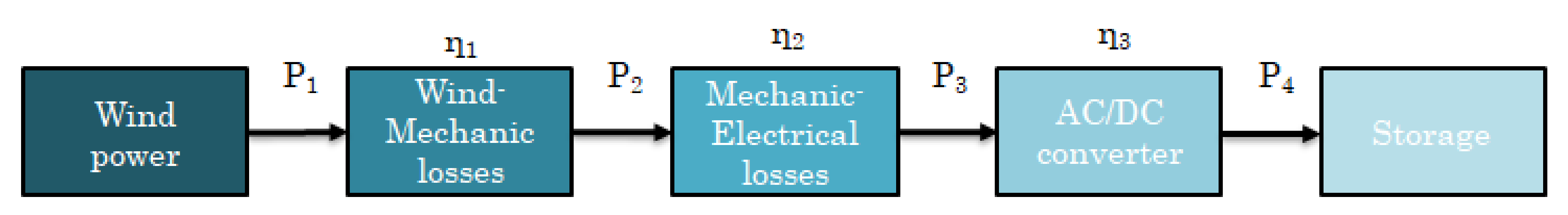
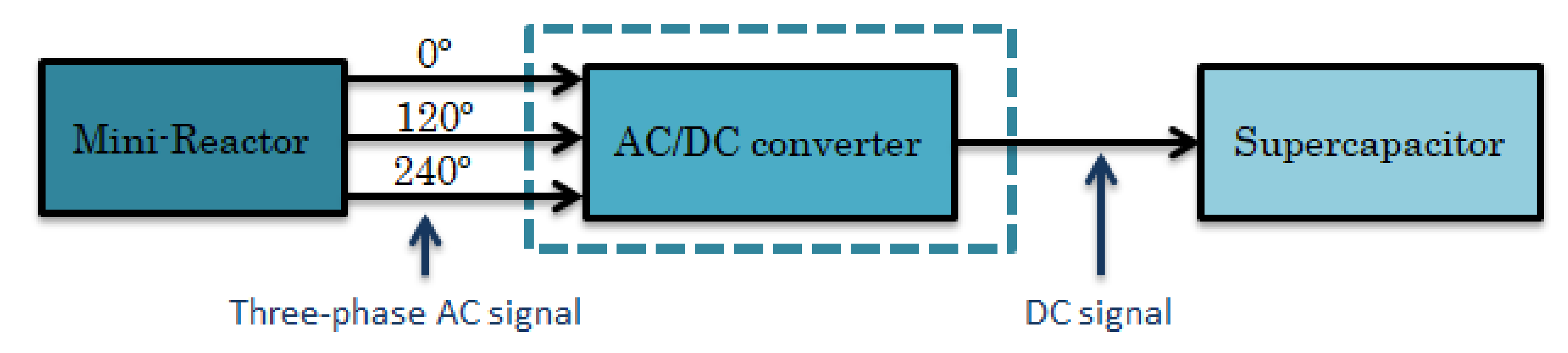
2. Harvesting System
3. Mini Wind Harvester Electro-Mechanical Three-Phase Model, Simulation, and Comparison with Test Results
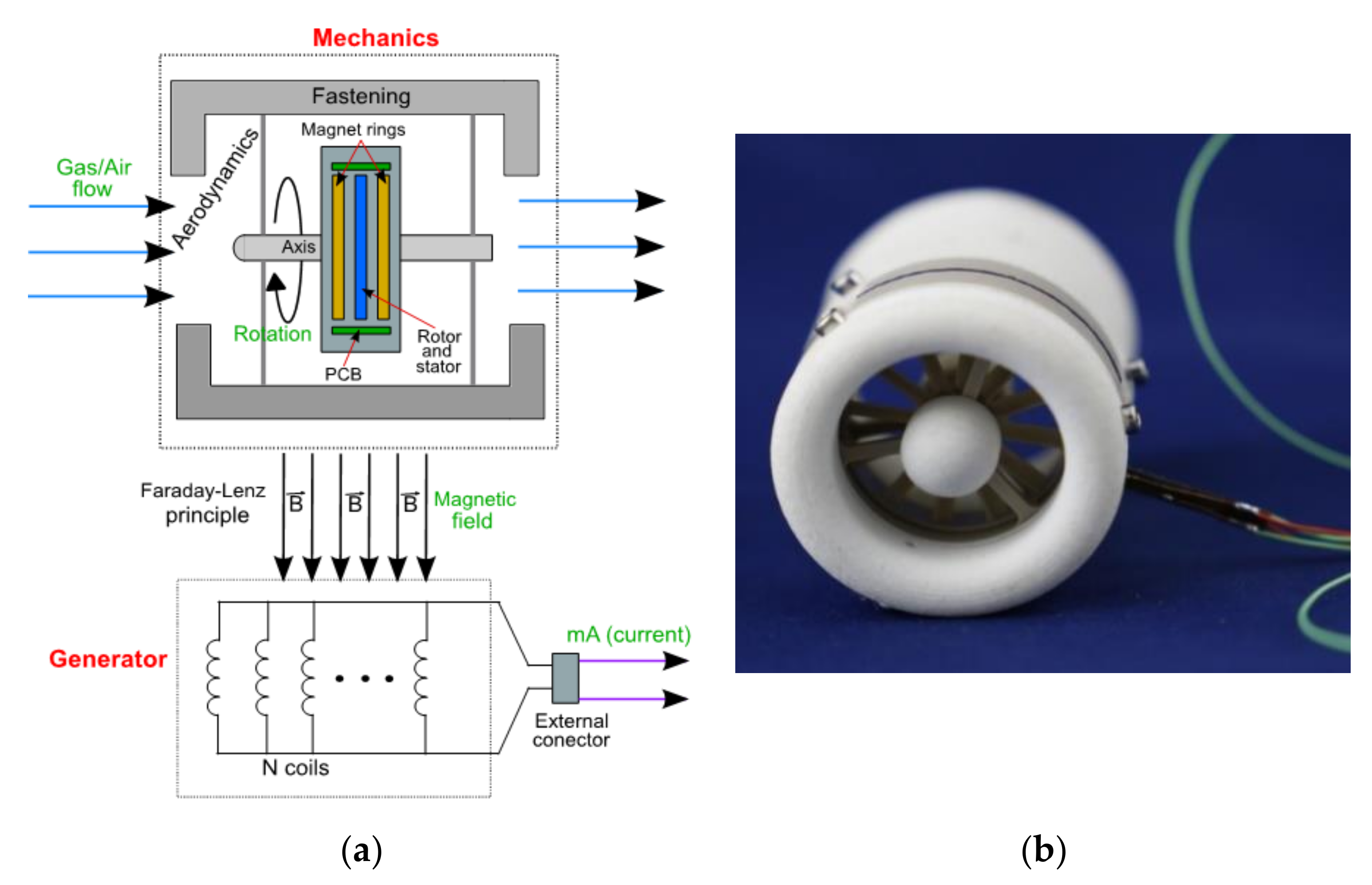
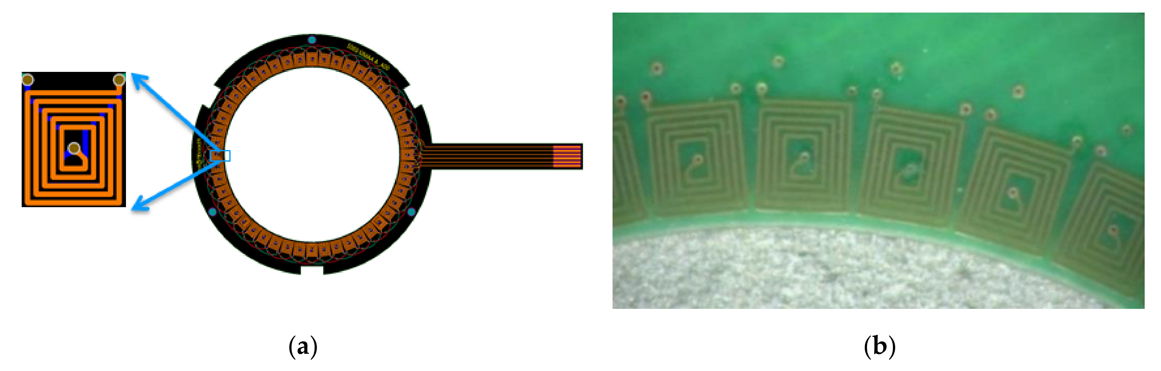
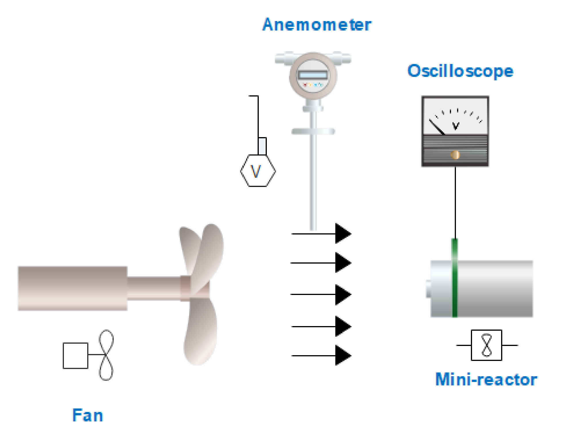
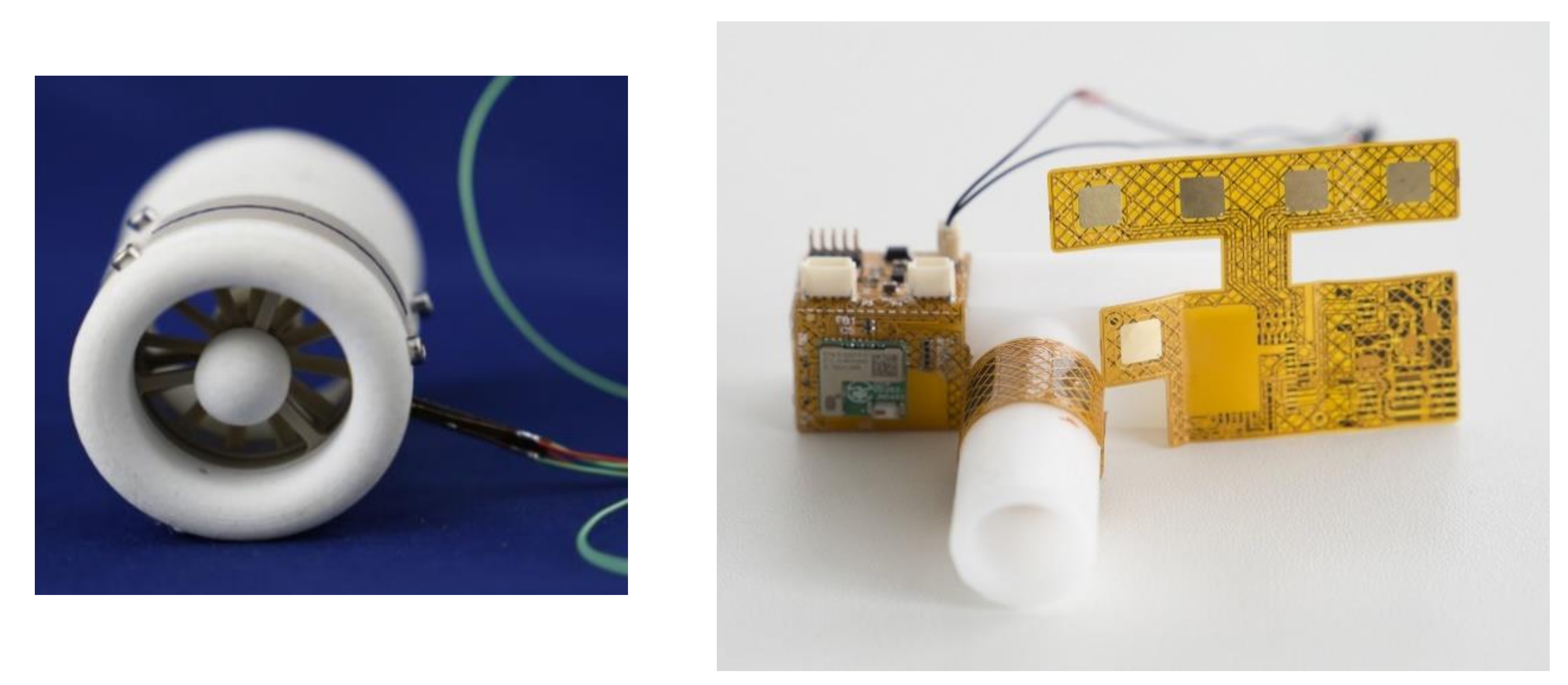
3.1. Mini Wind Harvester Description
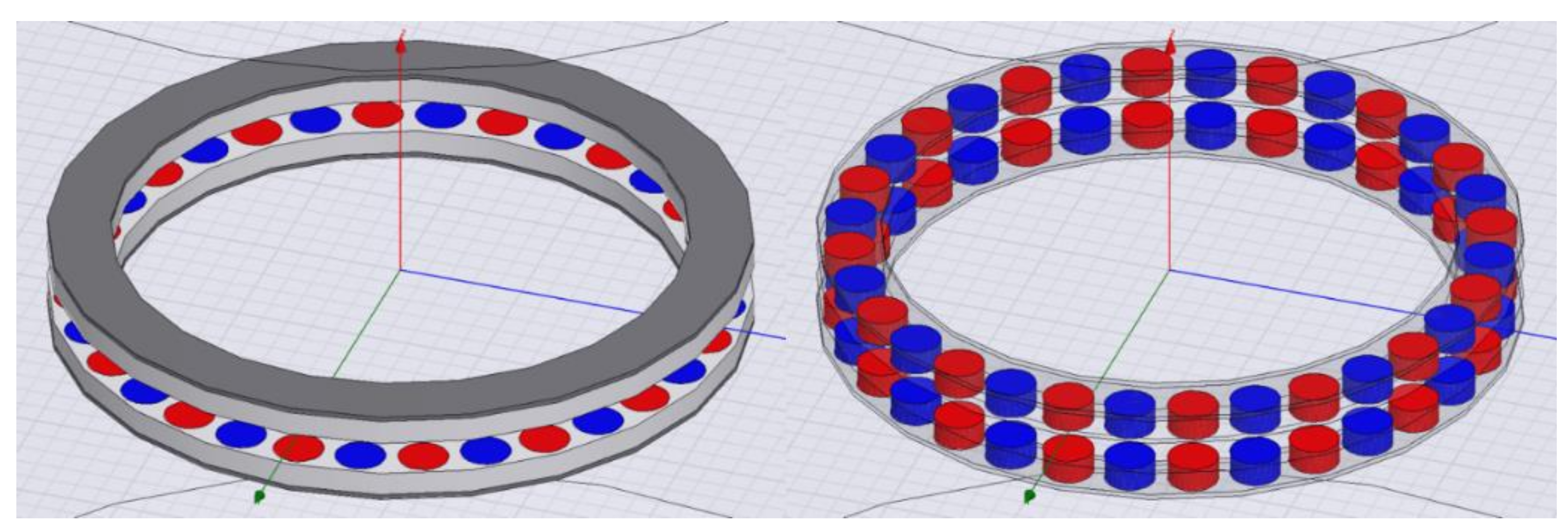
- The red and blue magnets have opposite polarity to generate an alternating magnetic flux when a continuous rotational movement is produced.
- The opposite magnets in two rings have the same polarity in order to not override the magnetic field in the center.
3.2. Theoretical Principles of Mini Wind Harvester Operation
3.2.1. Work Operation at Open Space Environment
- Wind velocity → 3 m/s and 4 m/s
- Resistive load → 36 Ω and 1e6 Ω (1 × 10⁶ Ω)
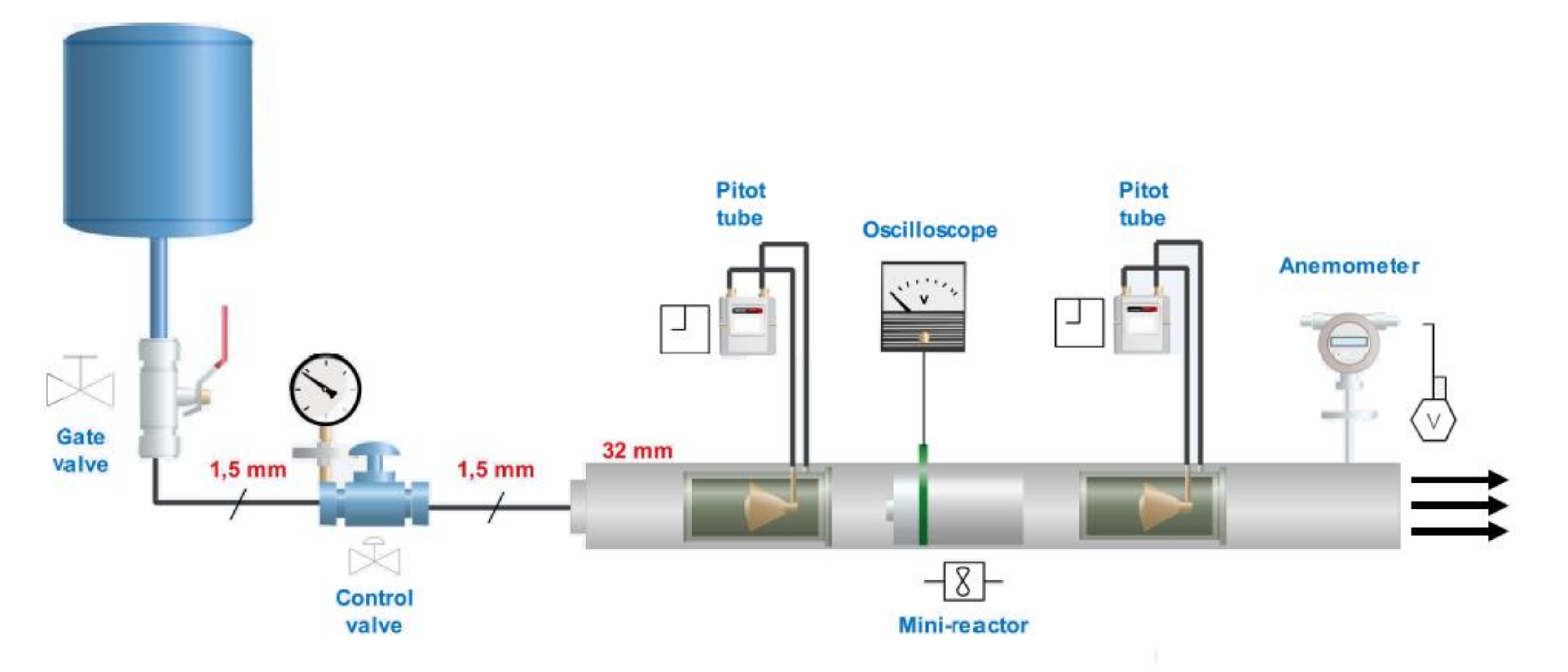
3.2.2. Work Operation inside a Closed Environment
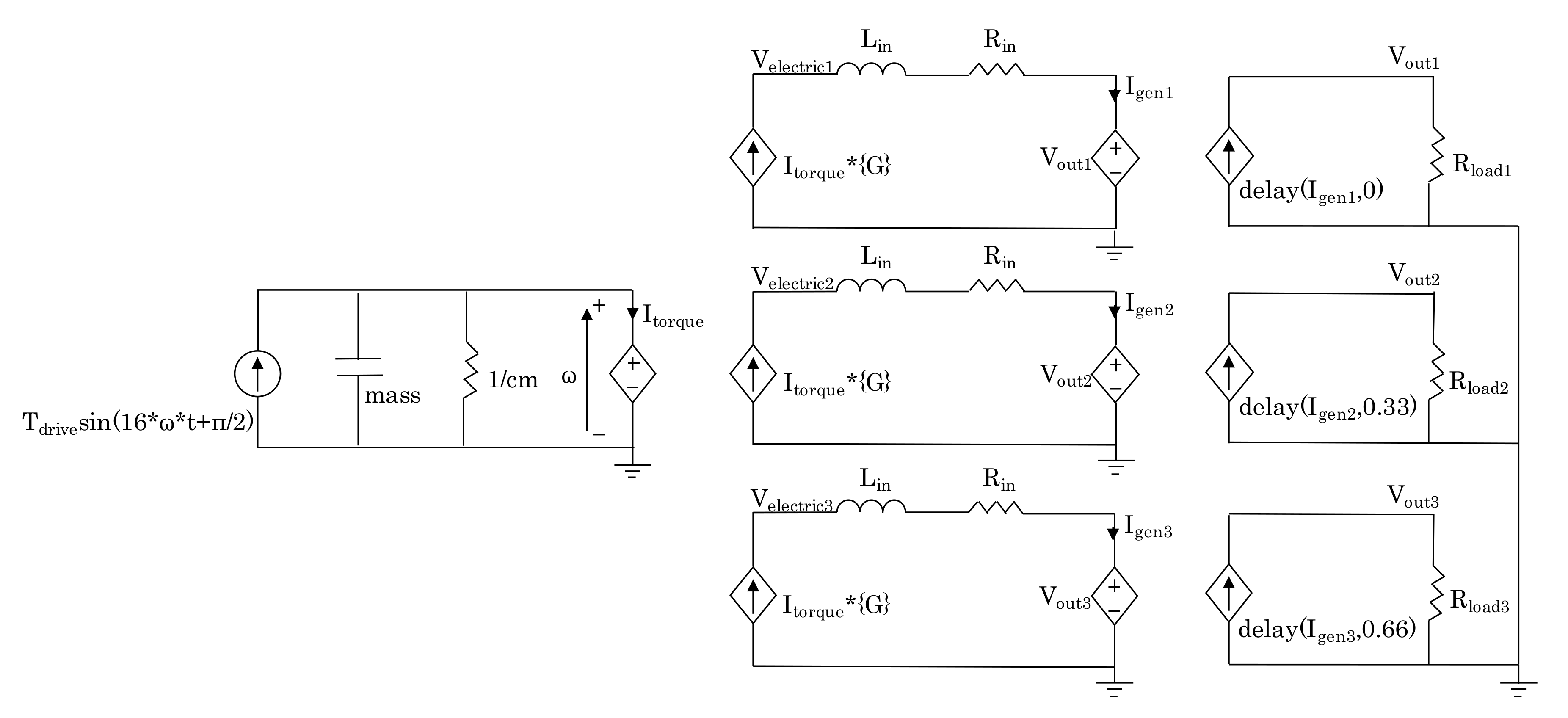
3.3. Electro-Mechanical Equivalent Model of the Mini Wind Harvester or Reactor
3.3.1. Equivalent Model Description
3.3.2. Parameters Measurement and Obtainment
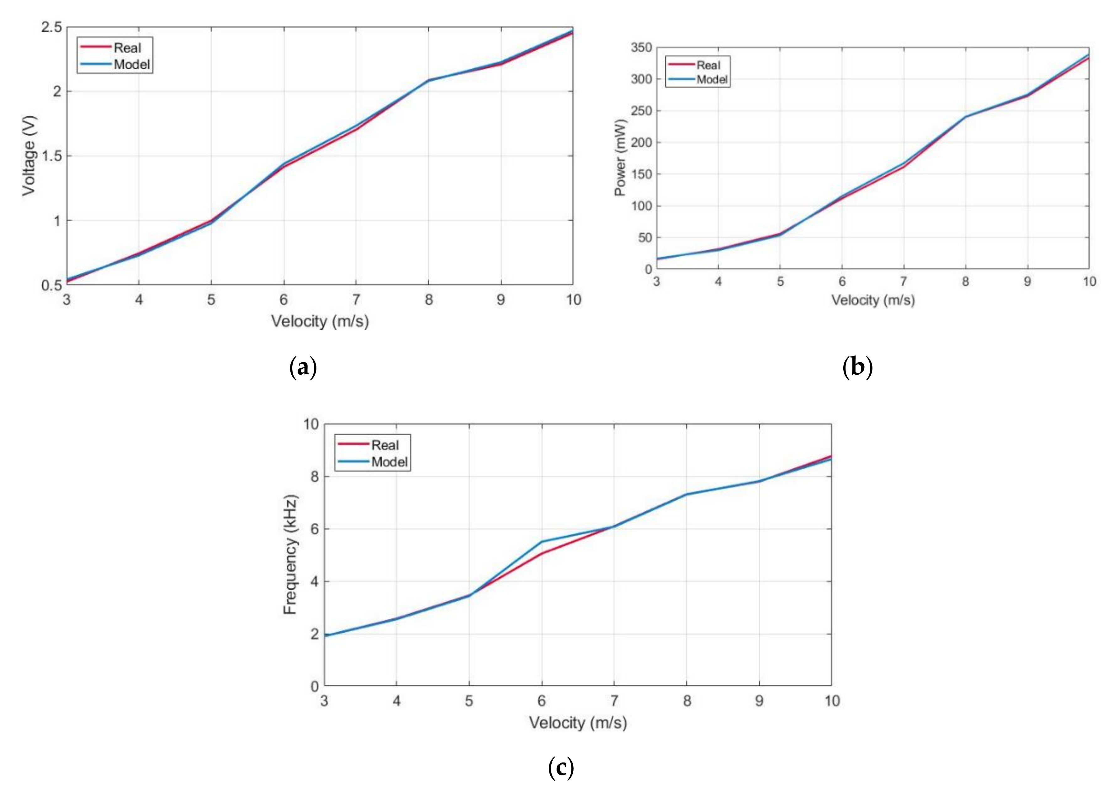
3.4. Model and Test Results Comparison and Proposed System Verification
4. AC/DC Converter
- A low-value coil: only 2 µH. The harvester’s own coil is used in order to avoid the losses of including another one.
- A low input AC voltage for energy harvesting the usual converters (voltage levels are between 0.3 V and 1.5 V, commercial diodes do not work properly in the rectification step with such low voltage levels due to the internal losses or the forward voltage, VF).
- An 8 kHz range frequency input: switching frequency changing.
- The influence of the reactive power of the generator must be considered.
- A minimum wind velocity condition of 3 m/s, i.e., when available input power is the minimum possible, because at lower wind velocity the generator rotatory movement does not generate enough power to start working the electronic system.
- A maximum wind velocity condition of 10 m/s, i.e., when available input power is the maximum possible, basically to ensure the mechanical integrity of the bearings. At this wind velocity the achieved angular velocity is 32.87 krpm and the harvester bearing is ensured until 35 krpm of angular velocity.
4.1. Operation Principles of AC/DC Converters Architectures
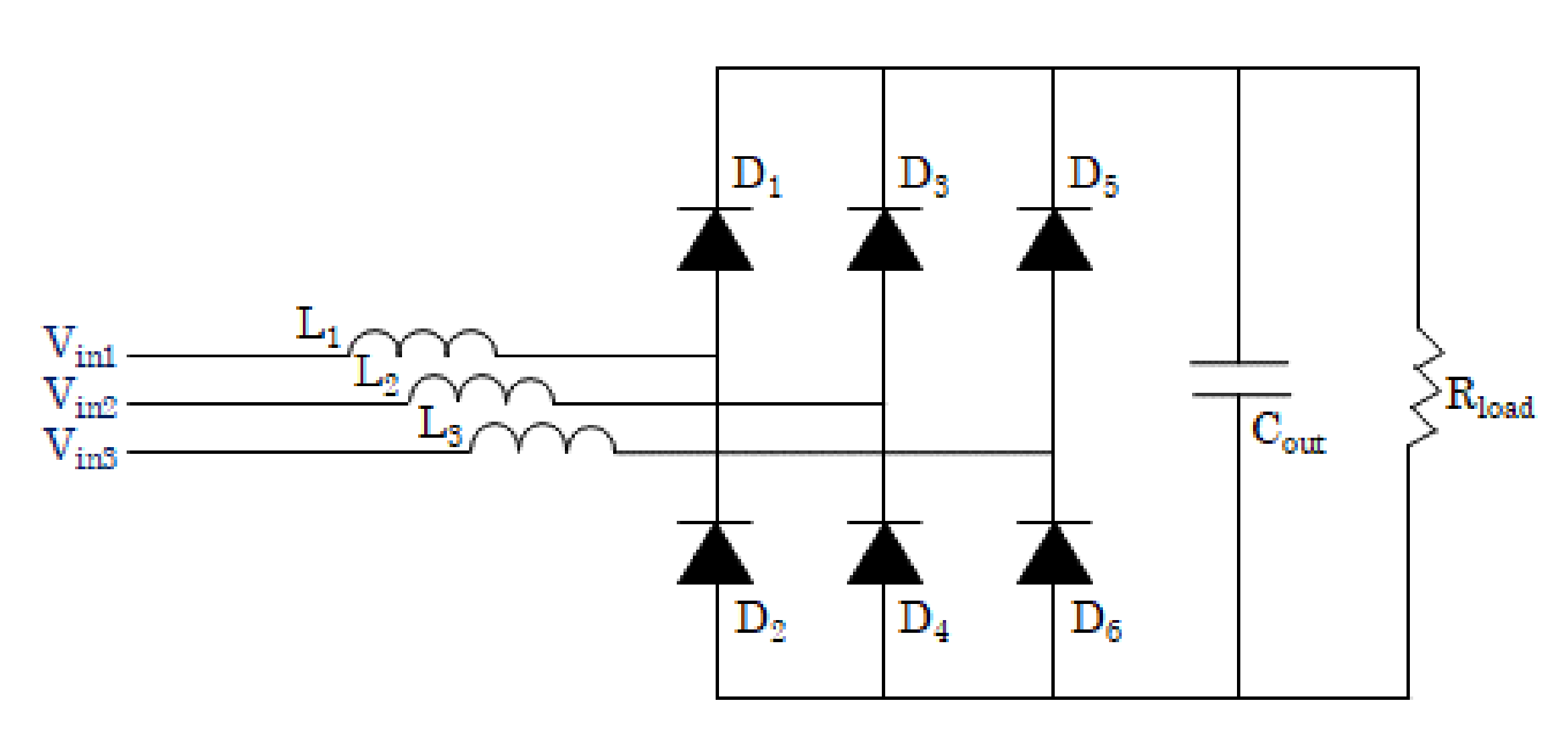
4.1.1. Three Phase Diode Bridge
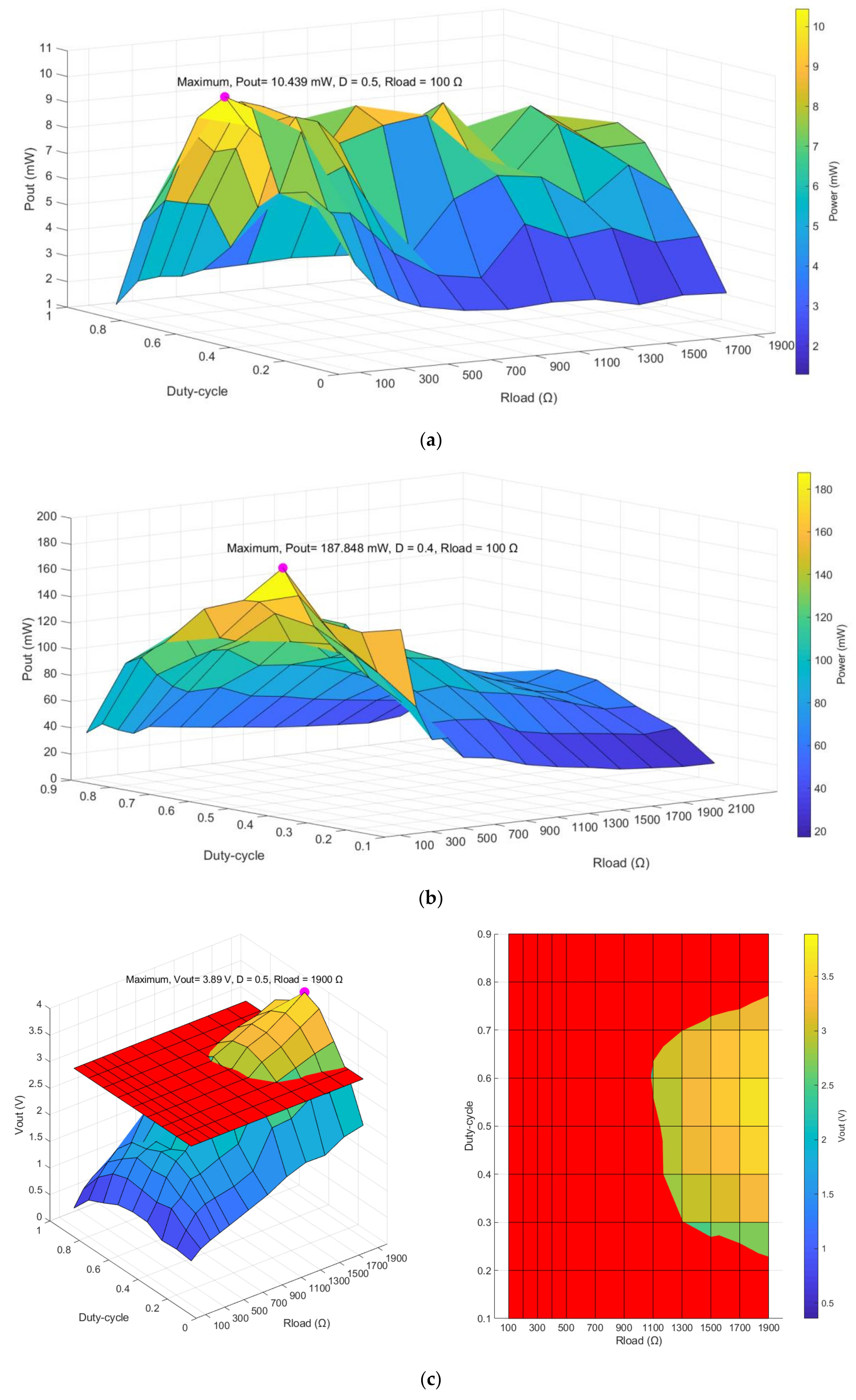
4.1.2. Secondary Side Diode-Based Topology
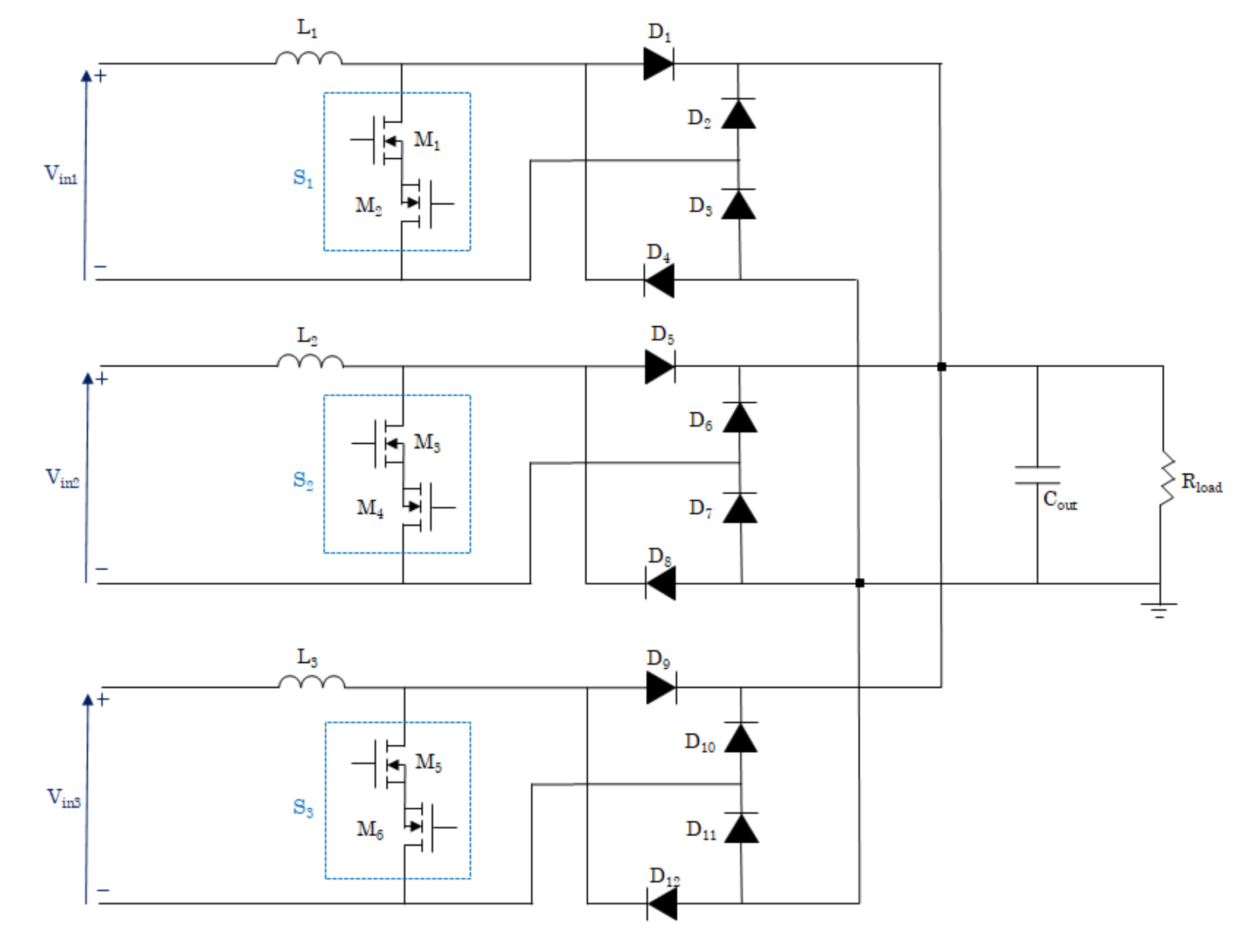
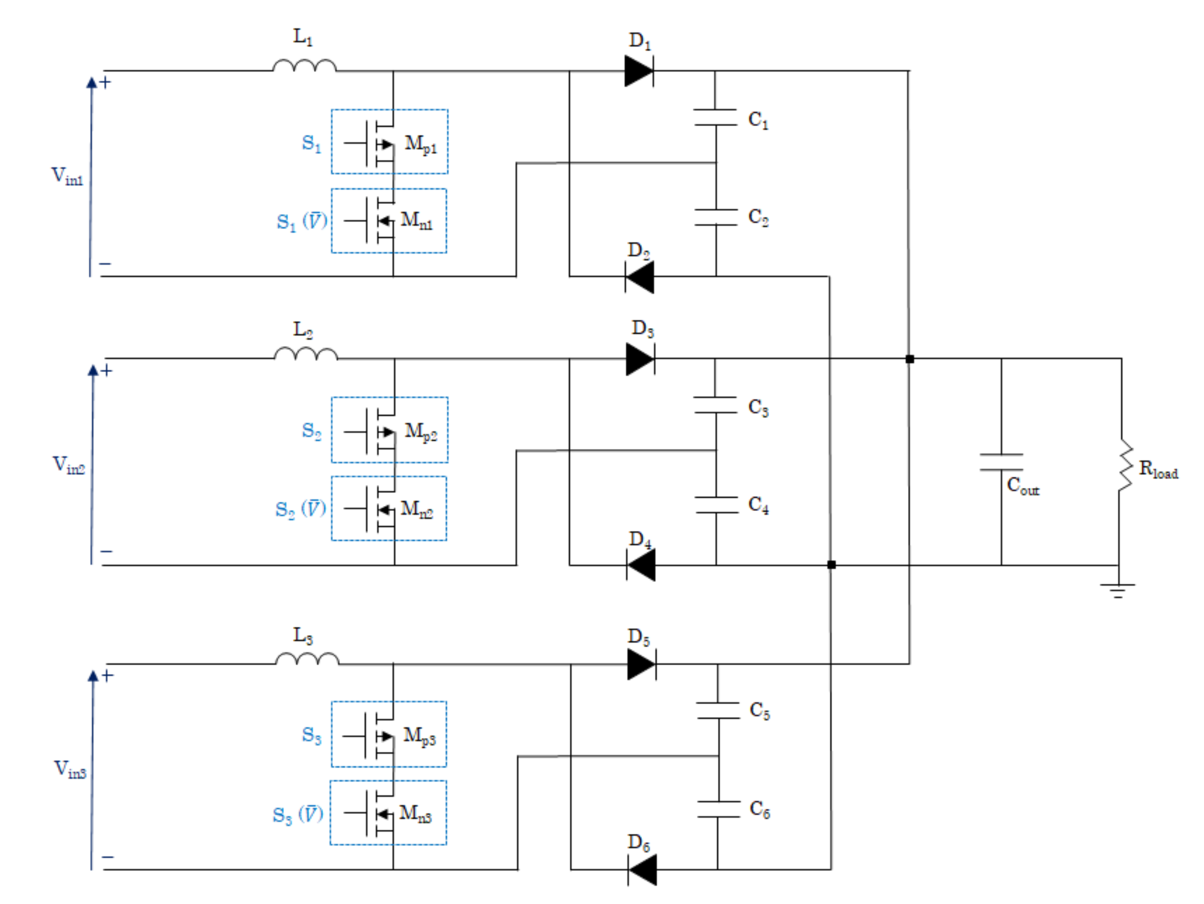
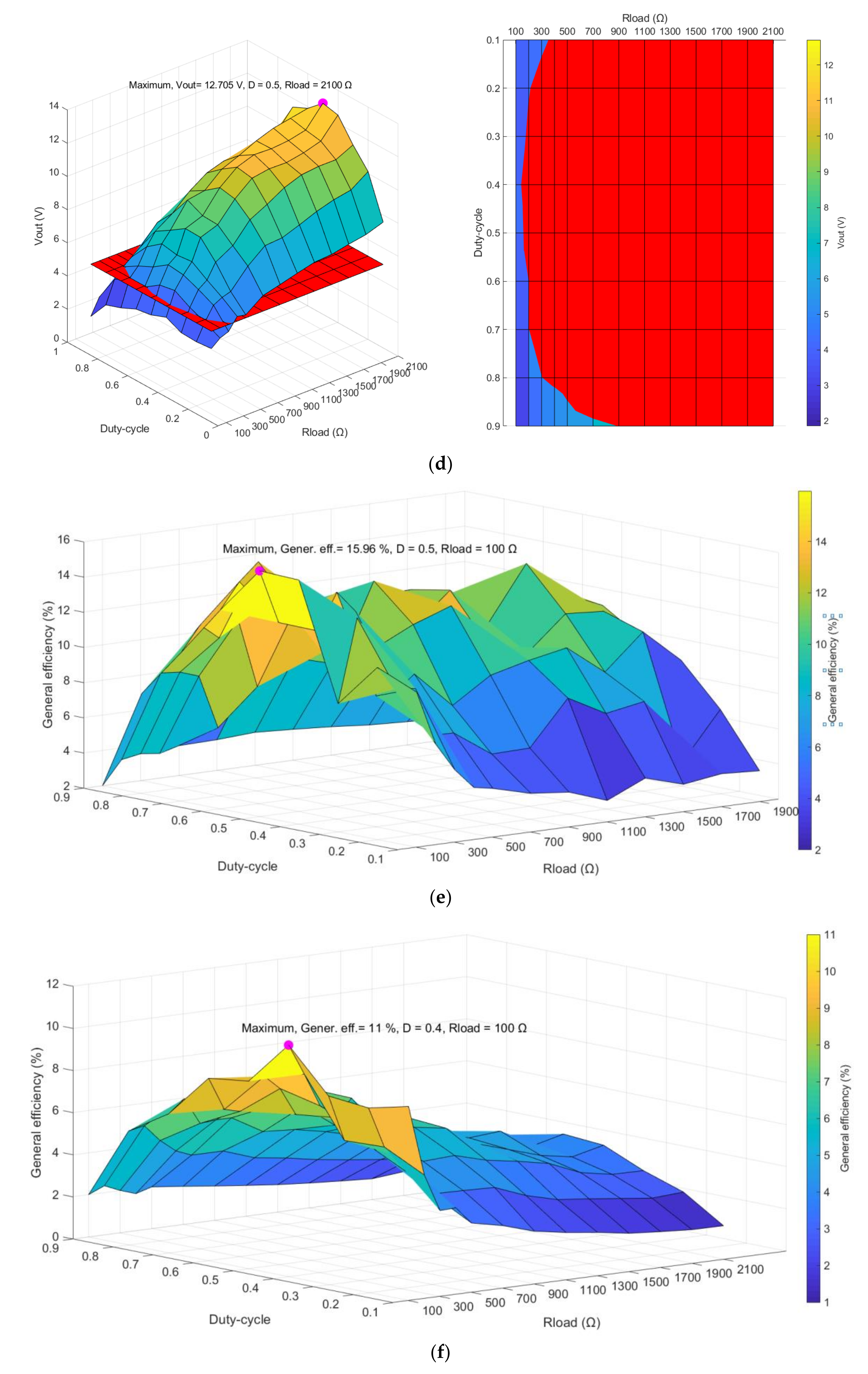
4.1.3. Split-N and Split-NP Topologies
- Split topology with N-type MOSFETs
- Split topology with N and P-type MOSFETs
Split Topology with N-Type MOSFETs
Split Topology with N and P-Type MOSFETs
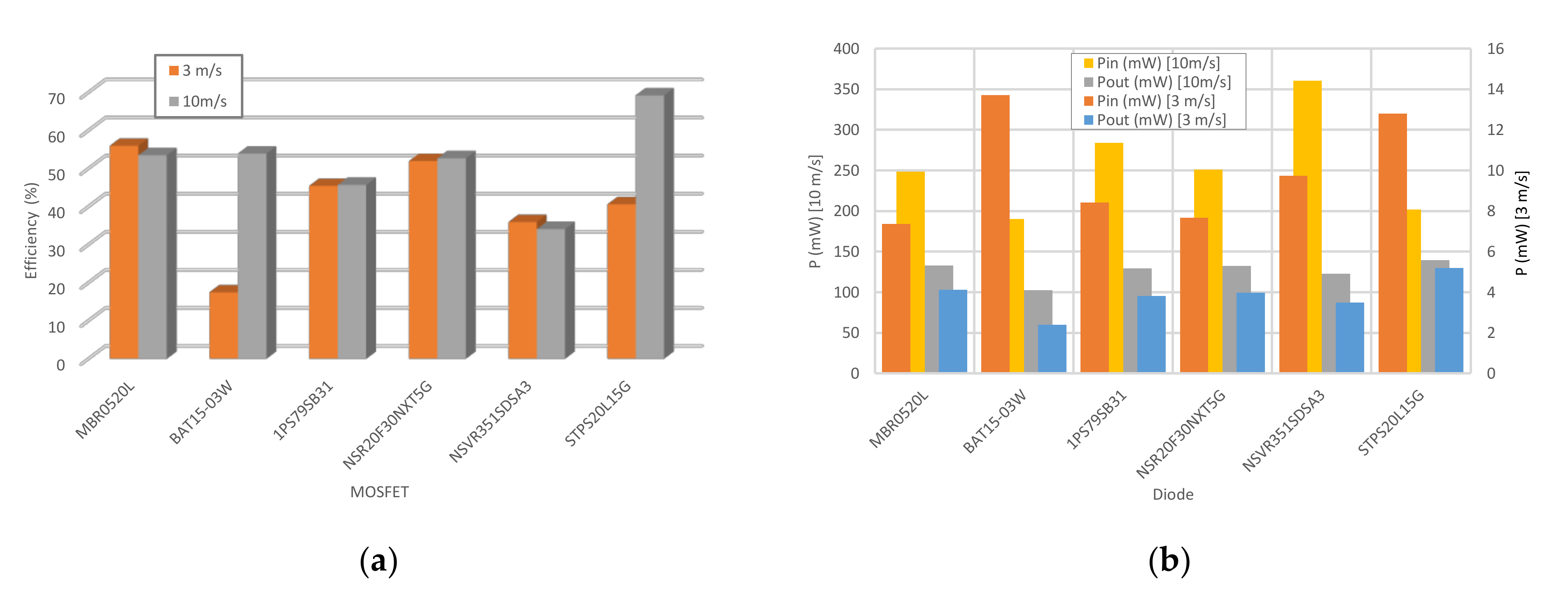
4.2. Diode Selection
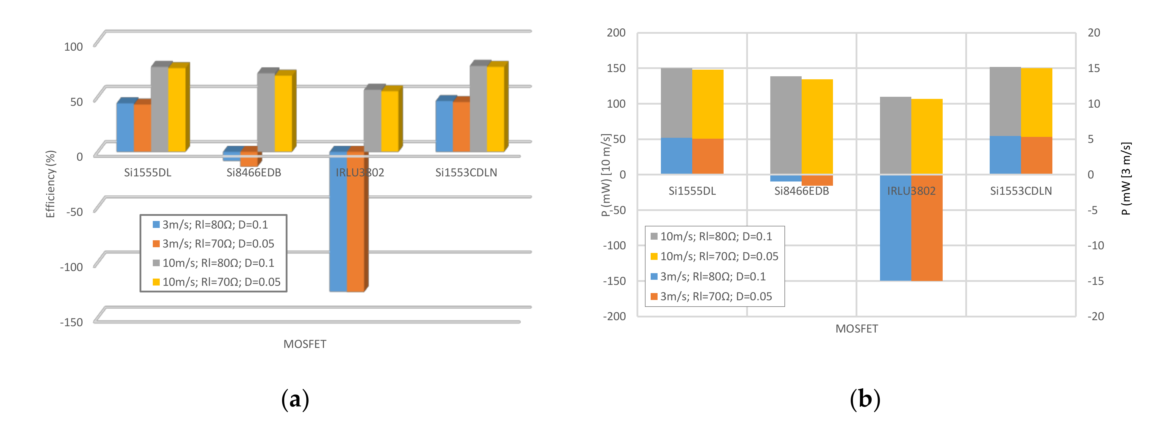
4.3. MOSFET Selection
4.4. Architectures: Evaluation and Selection
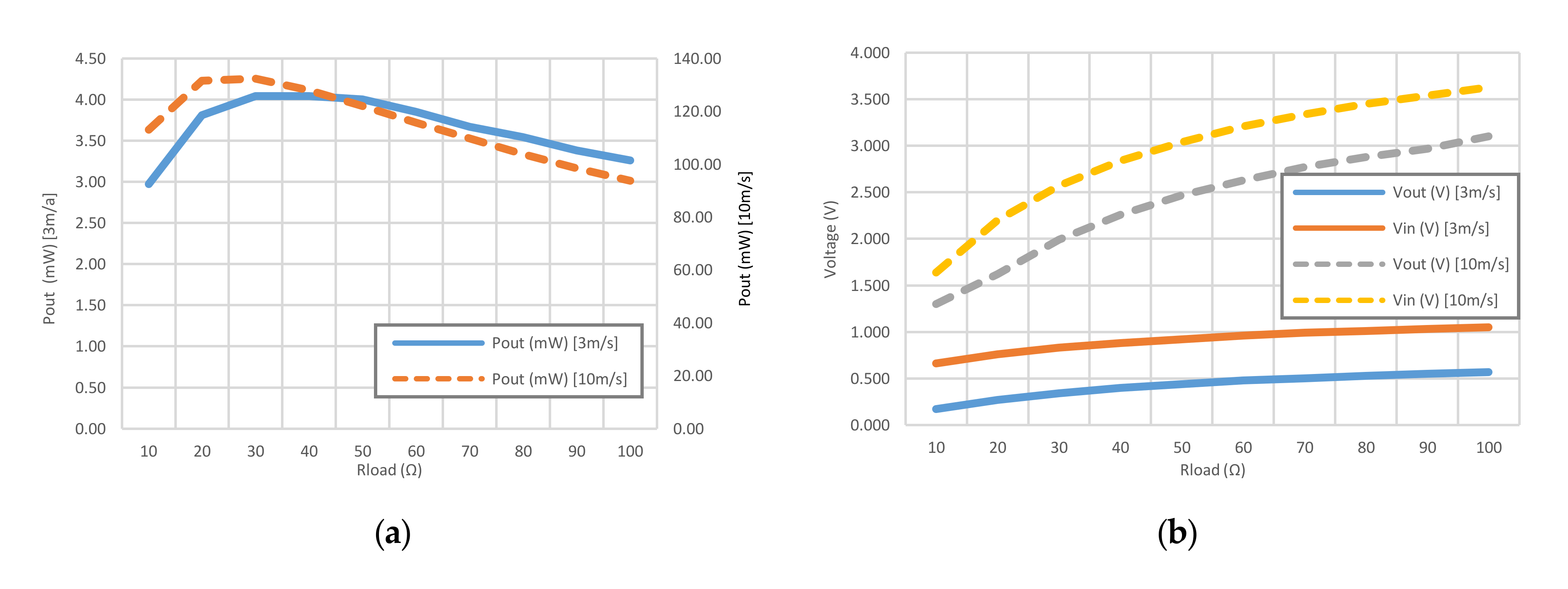
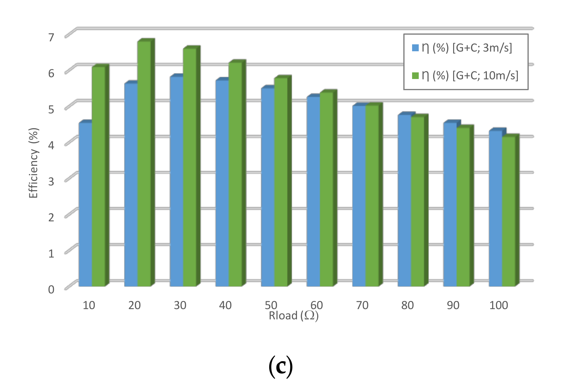
4.4.1. Three-Phase Diode Bridge Rectifier
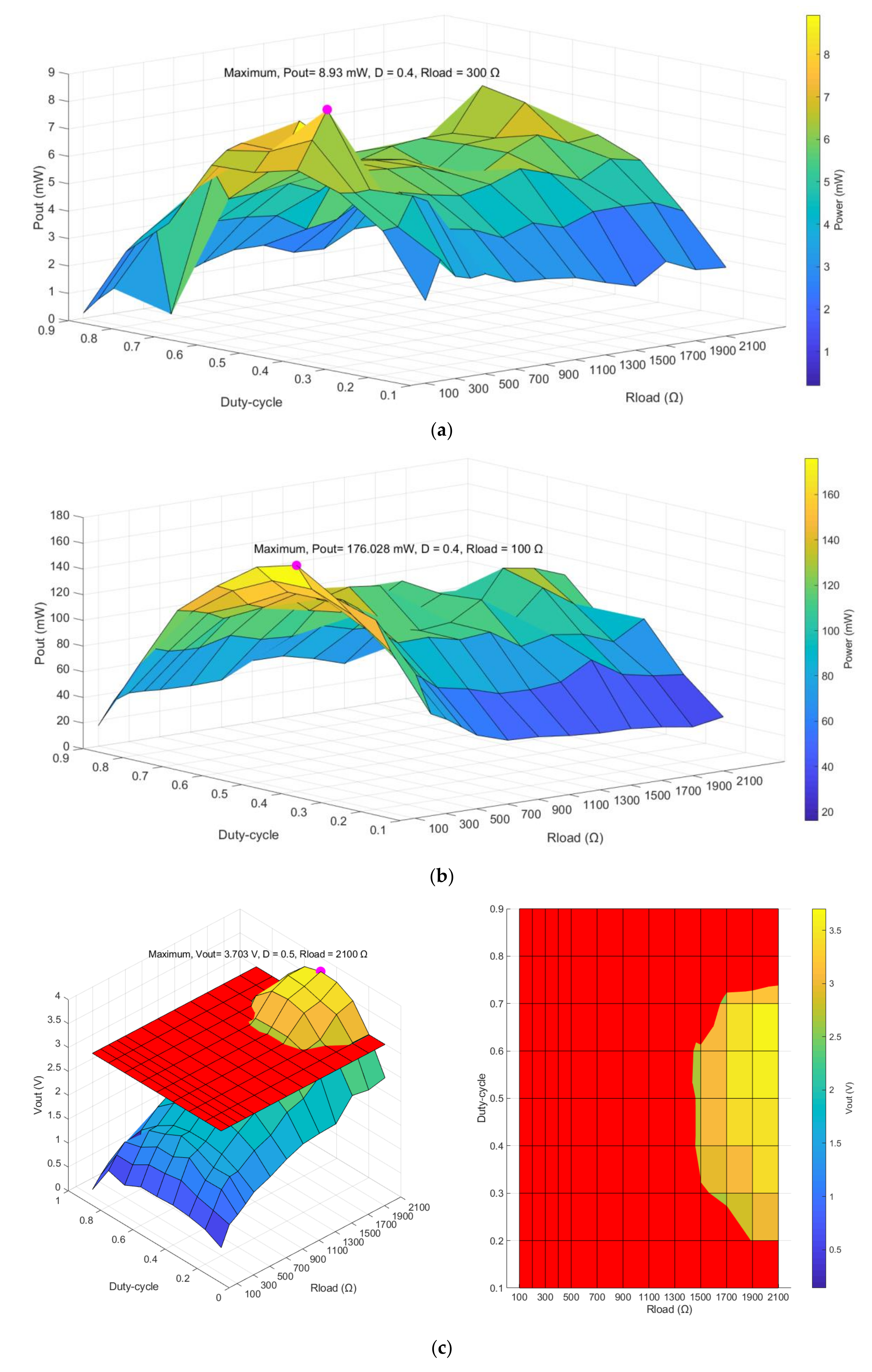
4.4.2. Secondary Side Diode-Based Topology
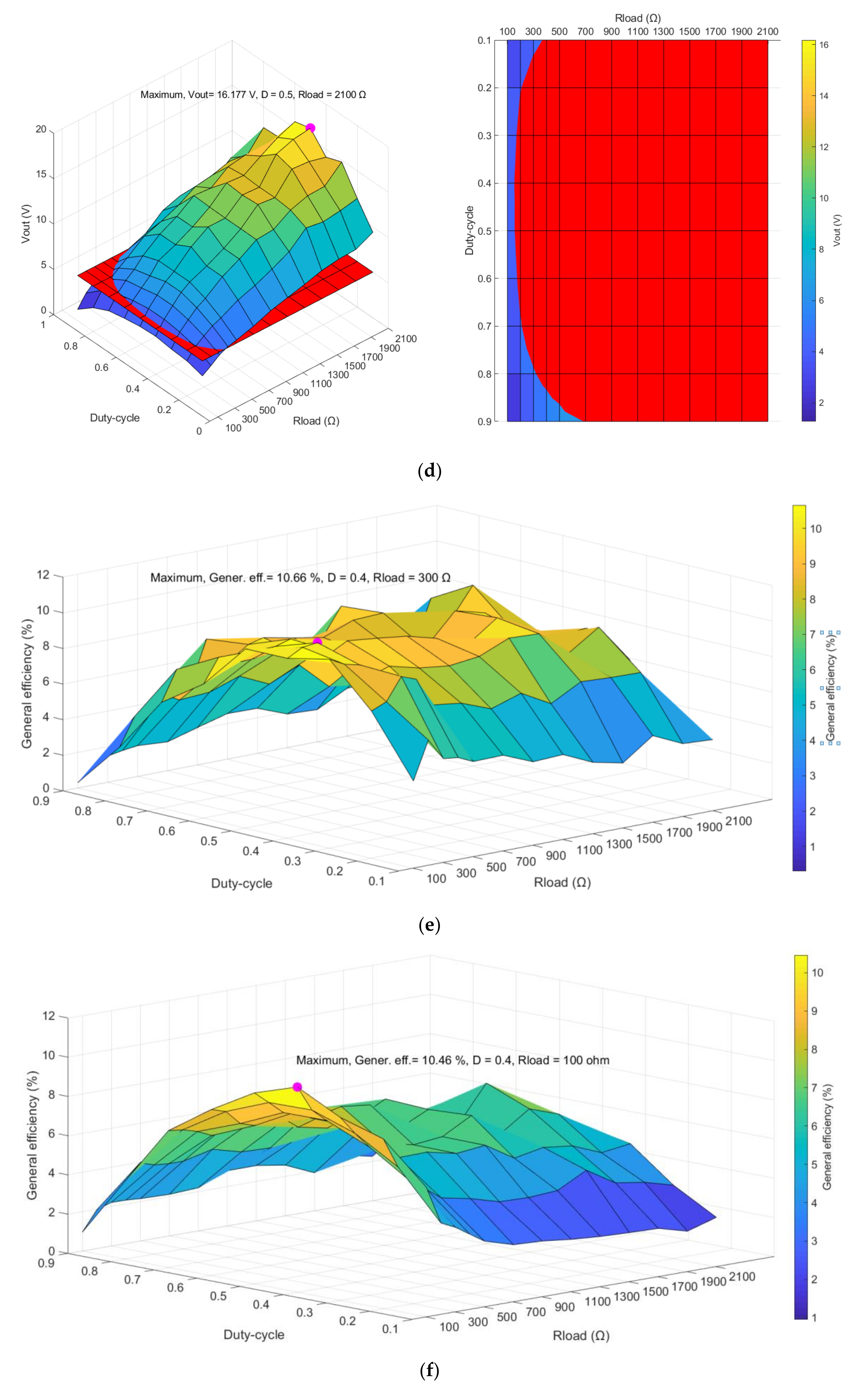
4.4.3. Split Capacitor Topology
Split Topology with N-Type MOSFETs
Split Topology with N and P-Type MOSFETs
4.4.4. Summary of Results and Circuit Selection
5. Application Examples
6. Conclusions
Author Contributions
Funding
Acknowledgments
Conflicts of Interest
References
- Perera, C.; Liu, C.H.; Jayawardena, S.; Chen, M. A Survey on Internet of Things From Industrial Market Perspective. IEEE Access 2015, 2, 1660–1679. [Google Scholar] [CrossRef]
- Wan, J.; Tang, S.; Hua, Q.; Li, D.; Liu, C.; Lloret, J.; Hua, Q. Context-Aware Cloud Robotics for Material Handling in Cognitive Industrial Internet of Things. IEEE Internet Things J. 2018, 5, 2272–2281. [Google Scholar] [CrossRef]
- Lydon, B. Industry 4.0 for Process Automation—Process Sensors 4.0 Roadmap. May 2016. Available online: https://www.automation.com/automation-news/article/industry-40-for-process-automation-process-sensors-40-roadmap (accessed on 1 September 2020).
- O’Mathúna, C.; O’Donnell, T.; Martinez-Catala, R.V.; Rohan, J.F.; O’Flynn, B. Energy scavenging for long-term deployable wireless sensor networks. Talanta Int. J. Pure Appl. Anal. Chem. 2008, 75, 613–623. [Google Scholar]
- Morkevicius, A.; Bisikirskiene, L.; Bleakley, G. Using a Systems of Systems Modeling Approach for Developing Industrial Internet of Things applications. In Proceedings of the 2017 12th System of Systems Engineering Conference (SoSE), Waikoloa, HI, USA, 18–21 June 2017; Institute of Electrical and Electronics Engineers (IEEE): Piscataway, NJ, USA, 2017; pp. 1–6. [Google Scholar]
- Chu, S.; Cui, Y.; Liu, N. The path towards sustainable energy. Nat. Mater. 2016, 16, 16–22. [Google Scholar] [CrossRef]
- Charter, M. Designing for the Circular Economy; Informa UK Limited; Routledge (Taylor&Francis Group): London, UK, 2018. [Google Scholar]
- Zorzi, M.; Gluhak, A.; Lange, S.; Bassi, A. From today’s INTRAnet of things to a future INTERnet of things: A wireless- and mobility-related view. IEEE Wirel. Commun. 2010, 17, 44–51. [Google Scholar] [CrossRef]
- Clifford, G. Energy Harvesting: How We’ll Build the Internet of Perpetual Things. Jabil. Available online: https://www.jabil.com/dam/jcr:3263191a-2168-4ead-be7d-513a994ebf4c/white-paper-energy-harvesting-how-we-will-build-the-internet-of-perpetual-things.pdf (accessed on 1 September 2020).
- Gungor, V.C.; Hancke, G. Industrial Wireless Sensor Networks: Challenges, Design Principles, and Technical Approaches. IEEE Trans. Ind. Electron. 2009, 56, 4258–4265. [Google Scholar] [CrossRef] [Green Version]
- Webster, J.G.; Eren, H. Measurement, Instrumentation, and Sensors Handbook: Spatial, Mechanical, Thermal, and Radiation Measurement, 2nd ed.; CRC Press: Boca Raton, FL, USA, 2014. [Google Scholar]
- Tan, Y.K.; Panda, S.K. Review of Energy Harvesting Technologies for Sustainable Wireless Sensor Network (WSN) 2010. Available online: https://www.intechopen.com/books/sustainable-wireless-sensor-networks/review-of-energy-harvesting-technologies-for-sustainable-wsn (accessed on 1 September 2020).
- Spies, P.; Pollak, M.; Mateu, L. Handbook of Energy Harvesting Power Supplies and Applications; Pan Stanford Publishing: Singapore, 2015. [Google Scholar]
- Munir, B.; Dyo, V. On the Impact of Mobility on Battery-Less RF Energy Harvesting System Performance. Sensors 2018, 18, 3597. [Google Scholar] [CrossRef] [PubMed] [Green Version]
- Vracar, L.; Prijic, A.; Nesic, D.; Dević, S.; Prijic, Z. Photovoltaic Energy Harvesting Wireless Sensor Node for Telemetry Applications Optimized for Low Illumination Levels. Electronics 2016, 5, 26. [Google Scholar] [CrossRef] [Green Version]
- Zhao, L.; Yang, Y. Toward Small-Scale Wind Energy Harvesting: Design, Enhancement, Performance Comparison, and Applicability. Shock. Vib. 2017, 2017, 1–31. [Google Scholar] [CrossRef]
- Nabavi, S.; Zhang, L. Portable Wind Energy Harvesters for Low-Power Applications: A Survey. Sensors 2016, 16, 1101. [Google Scholar] [CrossRef] [Green Version]
- Aljadiri, R.T.; Taha, L.Y.; Ivey, P. Wind energy harvesting systems: A better understanding of their sustainability. In Proceedings of the 2017 3rd International Conference on Control, Automation and Robotics (ICCAR); Institute of Electrical and Electronics Engineers (IEEE), Nagoya, Japan, 22–24 April 2017; pp. 582–587. [Google Scholar]
- Perez, M.; Boisseau, S.; Gasnier, P.; Willemin, J.; Geißler, M.; Reboud, J.L. A cm scale electret-based electrostatic wind turbine for low-speed energy harvesting applications. Smart Mater. Struct. 2016, 25, 45015. [Google Scholar] [CrossRef]
- Bi, M.; Wu, Z.; Wang, S.; Cao, Z.; Cheng, Y.; Ma, X.; Ye, X. Optimization of structural parameters for rotary freestanding-electret generators and wind energy harvesting. Nano Energy 2020, 75, 1–11. [Google Scholar] [CrossRef]
- Elahi, H.; Eugeni, M.; Gaudenzi, P. A Review on Mechanisms for Piezoelectric-Based Energy Harvesters. Energies 2018, 11, 1850. [Google Scholar] [CrossRef] [Green Version]
- Zhang, J.; Fang, Z.; Shu, C.; Zhang, J.; Zhang, Q.; Li, C. A rotational piezoelectric energy harvester for efficient wind energy harvesting. Sens. Actuators A Phys. 2017, 262, 123–129. [Google Scholar] [CrossRef]
- Wang, X.; Liang, X.; Hao, Z.; Du, H.; Zhang, N.; Qian, M. Comparison of electromagnetic and piezoelectric vibration energy harvesters with different interface circuits. Mech. Syst. Signal Process. 2016, 72, 906–924. [Google Scholar] [CrossRef]
- Javed, U.; Abdelkefi, A. Characteristics and comparative analysis of piezoelectric-electromagnetic energy harvesters from vortex-induced oscillations. Nonlinear Dyn. 2019, 95, 3309–3333. [Google Scholar] [CrossRef]
- Dell’Anna, F.G.; Dong, T.; Li, P.; Wen, Y.; Yang, Z.; Casu, M.R.; Azadmehr, M.; Berg, Y.; Yumei, W. State-of-the-Art Power Management Circuits for Piezoelectric Energy Harvesters. IEEE Circuits Syst. Mag. 2018, 18, 27–48. [Google Scholar] [CrossRef]
- Jung, H.J.; Nezami, S.; Lee, S. Power Supply Switch Circuit for Intermittent Energy Harvesting. Electronics 2019, 8, 1446. [Google Scholar] [CrossRef] [Green Version]
- Romani, A.; Filippi, M.; Tartagni, M. Micropower Design of a Fully Autonomous Energy Harvesting Circuit for Arrays of Piezoelectric Transducers. IEEE Trans. Power Electron. 2013, 29, 729–739. [Google Scholar] [CrossRef]
- Choetchai, P.; Thanachayanont, A. A Self-starting AC-to-DC Step-up Converter for Energy Harvesting Applications. Procedia Comput. Sci. 2016, 86, 144–147. [Google Scholar] [CrossRef] [Green Version]
- Pozo, B.; Serras, A.; Fernández de Gorostiza, E. «Mini-Tubine» España. Internacional Patente ES2667562 (A1); WO2018087174 (A1), 13 February 2019. [Google Scholar]
- Ibrahim, B.K. Utilization of wind energy in space heating and cooling with hybrid HVAC systems and heat pumps. Energy Build 1999, 30, 147–153. [Google Scholar]
- Heier, S. Wind Power [a review of Grid Integration of Wind Energy Conversion Systems (S. Heier; 2006); book review]. IEEE Power Energy Mag. 2008, 6, 95–97. [Google Scholar] [CrossRef]
- Calderaro, V.; Galdi, V.; Piccolo, A.; Siano, P. A fuzzy controller for maximum energy extraction from variable speed wind power generation systems. Electr. Power Syst. Res. 2008, 78, 1109–1118. [Google Scholar] [CrossRef]
- Sengupta, A.; Verma, M.P. An analytical expression for the power coefficient of an ideal horizontal-axis wind turbine. Int. J. Energy Res. 1992, 16, 453–455. [Google Scholar] [CrossRef]
- Slootweg, J.; Polinder, H.; Kling, W.L. Representing wind turbine electrical generating systems in fundamental frequency simulations. IEEE Trans. Energy Convers. 2003, 18, 516–524. [Google Scholar] [CrossRef] [Green Version]
- Borowy, B.; Salameh, Z. Methodology for optimally sizing the combination of a battery bank and PV array in a wind/PV hybrid system. IEEE Trans. Energy Convers. 1996, 11, 367–375. [Google Scholar] [CrossRef]
- Hardik, P.; Sanat, D. Performance Prediction of Horizontal Axis Wind Turbine Blade. Int. J. Innov. Res. Sci. Eng. Technol. 2013, 2, 1401–1406. [Google Scholar]
- Pozo, B. Double Smart Energy Harvesting System for Self-Powered Industrial IOT. 2018. Available online: https://www.educacion.gob.es/teseo/mostrarRef.do?ref=444036 (accessed on 1 September 2020).
- Carli, D.; Brunelli, D.; Bertozzi, D.; Benini, L. A high-efficiency wind-flow energy harvester using micro turbine. SPEEDAM 2010 2010, 778–783. [Google Scholar]
- Zakaria, M.Y.; Pereira, D.A.; Hajj, M.R. Experimental investigation and performance modeling of centimeter-scale micro-wind turbine energy harvesters. J. Wind. Eng. Ind. Aerodyn. 2015, 147, 58–65. [Google Scholar] [CrossRef]
- Rancourt, D.A.T.; Fréchette, L.G. Evaluation of Centimeter-Scale Micro Wind Mills: Aerodynamics and Electromagnetic Power Generation. In Proceedings of the 7th international Workshop on Micro and Nanotechnology for Power Generation & Energy Conversion App’s (PowerMEMS ’07), Freiburg, Germany, 27–29 November 2007. [Google Scholar]
- Xu, F.; Yuan, F.-G.; Liu, L.; Hu, J.; Qiu, Y. Performance Prediction and Demonstration of a Miniature Horizontal Axis Wind Turbine. J. Energy Eng. 2013, 139, 143–152. [Google Scholar] [CrossRef]
- Dwari, S.; Parsa, L. Low Voltage Energy Harvesting Systems Using Coil Inductance of Electromagnetic Microgenerators. In Proceedings of the 2009 Twenty-Fourth Annual IEEE Applied Power Electronics Conference and Exposition, Washington, DC, USA, 15–19 February 2009; Institute of Electrical and Electronics Engineers (IEEE): Piscataway, NJ, USA, 2009; pp. 1145–1150. [Google Scholar]
- Dayal, R.; Dwari, S.; Parsa, L. Design and Implementation of a Direct AC–DC Boost Converter for Low-Voltage Energy Harvesting. IEEE Trans. Ind. Electron. 2010, 58, 2387–2396. [Google Scholar] [CrossRef]
- LTspice—Analog Devices. Available online: http://www.analog.com/en/design-center/design-tools-and-calculators/ltspice-simulator.html# (accessed on 15 December 2019).
- PSIM—PowerSIM. Available online: https://powersimtech.com/products/psim/ (accessed on 1 September 2020).
- Dwari, S.; Dayal, R.; Parsa, L.; Salama, K.N. Efficient direct ac-to-dc converters for vibration-based low voltage energy harvesting. In Proceedings of the 2008 34th Annual Conference of IEEE Industrial Electronics, Orlando, FL, USA, 10–13 November 2008; Institute of Electrical and Electronics Engineers (IEEE): Piscataway, NJ, USA, 2008; pp. 2320–2325. [Google Scholar]
- Dwari, S.; Dayal, R.; Parsa, L. A Novel direct AC/DC converter for efficient low voltage energy harvesting. In Proceedings of the 2008 34th Annual Conference of IEEE Industrial Electronics, Orlando, FL, USA, 10–13 November 2008; Institute of Electrical and Electronics Engineers (IEEE): Piscataway, NJ, USA, 2008; pp. 484–488. [Google Scholar]
- Dwari, S.; Parsa, L. An Efficient AC–DC Step-Up Converter for Low-Voltage Energy Harvesting. IEEE Trans. Power Electron. 2010, 25, 2188–2199. [Google Scholar] [CrossRef]
- MBR0520L. 2014. Available online: http://www.onsemi.com/pub/Collateral/MBR0520L-D.pdf (accessed on 1 September 2020).
- BAT15-03W. 2018. Available online: http://www.infineon.com/dgdl/Infineon-BAT15-03W-DS-v01_00-EN.pdf?fileId=5546d46265f064ff01663896078c4e80 (accessed on 1 September 2020).
- 1PS79SB31. 11 January 2002. Available online: http://assets.nexperia.com/documents/data-sheet/1PS79SB31.pdf (accessed on 1 September 2020).
- NSR20F30NXT5G. 2013. Available online: http://www.onsemi.com/pub/Collateral/NSR20F30-D.PDF (accessed on 1 September 2020).
- NSVR351SDSA3. 2018. Available online: http://www.onsemi.com/pub/Collateral/NSVR351SDSA3-D.PDF (accessed on 1 September 2020).
- STPS20L15. 2016. Available online: http://www.st.com/resource/en/datasheet/stps20l15.pdf (accessed on 1 September 2020).
- Si1555DL. 2017. Available online: http://www.vishay.com/docs/71079/71079.pdf (accessed on 1 September 2020).
- Si8466EDB. 2017. Available online: http://www.vishay.com/docs/63683/si8466edb.pdf (accessed on 1 September 2020).
- IRLR3802. 2011. Available online: https://www.infineon.com/dgdl/irlr3802pbf.pdf?fileId=5546d462533600a40153566d742526b5 (accessed on 1 September 2020).
- Si1553CDL. 2017. Available online: http://www.vishay.com/docs/67693/si1553cdl.pdf (accessed on 1 September 2020).
- Li, P.; Wen, Y.; Yin, W.; Wu, H. An Upconversion Management Circuit for Low-Frequency Vibrating Energy Harvesting. IEEE Trans. Ind. Electron. 2013, 61, 3349–3358. [Google Scholar] [CrossRef]
- Yu, H.; Zhou, J.; Deng, L.; Wen, Z. A Vibration-Based MEMS Piezoelectric Energy Harvester and Power Conditioning Circuit. Sensors 2014, 14, 3323–3341. [Google Scholar] [CrossRef] [PubMed]


| System Values | |
|---|---|
| ρ | 1.225 |
| A_harvester | 0.00045 |
| r_harvester | 0.016 |
| r_rotor | 0.00355 |
| length_blades | 0.01476 |
| θ | 34.45 |
| weight | 0.0032 |
| length_swept | 0.024 |
| A_small_pipe | 3.31 × 10⁻⁵ |
| A_big_pipe | 0.000829 |
| Cp Coefficient | c1 | c2 | c3 | c4 | c5 | c6 | c7 | c8 | c9 |
|---|---|---|---|---|---|---|---|---|---|
| CSMWT | 0.6 | 160 | 0.93 | 0 | 0 | 9.3 | 9.8 | 0.037 | 0 |
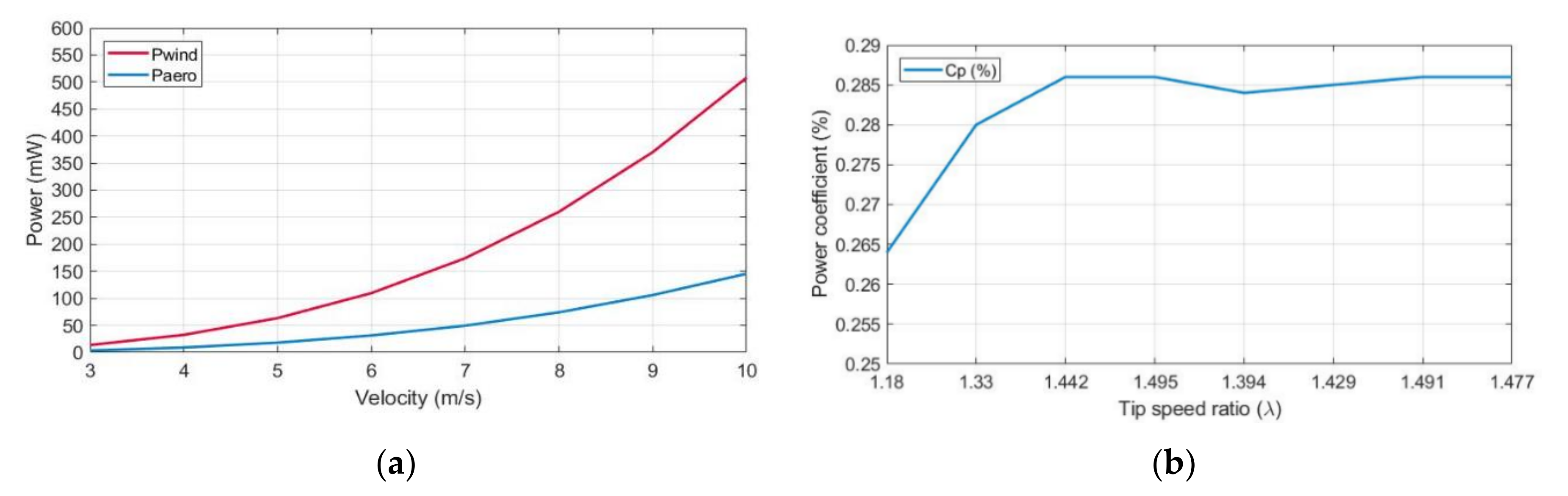
| ω (rpm) | ω (rad/s) | Velocity (m/s) | Pwind (mW) | Paero (mW) | Cp(λ,θ) | λi | λ | Q (m3/s) |
|---|---|---|---|---|---|---|---|---|
| 9495 | 997 | 3 | 13.719 | 3.622 | 0.264 | 2.454 | 1.180 | 0.002 |
| 14,271 | 1498 | 4 | 32.518 | 9.104 | 0.280 | 2.605 | 1.330 | 0.003 |
| 19,344 | 2031 | 5 | 63.513 | 18.147 | 0.286 | 2.717 | 1.442 | 0.004 |
| 24,057 | 2526 | 6 | 109.750 | 31.443 | 0.286 | 2.769 | 1.495 | 0.005 |
| 26,180 | 2749 | 7 | 174.279 | 49.484 | 0.284 | 2.669 | 1.394 | 0.006 |
| 30,666 | 3219 | 8 | 260.148 | 74.230 | 0.285 | 2.704 | 1.429 | 0.007 |
| 35,995 | 3779 | 9 | 370.405 | 106.114 | 0.286 | 2.765 | 1.491 | 0.007 |
| 39,616 | 4159 | 10 | 508.101 | 145.507 | 0.286 | 2.751 | 1.477 | 0.008 |
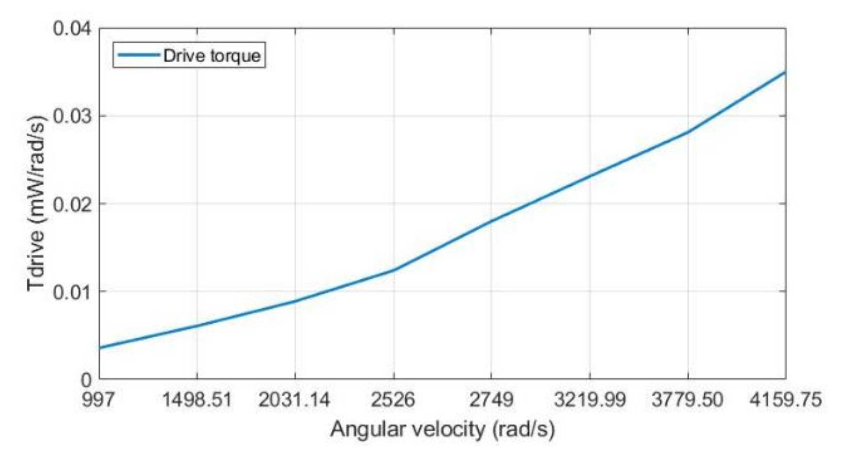
| Angular Velocity (rad/s) | Tdrive (mW/rad/s) |
|---|---|
| 997 | 0.0036 |
| 1498.51 | 0.0061 |
| 2031.14 | 0.0089 |
| 2526 | 0.0124 |
| 2749 | 0.0180 |
| 3219.99 | 0.0231 |
| 3779.50 | 0.0281 |
| 4159.75 | 0.0350 |
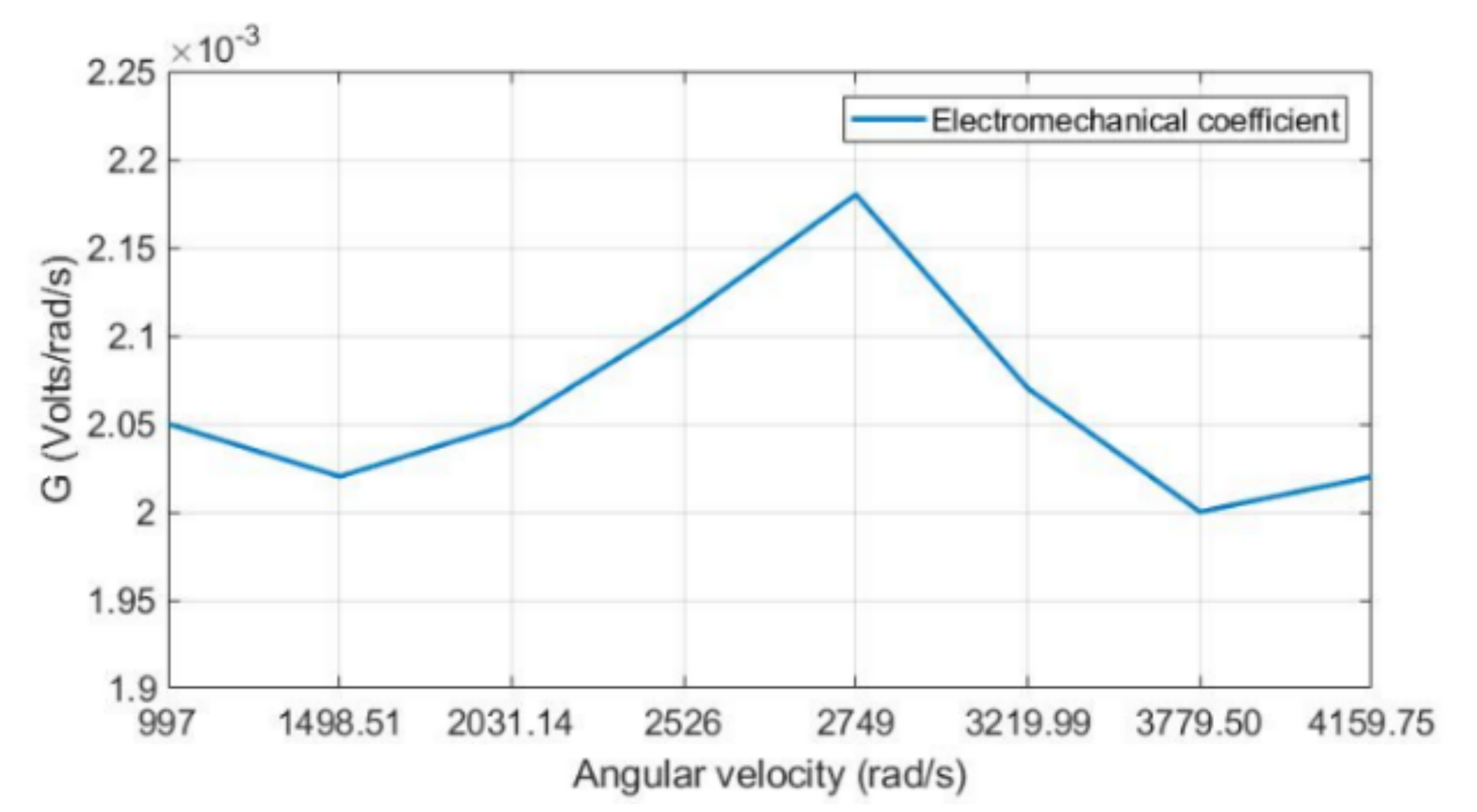
| Velocity (m/s) | Voltage (V) | ω (rad/s) | G (Volt/rad/s) |
|---|---|---|---|
| 3 | 2.05 | 997 | 0.00205 |
| 4 | 3.02 | 1498.51 | 0.00202 |
| 5 | 4.17 | 2031.14 | 0.00205 |
| 6 | 5.32 | 2526 | 0.00211 |
| 7 | 5.98 | 2749 | 0.00218 |
| 8 | 6.66 | 3219.99 | 0.00207 |
| 9 | 7.57 | 3779.50 | 0.00200 |
| 10 | 8.38 | 4159.75 | 0.00202 |
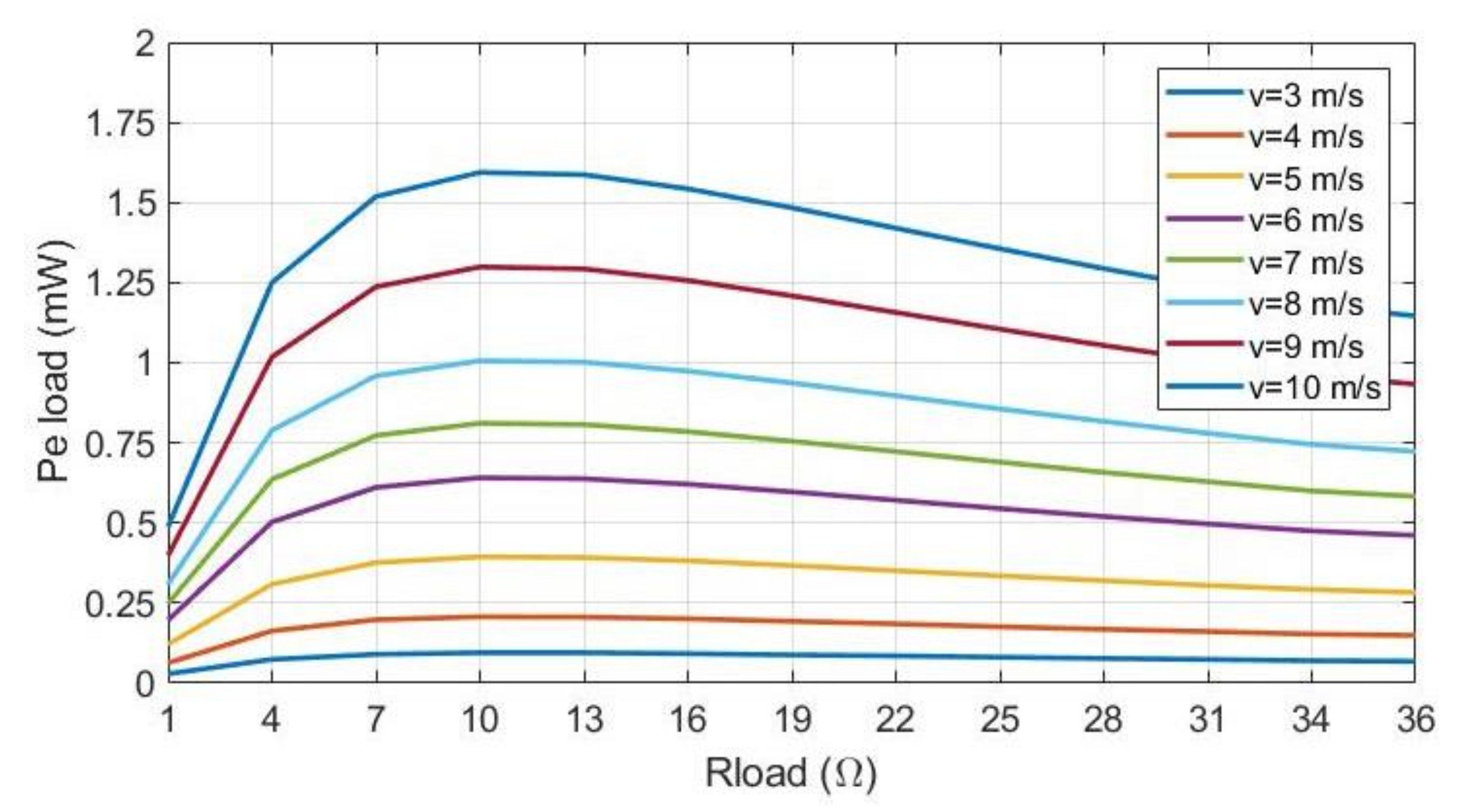
| Pe_load (mW) | |||||||||||||
|---|---|---|---|---|---|---|---|---|---|---|---|---|---|
| Velocity (m/s) | 1 Ω | 4 Ω | 7 Ω | 10 Ω | 13 Ω | 16 Ω | 19 Ω | 22 Ω | 25 Ω | 28 Ω | 31 Ω | 34 Ω | 36 Ω |
| 3 | 0.029 | 0.074 | 0.090 | 0.095 | 0.095 | 0.092 | 0.088 | 0.085 | 0.081 | 0.077 | 0.074 | 0.070 | 0.068 |
| 4 | 0.063 | 0.163 | 0.198 | 0.207 | 0.206 | 0.201 | 0.193 | 0.185 | 0.176 | 0.168 | 0.161 | 0.153 | 0.149 |
| 5 | 0.121 | 0.309 | 0.376 | 0.394 | 0.392 | 0.382 | 0.367 | 0.351 | 0.335 | 0.320 | 0.305 | 0.292 | 0.283 |
| 6 | 0.196 | 0.503 | 0.611 | 0.641 | 0.638 | 0.621 | 0.597 | 0.571 | 0.545 | 0.520 | 0.497 | 0.475 | 0.461 |
| 7 | 0.248 | 0.636 | 0.773 | 0.811 | 0.807 | 0.785 | 0.755 | 0.723 | 0.690 | 0.658 | 0.629 | 0.600 | 0.583 |
| 8 | 0.308 | 0.789 | 0.959 | 1.006 | 1.002 | 0.974 | 0.937 | 0.897 | 0.856 | 0.817 | 0.780 | 0.745 | 0.723 |
| 9 | 0.398 | 1.018 | 1.237 | 1.299 | 1.293 | 1.257 | 1.209 | 1.157 | 1.105 | 1.054 | 1.007 | 0.962 | 0.933 |
| 10 | 0.488 | 1.250 | 1.519 | 1.594 | 1.587 | 1.543 | 1.484 | 1.420 | 1.356 | 1.294 | 1.235 | 1.180 | 1.146 |
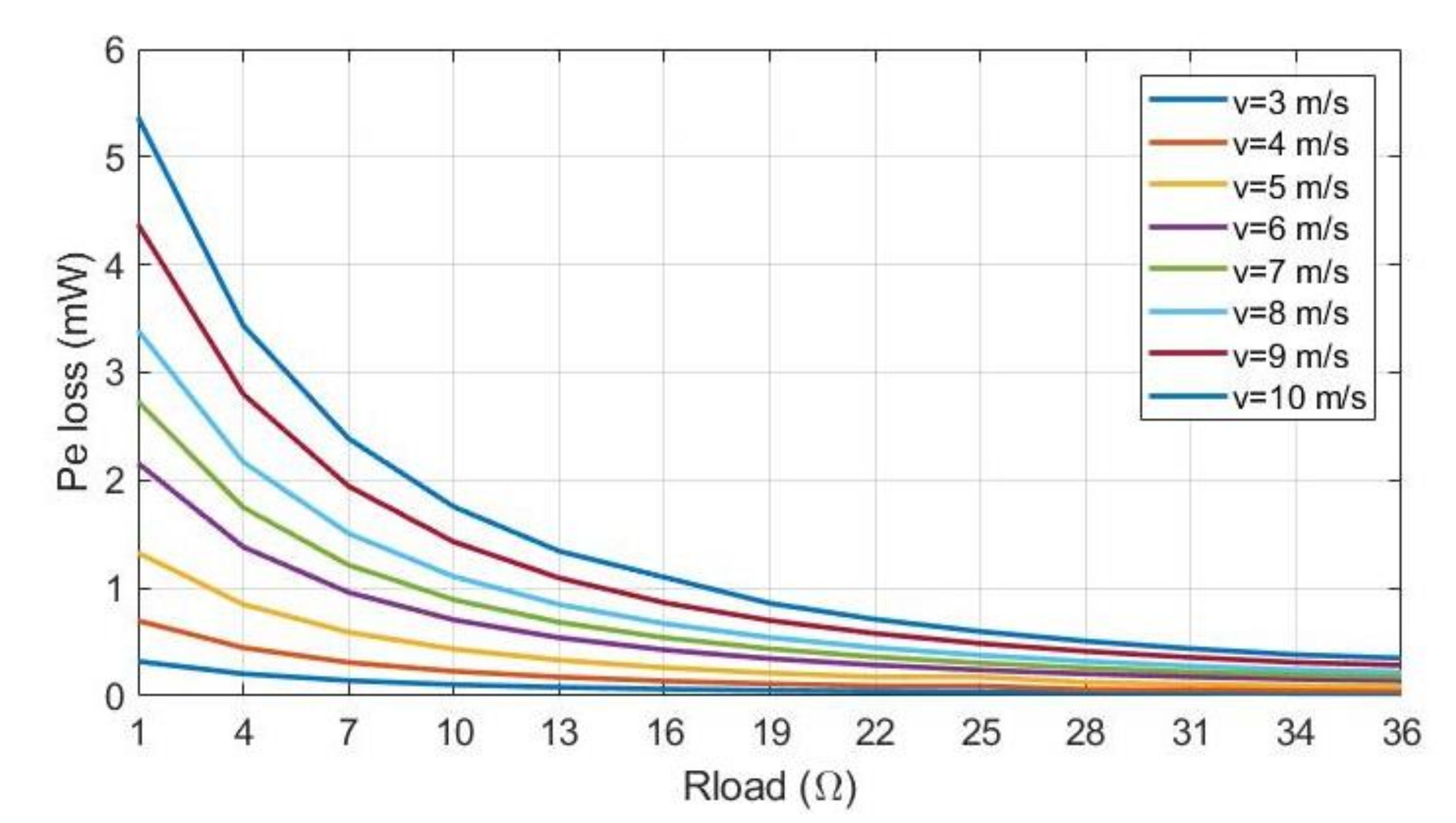
| Pe_loss (mW) | |||||||||||||
|---|---|---|---|---|---|---|---|---|---|---|---|---|---|
| Velocity (m/s) | 1 Ω | 4 Ω | 7 Ω | 10 Ω | 13 Ω | 16 Ω | 19 Ω | 22 Ω | 25 Ω | 28 Ω | 31 Ω | 34 Ω | 36 Ω |
| 3 | 0.320 | 0.205 | 0.142 | 0.104 | 0.080 | 0.063 | 0.051 | 0.042 | 0.036 | 0.030 | 0.026 | 0.023 | 0.021 |
| 4 | 0.698 | 0.447 | 0.310 | 0.228 | 0.175 | 0.138 | 0.112 | 0.092 | 0.092 | 0.06 | 0.057 | 0.050 | 0.046 |
| 5 | 1.328 | 0.850 | 0.590 | 0.434 | 0.332 | 0.262 | 0.212 | 0.176 | 0.176 | 0.126 | 0.108 | 0.094 | 0.087 |
| 6 | 2.160 | 1.382 | 0.960 | 0.705 | 0.540 | 0.427 | 0.346 | 0.286 | 0.240 | 0.204 | 0.176 | 0.154 | 0.141 |
| 7 | 2.732 | 1.748 | 1.214 | 0.892 | 0.683 | 0.540 | 0.437 | 0.361 | 0.304 | 0.259 | 0.223 | 0.194 | 0.178 |
| 8 | 3.390 | 2.170 | 1.507 | 1.107 | 0.848 | 0.670 | 0.542 | 0.448 | 0.377 | 0.321 | 0.277 | 0.241 | 0.221 |
| 9 | 4.375 | 2.800 | 1.945 | 1.429 | 1.094 | 0.864 | 0.700 | 0.579 | 0.486 | 0.414 | 0.357 | 0.311 | 0.285 |
| 10 | 5.370 | 3.437 | 2.387 | 1.754 | 1.343 | 1.1 | 0.859 | 0.710 | 0.597 | 0.508 | 0.438 | 0.382 | 0.350 |
| v = 3 m/s | v = 4 m/s | |||
|---|---|---|---|---|
| Rload (Ω) | 36 | 1 × 10⁶ | 36 | 1 × 10⁶ |
| Voltage (Vpp) | 0.06 | 0.152 | 0.116 | 0.28 |
| Pelectric (mW) | 0.037 | 8.66 × 10⁻⁶ | 0.14 | 2.95 × 10⁻⁵ |
| Pwind (mW) | 13.718 | 32.518 | ||
| Paero (mW) | 0.389 | 0.473 | 1.019 | 1.295 |
| λ | 0.043 | 0.088 | 0.066 | 0.124 |
| Cp(λ,θ) | 0.028 | 0.034 | 0.031 | 0.039 |
| Efficiency (%) | 0.269 | 6.31 × 10⁻⁶ | 0.43 | 9.07 × 10⁻⁵ |
| γ (g/cm3) | A (cm2) | v (cm/s) | Q (cm3/s) | H (mbar) | Wind Power (mW) |
|---|---|---|---|---|---|
| 0.0013 | 8.04 | 300 | 2412 | 20 | 62.712 |
| 0.0013 | 8.04 | 400 | 3216 | 36 | 150.509 |
| 0.0013 | 8.04 | 500 | 4020 | 52 | 271.752 |
| 0.0013 | 8.04 | 600 | 4824 | 91 | 570.679 |
| 0.0013 | 8.04 | 700 | 5628 | 112 | 819.437 |
| 0.0013 | 8.04 | 800 | 6432 | 142 | 1187.347 |
| 0.0013 | 8.04 | 900 | 7236 | 144 | 1354.579 |
| 0.0013 | 8.04 | 1000 | 8040 | 163 | 1703.676 |
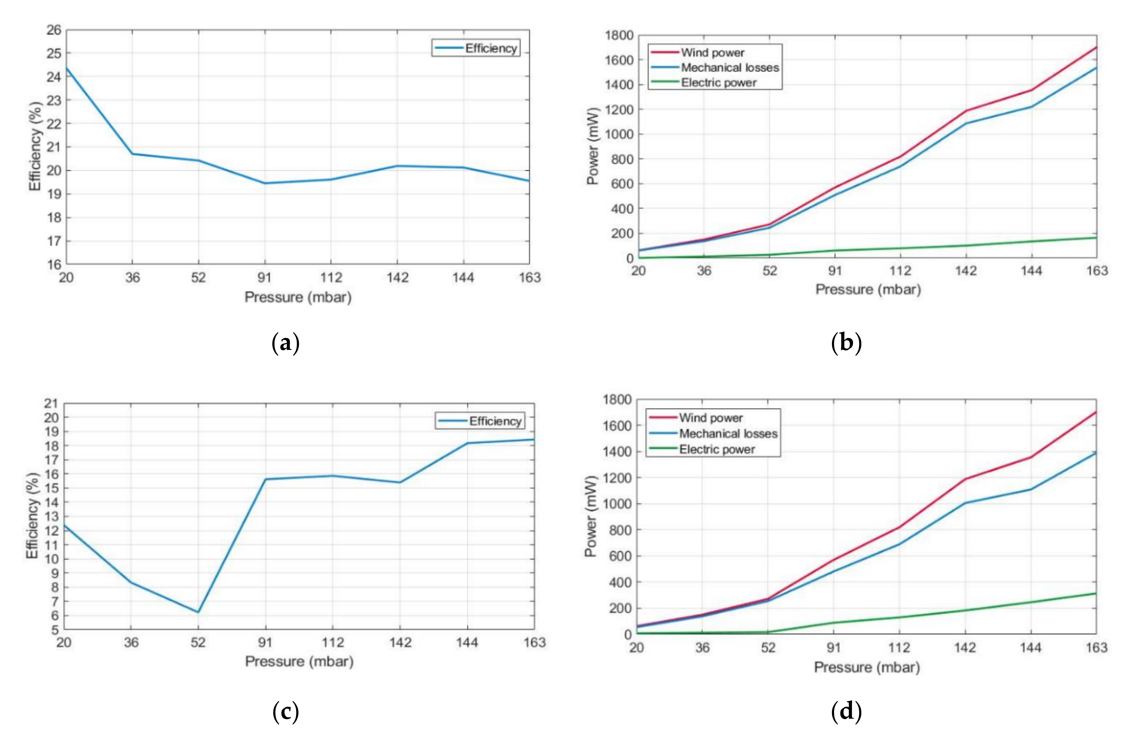
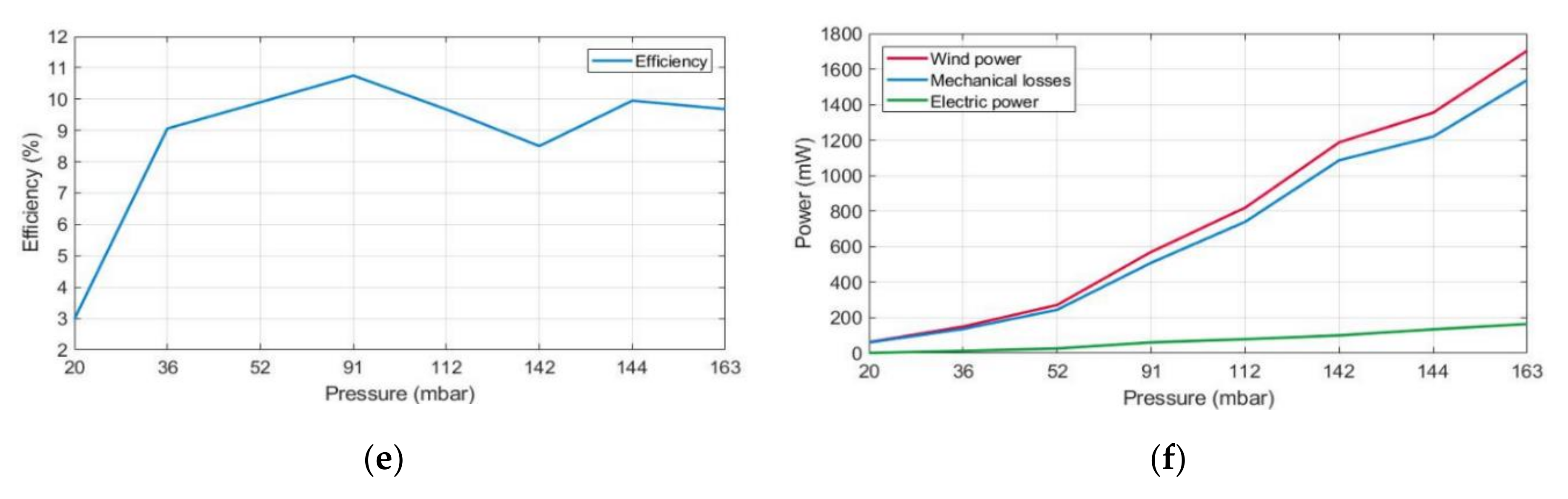
| v (m/s) | Pressure (mbar) | Wind Power (mW) | Rload (Ω) | Elec. Power (mW) | Mech. Losses (mW) | Efficiency (%) |
|---|---|---|---|---|---|---|
| 3 | 20 | 62.712 | 15.284 | 47.428 | 24.37 | |
| 4 | 36 | 150.509 | 31.155 | 119.354 | 20.70 | |
| 5 | 52 | 271.752 | 55.489 | 216.263 | 20.42 | |
| 6 | 91 | 570.679 | 27 | 111.023 | 459.657 | 19.45 |
| 7 | 112 | 819.437 | 160.716 | 658.721 | 19.61 | |
| 8 | 142 | 1187.347 | 239.686 | 947.661 | 20.19 | |
| 9 | 144 | 1354.579 | 272.543 | 1082.036 | 20.12 | |
| 10 | 163 | 1703.676 | 333.146 | 1370.530 | 19.55 | |
| 3 | 20 | 62.712 | 15.284 | 47.428 | 24.37 | |
| 4 | 36 | 150.509 | 31.155 | 119.354 | 20.70 | |
| 5 | 52 | 271.752 | 55.489 | 216.263 | 20.42 | |
| 6 | 91 | 570.679 | 11 | 111.023 | 459.657 | 19.45 |
| 7 | 112 | 819.437 | 160.716 | 658.721 | 19.61 | |
| 8 | 142 | 1187.347 | 239.686 | 947.661 | 20.19 | |
| 9 | 144 | 1354.579 | 272.543 | 1082.036 | 20.12 | |
| 10 | 163 | 1703.676 | 333.146 | 1370.530 | 19.55 | |
| 3 | 20 | 62.712 | 15.284 | 47.428 | 24.37 | |
| 4 | 36 | 150.509 | 31.155 | 119.354 | 20.70 | |
| 5 | 52 | 271.752 | 55.489 | 216.263 | 20.42 | |
| 6 | 91 | 570.679 | 100 | 111.023 | 459.657 | 19.45 |
| 7 | 112 | 819.437 | 160.716 | 658.721 | 19.61 | |
| 8 | 142 | 1187.347 | 239.686 | 947.661 | 20.19 | |
| 9 | 144 | 1354.579 | 272.543 | 1082.036 | 20.12 | |
| 10 | 163 | 1703.676 | 333.146 | 1370.530 | 19.55 |
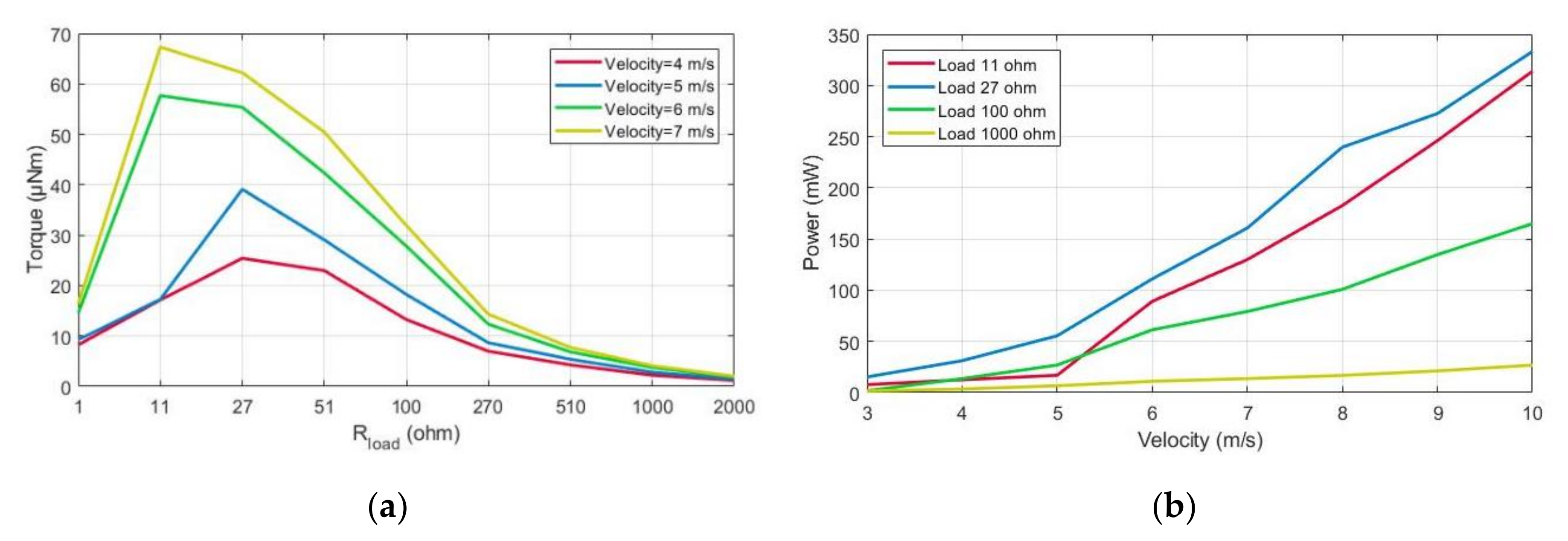
| Torque (µNm) | ||||
|---|---|---|---|---|
| Load (Ω) | Velocity (m/s) | |||
| 4 | 5 | 6 | 7 | |
| 1 | 8.26 | 9.27 | 14.55 | 16.37 |
| 11 | 17.15 | 17.25 | 57.67 | 67.30 |
| 27 | 25.41 | 39.10 | 55.37 | 62.23 |
| 51 | 22.97 | 29.06 | 42.34 | 50.43 |
| 100 | 13.26 | 18.25 | 27.83 | 31.93 |
| 270 | 6.99 | 8.67 | 12.35 | 14.33 |
| 510 | 4.28 | 5.39 | 6.85 | 7.74 |
| 1000 | 2.23 | 2.83 | 3.74 | 4.10 |
| 2000 | 1.20 | 1.46 | 1.86 | 2.02 |
| Power (mW) | ||||
|---|---|---|---|---|
| Velocity (m/s) | Resistor Load (Ω) | |||
| 1 | 27 | 11 | 100 | |
| 3 | 1.61 | 15.28 | 7.77 | 1.87 |
| 4 | 3.45 | 31.16 | 12.54 | 13.64 |
| 5 | 6.72 | 55.49 | 16.93 | 26.91 |
| 6 | 11.04 | 111.02 | 89.15 | 61.34 |
| 7 | 13.68 | 160.72 | 129.94 | 79.25 |
| 8 | 16.80 | 239.69 | 182.70 | 100.87 |
| 9 | 21.21 | 272.54 | 246.13 | 134.79 |
| 10 | 26.86 | 333.15 | 313.92 | 164.98 |
| Ref | Size (mm) | Voltage (V) | Wind Velocity (m/s) | Max Output Power (mW) | Cp (%) | Power Density Per Area (mW × cm2) | Topology |
|---|---|---|---|---|---|---|---|
| [20] | 10 ø | 80 | 2.7 | 18.3 | - | 0.58 | Electrostatic |
| [19] | 40 ø | 450 | 10 | 1.8 | 0.24 | 0.143 | Electrostatic |
| [17] | 161 × 250 | 30 | 5.8 | 53 | - | 0.13 | Piezoelectric |
| [22] | 30 × 12.5 | 14 | 160.2 | 2.56 | - | 0.68 | Piezoelectric |
| [24] | 70 × 20 | 7.86 | 14 | 0.061 | - | 0.004 | Piezoelectric |
| [17] | 490 × 20 | 6 | 7 | 70 | 3.46 | 0.71 | Electromagnetic |
| [39] | 26 ø | 2.2 | 10 | 7 mW | 11 | 1.07 | Electromagnetic |
| [40] | 42 ø | 2.6 | 11.8 | 130 | - | 2.34 | Electromagnetic |
| This work | 32 ø | 2.45 | 10 | 333 | 28 | 10.32 | Electromagnetic |
| Velocity (m/s) | Voltage (V) | ω (rad/s) | G (V/rad/s) |
|---|---|---|---|
| 3 | 2.05 | 997 | 0.00205 |
| 4 | 3.02 | 1498.51 | 0.00202 |
| 5 | 4.17 | 2031.14 | 0.00205 |
| 6 | 5.32 | 2526 | 0.00211 |
| 7 | 5.98 | 2749 | 0.00218 |
| 8 | 6.66 | 3219.99 | 0.00207 |
| 9 | 7.57 | 3779.50 | 0.00200 |
| 10 | 8.38 | 4159.75 | 0.00202 |
| x0 | x2 | δ |
| 0.169 | 0.153 | 0.0215 |
| x0 | x6 | δ |
| 0.169 | 0.129 | 0.0195 |
| x0 | x10 | δ |
| 0.169 | 0.0965 | 0.0243 |
| Rload = 27 Ω | |||||||||
|---|---|---|---|---|---|---|---|---|---|
| v (m/s) | Results | Statistics | |||||||
| Real | Model | Relative Error (%) | |||||||
| Vp (V) | Pout (mW) | f (kHz) | Vp (V) | Pout (mW) | f (kHz) | Vp | Pout | f | |
| 3 | 0.525 | 15.28 | 1.9 | 0.543 | 16.381 | 1.899 | 3.43 | 7.21 | 0.05 |
| 4 | 0.745 | 31.16 | 2.569 | 0.729 | 29.525 | 2.548 | 2.15 | 5.25 | 0.82 |
| 5 | 0.998 | 55.49 | 3.452 | 0.977 | 53.029 | 3.425 | 2.10 | 4.44 | 0.78 |
| 6 | 1.413 | 111.02 | 5.047 | 1.437 | 114.721 | 5.5 | 1.70 | 3.33 | 8.98 |
| 7 | 1.702 | 160.72 | 6.093 | 1.732 | 166.657 | 6.075 | 1.76 | 3.69 | 0.30 |
| 8 | 2.085 | 239.69 | 7.311 | 2.079 | 240.125 | 7.301 | 0.29 | 0.18 | 0.14 |
| 9 | 2.207 | 272.54 | 7.794 | 2.224 | 274.788 | 7.809 | 0.77 | 0.82 | 0.19 |
| 10 | 2.451 | 333.15 | 8.766 | 2.469 | 338.665 | 8.65 | 0.73 | 1.66 | 1.32 |
| Diode | Rload (Ω) | fin (kHz) | Vin (Vp) | Vout (V) | Iout (mA) | Pout (mW) | Pin (mW) | η (%) |
|---|---|---|---|---|---|---|---|---|
| MBR0520L [49] | 40 | 1.768 | 0.886 | 0.405 | 10.147 | 4.118 | 7.359 | 55.96 |
| BAT15-03W [50] | 40 | 1.944 | 1.209 | 0.309 | 7.73 | 2.39 | 13.703 | 17.44 |
| 1PS79SB31 [51] | 40 | 1.808 | 0.948 | 0.391 | 9.782 | 3.827 | 8.425 | 45.42 |
| NSR20F30NXT5G [52] | 40 | 1.782 | 0.904 | 0.398 | 9.974 | 3.979 | 7.661 | 51.94 |
| NSVR351SDSA3 [53] | 40 | 1.847 | 1.019 | 0.374 | 9.353 | 3.499 | 9.734 | 35.94 |
| STPS20L15G [54] | 40 | 1.546 | 0.584 | 0.394 | 13.154 | 5.191 | 12.789 | 40.59 |
| Diode | Rload (Ω) | fin (kHz) | Vin (Vp) | Vout (V) | Iout (mA) | Pout (mW) | Pin (mW) | η (%) |
|---|---|---|---|---|---|---|---|---|
| MBR0520L | 30 | 6.717 | 2.575 | 1.995 | 66.572 | 132.957 | 248.648 | 53.47 |
| BAT15-03W | 30 | 7.629 | 3.9 | 1.753 | 58.451 | 102.497 | 190.125 | 53.91 |
| 1PS79SB31 | 30 | 6.857 | 2.751 | 1.972 | 65.649 | 129.646 | 283.80 | 45.68 |
| NSR20F30NXT5G | 30 | 6.73 | 2.588 | 1.992 | 66.405 | 132.291 | 251.165 | 52.67 |
| NSVR351SDSA3 | 30 | 7.106 | 3.1 | 1.915 | 63.961 | 122.73 | 360.375 | 34.06 |
| STPS20L15G | 30 | 6.497 | 2.321 | 2.047 | 68.261 | 139.789 | 202.014 | 69.20 |
| MOSFET | Vin (Vp) | fin (kHz) | Rload (Ω) | D | fsw (kHz) | Qg (nC) | Rds (mΩ) | Vout (V) | Iout (mA) | Pout (mW) | Pcontr. (mW) | Pout (mW) | η (%) |
|---|---|---|---|---|---|---|---|---|---|---|---|---|---|
| Si1555DL [55] | 1.025 | 1.9 | 80 | 0.05 | 500 | 0.8 | 0.63 | 0.677 | 8.469 | 5.73 | 0.523 | 5.20 | 44.05 |
| Si1555DL | 1.025 | 1.9 | 90 | 0.1 | 500 | 0.8 | 0.63 | 0.709 | 7.887 | 5.59 | 0.527 | 5.063 | 42.83 |
| Si8466EDB [56] | 1.025 | 1.9 | 80 | 0.05 | 500 | 6.8 | 0.05 | 0.683 | 8.538 | 5.83 | 6.79 | −0.96 | −8.12 |
| Si8466EDB | 1.025 | 1.9 | 90 | 0.1 | 500 | 6.8 | 0.05 | 0.719 | 7.997 | 5.74 | 7.313 | −1.57 | −13.30 |
| IRLU3802 [57] | 1.025 | 1.9 | 80 | 0.05 | 500 | 27 | 8.5 | 0.664 | 8.303 | 5.51 | 20.476 | −14.96 | −126.6 |
| IRLU3802 | 1.025 | 1.9 | 80 | 0.1 | 500 | 27 | 8.5 | 0.657 | 8.224 | 5.40 | 20.4 | −15 | −126.9 |
| Si1553CDLN [58] | 1.025 | 1.9 | 80 | 0.05 | 500 | 0.55 | 0.578 | 0.68 | 8.51 | 5.78 | 0.341 | 5.43 | 46.01 |
| Si1553CDLN | 1.025 | 1.9 | 90 | 0.1 | 500 | 0.55 | 0.578 | 0.715 | 7.945 | 5.68 | 0.350 | 5.33 | 45.09 |
| MOSFET | Vin (Vp) | fin (kHz) | Rload (Ω) | D | fsw (kHz) | Qg (nC) | Rds (mΩ) | Vout (V) | Iout (mA) | Pout (mW) | Pcontr. (mW) | Pout (mW) | η (%) |
|---|---|---|---|---|---|---|---|---|---|---|---|---|---|
| Si1555DL | 4.17 | 8.766 | 70 | 0.05 | 1000 | 0.8 | 0.63 | 3.252 | 46.471 | 151.12 | 1.027 | 150.09 | 77 |
| Si1555DL | 4.17 | 8.766 | 80 | 0.1 | 1000 | 0.8 | 0.63 | 3.451 | 43.147 | 148.90 | 1.1 | 147.83 | 75.90 |
| Si8466EDB | 4.17 | 8.766 | 70 | 0.05 | 1000 | 6.8 | 0.05 | 3.252 | 46.47 | 151.12 | 12.374 | 138.74 | 71.23 |
| Si8466EDB | 4.17 | 8.766 | 80 | 0.1 | 1000 | 6.8 | 0.05 | 3.451 | 43.146 | 148.89 | 14.505 | 134.38 | 69 |
| IRLU3802 | 4.17 | 8.766 | 70 | 0.05 | 1000 | 27 | 8.5 | 3.2 | 45.724 | 146.31 | 36.684 | 109.62 | 56.28 |
| IRLU3802 | 4.17 | 8.766 | 80 | 0.1 | 1000 | 27 | 8.5 | 3.398 | 42.486 | 144.36 | 37.422 | 106.938 | 54.90 |
| Si1553CDLN | 4.17 | 8.766 | 70 | 0.05 | 1000 | 0.55 | 0.578 | 3.264 | 46.638 | 152.22 | 0.519 | 151.70 | 77.89 |
| Si1553CDLN | 4.17 | 8.766 | 80 | 0.1 | 1000 | 0.55 | 0.578 | 3.471 | 43.389 | 150.60 | 0.57 | 150 | 77.033 |
| Rload (Ω) | Vin (V) | fin (kHz) | Vout (V) | Iout (mA) | Pout (mW) | ηgenerator (%) | ηconverter (%) | ηgeneral (%) |
|---|---|---|---|---|---|---|---|---|
| 10 | 0.66 | 1.687 | 0.17 | 17.31 | 2.97 | 16.75 | 27.13 | 4.54 |
| 20 | 0.76 | 1.735 | 0.27 | 13.83 | 3.81 | 16.43 | 34.24 | 5.63 |
| 30 | 0.83 | 1.756 | 0.34 | 11.67 | 4.04 | 15.83 | 36.76 | 5.82 |
| 40 | 0.88 | 1.768 | 0.40 | 10 | 4.04 | 15.17 | 37.69 | 5.72 |
| 50 | 0.92 | 1.776 | 0.44 | 8.94 | 4 | 14.57 | 37.78 | 5.50 |
| 60 | 0.96 | 1.781 | 0.48 | 8.02 | 3.85 | 14.02 | 37.49 | 5.26 |
| 70 | 0.99 | 1.785 | 0.50 | 7.25 | 3.67 | 13.53 | 37 | 5.01 |
| 80 | 1.01 | 1.788 | 0.53 | 6.65 | 3.54 | 13.09 | 36.4 | 4.76 |
| 90 | 1.03 | 1.79 | 0.55 | 6.13 | 3.38 | 12.71 | 35.7 | 4.54 |
| 100 | 1.05 | 1.792 | 0.57 | 5.71 | 3.26 | 12.35 | 35.02 | 4.32 |
| Rload (Ω) | Vin (V) | fin (kHz) | Vout (V) | Iout (mA) | Pout (mW) | ηgenerator (%) | ηconverter (%) | ηgeneral (%) |
|---|---|---|---|---|---|---|---|---|
| 10 | 1.64 | 6.63 | 1.3 | 1.32 | 113.02 | 10.34 | 58.94 | 6.09 |
| 20 | 2.20 | 6.694 | 1.62 | 81.12 | 131.58 | 11.19 | 60.78 | 6.80 |
| 30 | 2.57 | 6.717 | 1.99 | 66.42 | 132.32 | 11.23 | 58.79 | 6.60 |
| 40 | 2.84 | 6.729 | 2.26 | 56.55 | 127.93 | 11.06 | 56.12 | 6.21 |
| 50 | 3.04 | 6.736 | 2.47 | 49.40 | 122.02 | 10.82 | 53.44 | 5.78 |
| 60 | 3.21 | 6.742 | 2.63 | 43.90 | 115.65 | 10.57 | 50.94 | 5.38 |
| 70 | 3.34 | 6.745 | 2.77 | 39.6 | 109.78 | 10.33 | 48.62 | 5.02 |
| 80 | 3.45 | 6.748 | 2.88 | 36.02 | 103.78 | 10.11 | 46.45 | 4.70 |
| 90 | 3.54 | 6.75 | 2.97 | 33.08 | 98.50 | 9.91 | 44.44 | 4.40 |
| 100 | 3.63 | 6.752 | 3.1 | 30.61 | 93.70 | 9.72 | 42.64 | 4.15 |
| Architec. | Vin (Vpp) | fin (kHz) | Rload (Ω) | D | fsw (kHz) | Vout (V) | Iout (mA) | Pout (mW) | ηgenerator (%) | ηconverter (%) | ηsystem (%) |
|---|---|---|---|---|---|---|---|---|---|---|---|
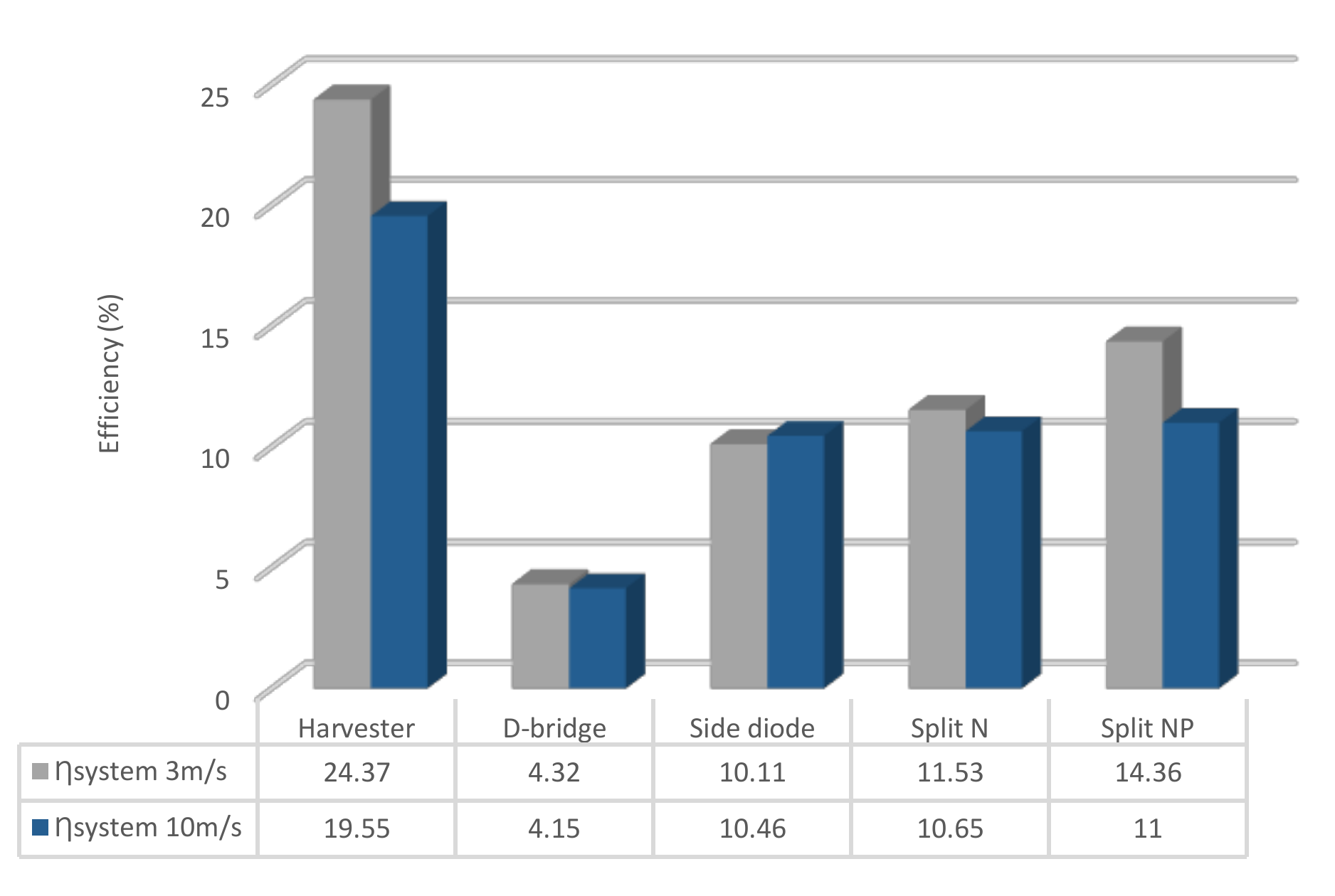
| Harvester | 0.54 | 1.89 | 27 | - | - | 0.54 | 28.24 | 15.25 | 24.37 | 100 | 24.37 |
| D-bridge | 1.05 | 1.79 | 100 | - | - | 0.57 | 5.71 | 3.26 | 12.35 | 35.02 | 4.32 |
| Side diode | 0.4 | 2.4 | 1500 | 0.5 | 200 | 3.08 | 2.05 | 6.32 | 13.6 | 74.32 | 10.11 |
| Split N | 0.85 | 1.57 | 1300 | 0.5 | 333 | 3.20 | 2.46 | 7.88 | 15.37 | 75 | 11.53 |
| Split NP | 0.68 | 2.12 | 1500 | 0.5 | 200 | 3.41 | 2.62 | 8.95 | 17.61 | 81.52 | 14.36 |
| Architec. | Vin (Vpp) | fin (kHz) | Rload (Ω) | D | fsw (kHz) | Vout (V) | Iout (mA) | Pout (mW) | ηgenerator (%) | ηconverter (%) | ηsystem (%) |
|---|---|---|---|---|---|---|---|---|---|---|---|
| Harvester | 2.44 | 8.76 | 27 | - | - | 2.44 | 136.4 | 332.9 | 19.55 | 100 | 19.55 |
| D-bridge | 3.63 | 6.75 | 100 | - | - | 3.1 | 30.6 | 93.7 | 9.72 | 42.64 | 4.15 |
| Side diode | 3.91 | 5.28 | 100 | 0.4 | 500 | 4.19 | 41.95 | 176.0 | 13.01 | 80.04 | 10.46 |
| Split N | 4.09 | 6.42 | 100 | 0.4 | 500 | 4.26 | 42.63 | 181.7 | 13.97 | 76.20 | 10.65 |
| Split NP | 2.31 | 7.77 | 100 | 0.4 | 500 | 4.33 | 43.34 | 187.8 | 14.8 | 74.33 | 11.00 |
| Ref | Topology | Efficiency (%) | Technology | Source |
|---|---|---|---|---|
| [26] | Rectifier + DC/DC (Buck Boost) | 35.64–54.12 | Discrete | Electromagnetic |
| [59] | Rectifier + DC/DC (Frequency up conversion) | 44 | Discrete | Piezoelectric |
| [60] | Rectifier + DC/DC (Buck Boost) | 64.95 | Discrete | Piezoelectric |
| [27] | Rectifier + DC/DC (SECE) | 50–74 | Discrete | Piezoelectric |
| [28] | AC/DC (Boost) | 45 | Discrete | Signal generator |
| This work | AC/DC (Three-phase Split NP) | 74.33–81.52 | Discrete | Electromagnetic |
© 2020 by the authors. Licensee MDPI, Basel, Switzerland. This article is an open access article distributed under the terms and conditions of the Creative Commons Attribution (CC BY) license (http://creativecommons.org/licenses/by/4.0/).
Share and Cite
Pozo, B.; Araujo, J.Á.; Zessin, H.; Mateu, L.; Garate, J.I.; Spies, P. Mini Wind Harvester and a Low Power Three-Phase AC/DC Converter to Power IoT Devices: Analysis, Simulation, Test and Design. Appl. Sci. 2020, 10, 6347. https://doi.org/10.3390/app10186347
Pozo B, Araujo JÁ, Zessin H, Mateu L, Garate JI, Spies P. Mini Wind Harvester and a Low Power Three-Phase AC/DC Converter to Power IoT Devices: Analysis, Simulation, Test and Design. Applied Sciences. 2020; 10(18):6347. https://doi.org/10.3390/app10186347
Chicago/Turabian StylePozo, Borja, José Ángel Araujo, Henrik Zessin, Loreto Mateu, José Ignacio Garate, and Peter Spies. 2020. "Mini Wind Harvester and a Low Power Three-Phase AC/DC Converter to Power IoT Devices: Analysis, Simulation, Test and Design" Applied Sciences 10, no. 18: 6347. https://doi.org/10.3390/app10186347