Modeling Indoor Particulate Matter and Small Ion Concentration Relationship—A Comparison of a Balance Equation Approach and Data Driven Approach


Abstract
:Featured Application
Abstract
1. Introduction
2. Materials and Methods
2.1. Form of the Balance Equation Suitable for Statistical Modelling
2.2. Description of the Statistical Modeling Methodology
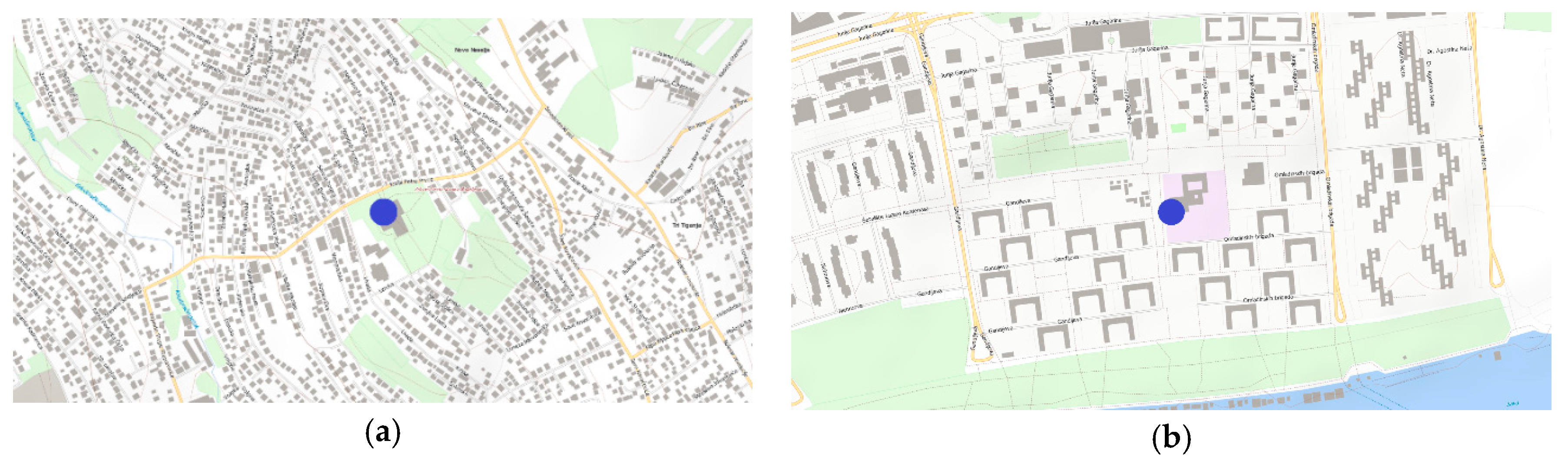
2.3. Description of the Experimental Setup
3. Results
4. Conclusions
- -
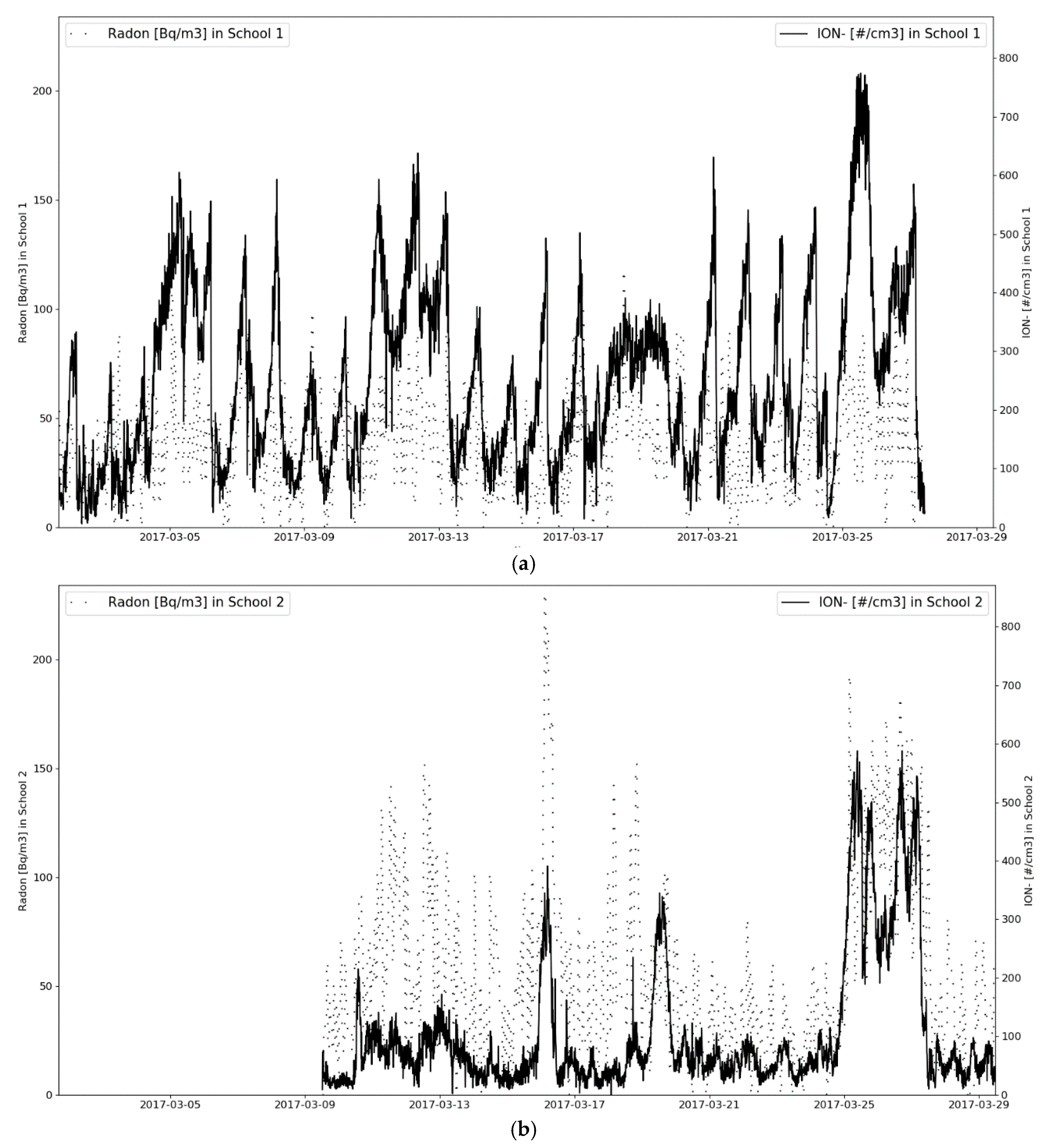
- Descriptive statistics showed that for similar median radon concentrations larger number of nanosized particles corresponds to smaller number of small ions. This observation is coherent with the balance equation.
- -
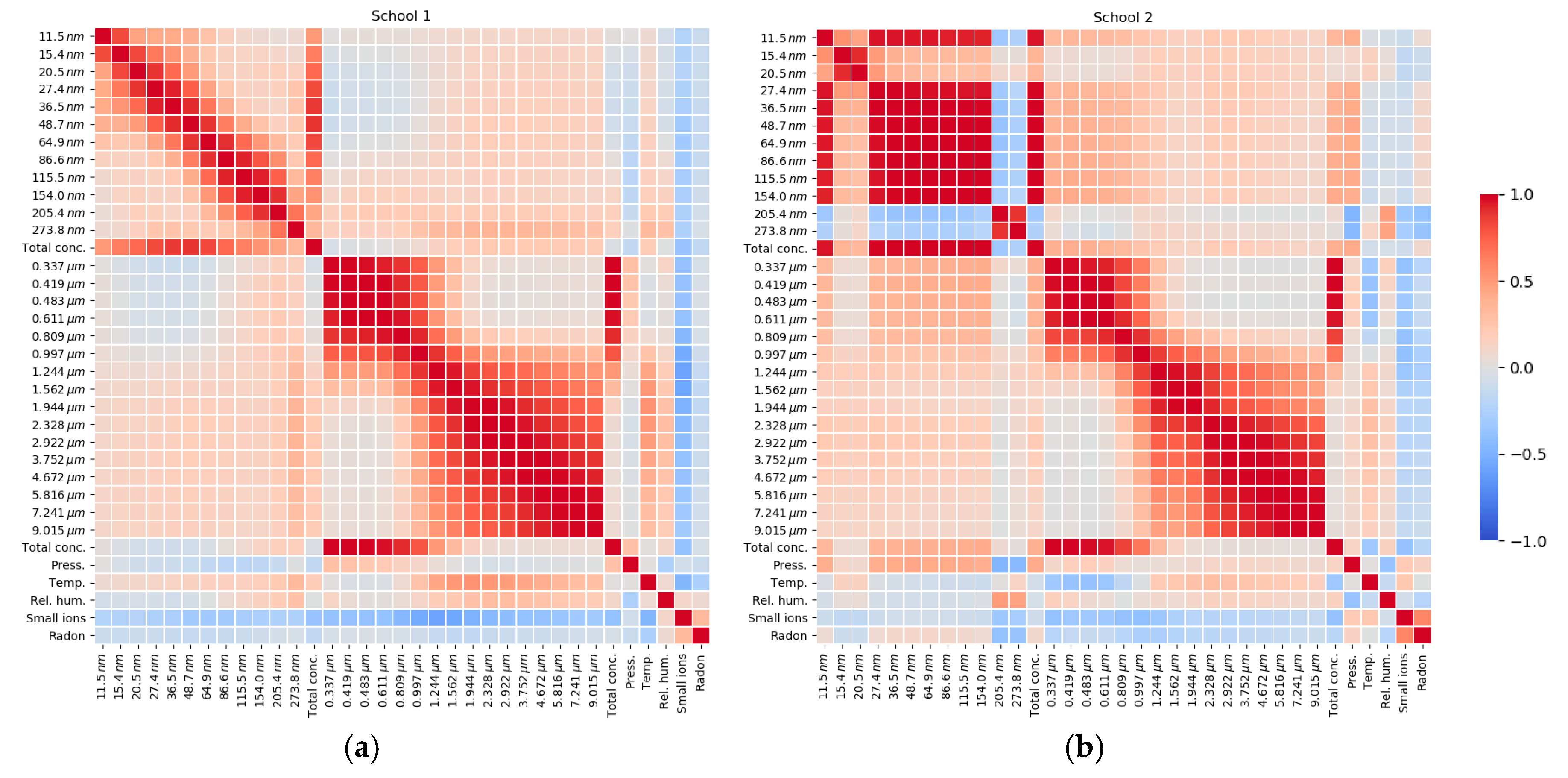
- The linear model derived directly from balance equation allowed estimation of balance equation parameters. The parameters corresponding to the radon term were similar in both schools, indicating similar increase in small ion concentration with radon concentration in both schools. Regarding particulate matter parameters, it was observed that attachment coefficients become larger for particle aggregations corresponding to larger particle diameters, in accordance to theoretical expectations. However, these parameters were different in two schools, possibly due to different air pollution composition.
- -
- The hypothesis that small ion concentration, which may have certain impact on human health and wellbeing, can be predicted based on radon and particulate matter measurements predictors was successfully tested.
- -
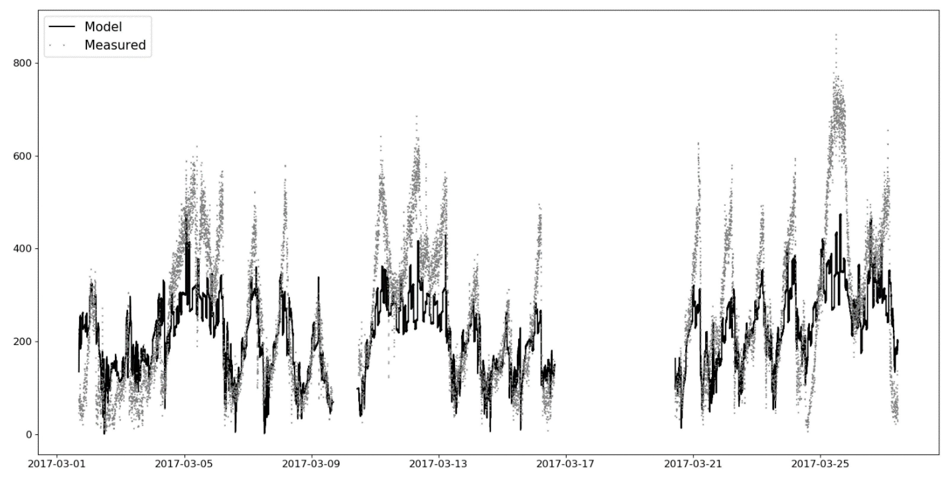
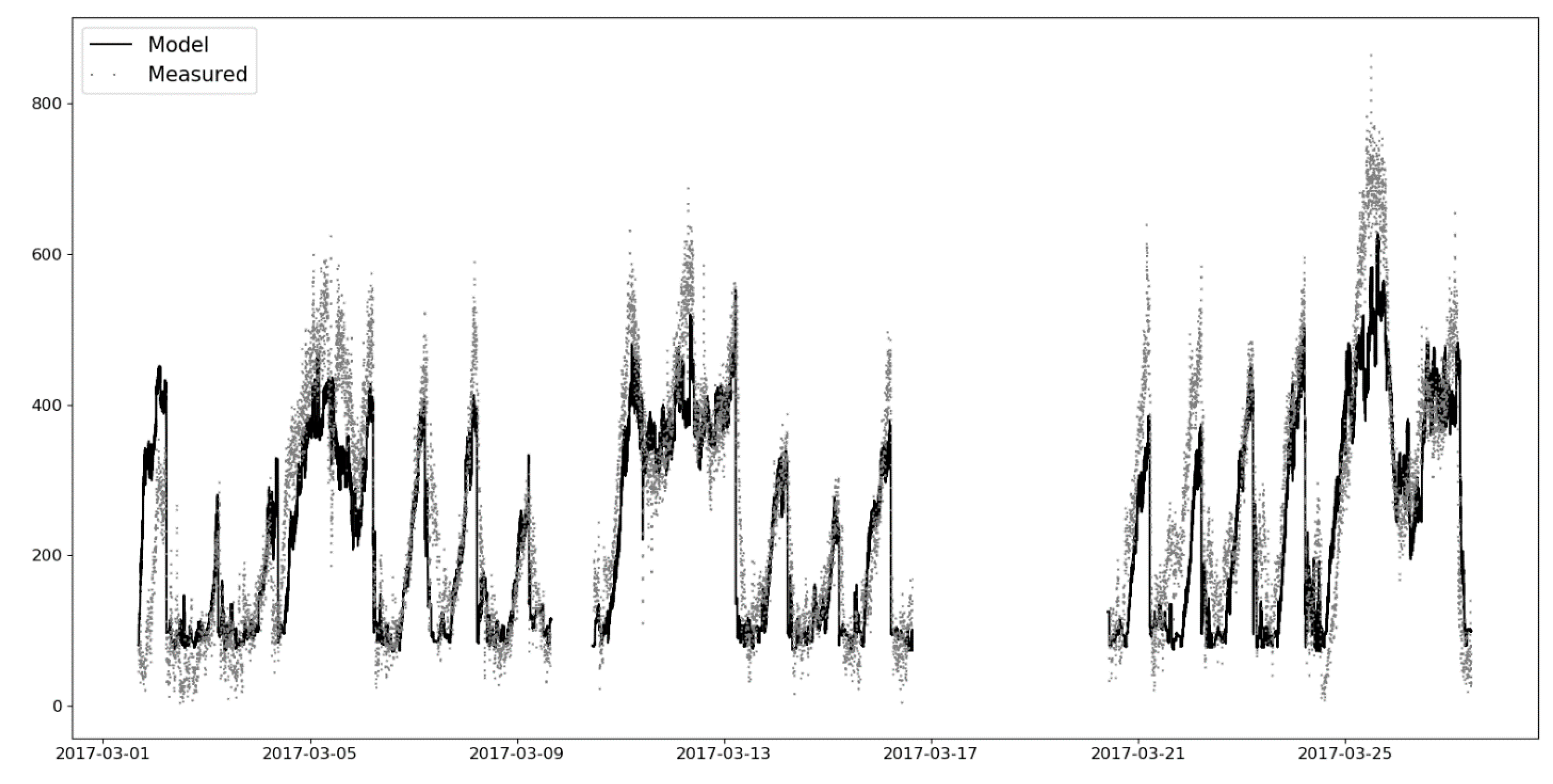
- Explained variance for the linear predictive model was under 0.5, and for the artificial neural network (ANN) predictive model with similar predictors was around 0.7. ANN predictive model has achieved median absolute error of about 40 ions/cm3 on test data.
Author Contributions
Funding
Acknowledgments
Conflicts of Interest
Appendix A
Appendix B

| Instrument | Specification Based on Datasheets, Application Notes and Calibration Certificates | Type of Calibration |
|---|---|---|
| TSI NanoScan SMPS Model 3910 | Relative standard deviations in total concentration 2.7% Sizing of the particles: standard deviations in median particle diameter 1.1% Discrepancy relative to certified size ranges of 20, 60, 80, 200 and 300 nm less than 8%. | NIST traceable using TSI calibration system, conducted in test atmosphere of polystyrene latex particles |
| TSI Optical particle sizer 3330 | Counting efficiency at 0.5 μm (90–110%) Inlet flow: 0.95–1.05 L/min Sizing of 1 μm particles: 90–100% Allowable range is given in parenthesis, calibration certificate includes traceably measured single value. | NIST traceable using TSI calibration system, conducted in test atmosphere of polystyrene latex particles |
| Radon Scout | Sampling type: Diffusion Sensitivity: 1.8 count per minute/kBq/m³ (4 cph/pCi/L) Measurement range: 0…2 MBq/m³ Error: ±5% within the whole range or smaller | Factory calibration, instrument class certified by the US-EPA/NRSB |
| Gerdien-type air ion detector | Sensitivity of the current measurement is limited by AD converter resolution and amounts 1.6 fA. Using Equation (1) in [22], this value equals to 2 ions/cm3. Measuring sensitivity is limited by noise induced by various sources (uncertainties of air-flow, calibration, temperature drift, gain error, etc.) and is experimentally obtained to be ±5 ions/cm3. | Calibrated using Equation (1) in [22] and Keithley 261 small current generator (output signal ~10 fA). Flow tuning was done via hot-wire anemometer. |
Appendix C
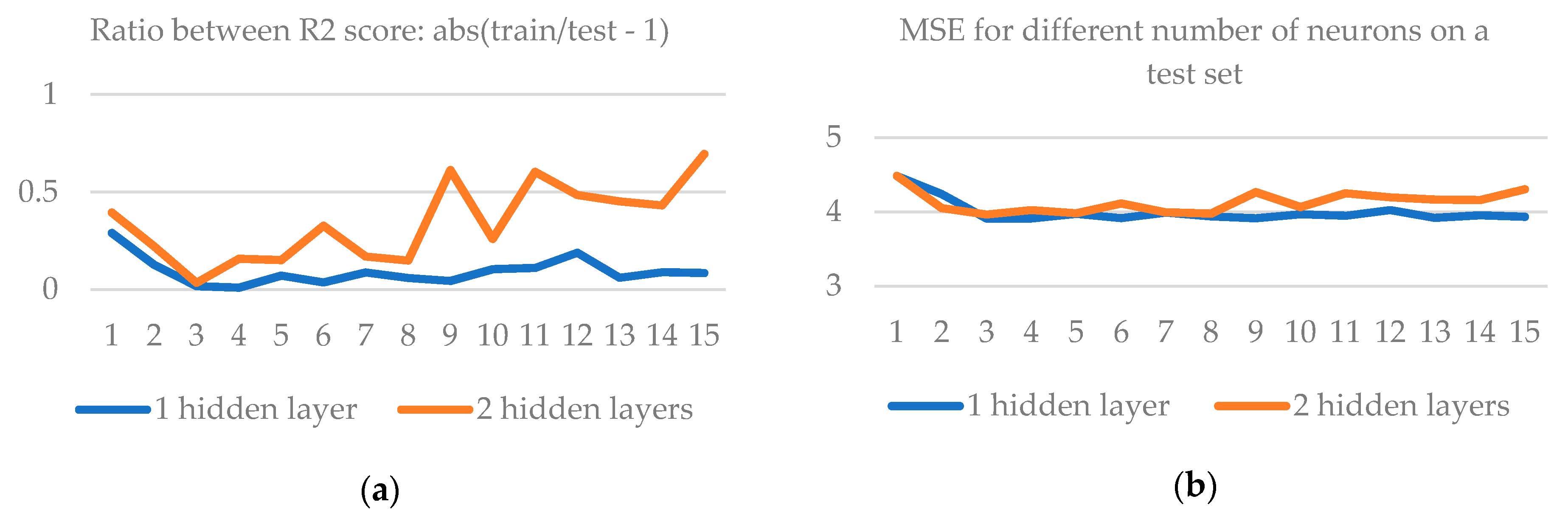
| Hyperparameters | Minimum | Maximum | Step Size |
|---|---|---|---|
| Hidden layers | 1 | 2 | 1 |
| Neurons per hidden layer | 1 | 15 | 1 |
| Neurons in input layers (Radon + PCA components) | 2 | 5 | 1 |
| Early stopping | Not used | ||
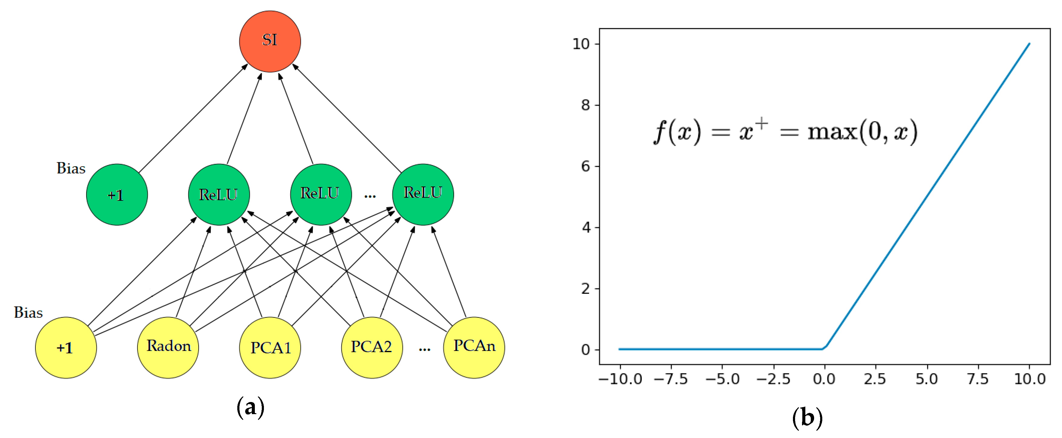
| Activation function | ’relu’ | ||
| Cost function | MSE | ||
| Solver | ‘adam’ | ||


References
- EEA. The European Environment—State and Outlook 2020, Knowledge for Transition to a Sustainable Europe; European Environment Agency: Luxembourg, 2019. [Google Scholar]
- Simoni, M.; Baldacci, S.; Maio, S.; Cerrai, S.; Sarno, G.; Viegi, G. Adverse effects of outdoor pollution in the elderly. J. Thorac. Dis. 2015, 7, 34. [Google Scholar]
- Buka, I.; Koranteng, S.; Osornio-Vargas, A.R. The effects of air pollution on the health of children. Paediatr. Child Health 2006, 11, 513–516. [Google Scholar]
- Höppe, P.; Martinac, I. Indoor climate and air quality. Int. J. Biometeorol. 1998, 42, 1–7. [Google Scholar] [CrossRef] [PubMed]
- Pantelić, G.; Čeliković, I.; Živanović, M.; Vukanac, I.; Nikolić, J.K.; Cinelli, G.; Gruber, V. Qualitative overview of indoor radon surveys in Europe. J. Environ. Radioact. 2019, 204, 163–174. [Google Scholar] [CrossRef] [PubMed]
- EEA. Air Quality in Europe—2018; European Environment Agency: Copenhagen, Denmark, 2018. [Google Scholar]
- Moshammer, H.; Panholzer, J.; Ulbing, L.; Udvarhelyi, E.; Ebenbauer, B.; Peter, S. Acute effects of air pollution and noise from road traffic in a panel of young healthy adults. Int. J. Environ. Res. Public Health 2019, 16, 788. [Google Scholar] [CrossRef] [Green Version]
- WHO. WHO Guidelines for Indoor Air Quality: Selected Pollutants; World Health Organization: Geneva, Switzerland, 2010. [Google Scholar]
- Peters, A.; Wichmann, H.E.; Tuch, T.; Heinrich, J.; Heyder, J. Respiratory effects are associated with the number of ultrafine particles. Am. J. Respir. Crit. Care Med. 1997, 155, 1376–1383. [Google Scholar] [CrossRef]
- Perez, V.; Alexander, D.D.; Bailey, W.H. Air ions and mood outcomes: A review and meta-analysis. BMC Psychiatry 2013, 13, 29. [Google Scholar] [CrossRef] [PubMed] [Green Version]
- Pino, O.; La Ragione, F. There’s something in the air: Empirical evidence for the effects of negative air ions (NAI) on psychophysiological state and performance. Res. Psychol. Behav. Sci. 2013, 1, 48–53. [Google Scholar]
- Jiang, S.-Y.; Ma, A.; Ramachandran, S. Negative air ions and their effects on human health and air quality improvement. Int. J. Mol. Sci. 2018, 19, 2966. [Google Scholar] [CrossRef] [Green Version]
- Health Effects of Exposure to Radon: BEIR VI; National Research Council: Washington, DC, USA, 1999.
- Kim, K.-H.; Kabir, E.; Kabir, S. A review on the human health impact of airborne particulate matter. Environ. Int. 2015, 74, 136–143. [Google Scholar] [CrossRef]
- Rivas, I.; Viana, M.; Moreno, T.; Pandolfi, M.; Amato, F.; Reche, C.; Bouso, L.; Àlvarez-Pedrerol, M.; Alastuey, A.; Sunyer, J. Child exposure to indoor and outdoor air pollutants in schools in Barcelona, Spain. Environ. Int. 2014, 69, 200–212. [Google Scholar] [CrossRef] [PubMed] [Green Version]
- Baloch, R.M.; Maesano, C.N.; Christoffersen, J.; Banerjee, S.; Gabriel, M.; Csobod, É.; Fernandes, E.O.; Annesi-Maesano, I.; Szuppinger, P.; Prokai, R.; et al. Indoor air pollution, physical and comfort parameters related to schoolchildren’s health: Data from the European SINPHONIE study. Sci. Total. Environ. 2020, 739, 139870. [Google Scholar] [CrossRef] [PubMed]
- Schweidler, E. Ueber das Gleichgewicht zwischen ionenerzeugenden und ionenvernichtenden Vorgaengen in der Atmosphaere. S. B. Akad. Wiss. Wien 1918, 128, 947–955. [Google Scholar]
- Donnelly, M.I. A Study of the Nuclear Content of the Atmosphere and the Lifetime of Small Ions in New York City; ETD Collection for Fordham University: New York City, NY, USA, 1950. [Google Scholar]
- Topalović, D.B.; Davidović, M.D.; Jovanović, M.; Bartonova, A.; Ristovski, Z.; Jovašević-Stojanović, M. In search of an optimal in-field calibration method of low-cost gas sensors for ambient air pollutants: Comparison of linear, multilinear and artificial neural network approaches. Atmos. Environ. 2019, 213, 640–658. [Google Scholar] [CrossRef]
- Pedregosa, F.; Varoquaux, G.; Gramfort, A.; Michel, V.; Thirion, B.; Grisel, O.; Blondel, M.; Prettenhofer, P.; Weiss, R.; Dubourg, V. Scikit-learn: Machine learning in Python. J. Mach. Learn. Res. 2011, 12, 2825–2830. [Google Scholar]
- Kingma, D.P.; Ba, J. Adam: A method for stochastic optimization. arXiv 2014, arXiv:1412.6980. [Google Scholar]
- Kolarž, P.; Miljković, B.; Ćurguz, Z. Air-ion counter and mobility spectrometer. Nucl. Instrum. Methods Phys. Res. Sect. B Beam Interact. Materials At. 2012, 219–222. [Google Scholar] [CrossRef]
- Waskom, M.; Botvinnik, O.; O’Kane, D.; Hobson, P.; Ostblom, J.; Lukauskas, S.; Gemperline, D.C.; Augspurger, T.; Halchenko, Y.; Cole, J.B.; et al. mwaskom/seaborn: V0. 9.0 (July 2018). Available online: https://zenodo.org/record/1313201#.X0dZDSMRWUk (accessed on 6 July 2020).
- McKinney, W. Data structures for statistical computing in python. In Proceedings of the 9th Python in Science Conference, Austin, TX, USA, 28 June–3 July 2010; pp. 51–56. [Google Scholar]
- Kuhn, M.; Johnson, K. Applied Predictive Modeling; Springer: Berlin/Heidelberg, Germany, 2013; Volume 26. [Google Scholar]
- University of Arizona, Hydrology & Atmospheric Sciences, Atmospheric Electricity ATMO/ECE 489/589 Spring Term, Lecture Notes. Available online: http://www.atmo.arizona.edu/students/courselinks/spring13/atmo589/ (accessed on 6 July 2020).
- De Vito, S.; Di Francia, G.; Esposito, E.; Ferlito, S.; Formisano, F.; Massera, E. Adaptive machine learning strategies for network calibration of IoT smart air quality monitoring devices. Pattern Recognit. Lett. 2020. [Google Scholar] [CrossRef]
- Iribarne, J.; Cho, H.-R. Atmospheric Physics; D. Reidel Publishing Company: Dordrecht, The Netherlands, 1980. [Google Scholar]
- Jayaratne, E.; Ling, X.; Morawska, L. Observation of ions and particles near busy roads using a neutral cluster and air ion spectrometer (NAIS). Atmos. Environ. 2014, 84, 198–203. [Google Scholar] [CrossRef]


| Negative Small Ions [#/cm3] | Radon [Bq/m3] | Particle conc. 10–420 nm [#/cm3] | Particle conc. 0.3–10 um [#/cm3] | Pressure (atm) | t [°C] | RH [%] | ||||||||
|---|---|---|---|---|---|---|---|---|---|---|---|---|---|---|
| S1 | S2 | S1 | S2 | S1 | S2 | S1 | S2 | S1 | S2 | S1 | S2 | S1 | S2 | |
| Min | 0.0 | 0.0 | 0.0 | 0.0 | 0.0 | 776.5 | 53.2 | 30.4 | 0.97 | 0.98 | 19.60 | 20.12 | 18.97 | 18.87 |
| Max | 871.0 | 643.0 | 118.0 | 234.0 | 95,023.6 | 116,127.2 | 541.9 | 572.6 | 1.00 | 1.01 | 28.81 | 32.62 | 46.14 | 49.18 |
| Mean | 239.9 | 104.8 | 36.8 | 56.5 | 2512.7 | 15,198.2 | 161.1 | 151.1 | 0.98 | 1.00 | 24.24 | 26.64 | 29.77 | 31.20 |
| Med. | 212.0 | 63.0 | 39.0 | 41.0 | 1577.5 | 3724.6 | 142.7 | 132.8 | 0.98 | 1.00 | 24.27 | 26.78 | 29.40 | 30.81 |
| Std. dev | 143.8 | 113.9 | 22.2 | 41.6 | 4283.2 | 31,759.4 | 82.3 | 81.3 | 0.01 | 0.01 | 1.80 | 2.00 | 6.23 | 5.37 |
| (a) | ||||||
| Nanoscan ch. [nm] | 11.5 | 15.4–20.5 | 27.4–64.9 | 86.6–154 | 205–273.8 | |
| S1 | Aggr1 | Aggr2 | ||||
| S2 | Aggr1 | Aggr2 | Aggr3 | |||
| (b) | ||||||
| OPS ch. [μm] | 0.337–0.997 | 1.244–9.015 | ||||
| S1 | Aggr3 | Aggr4 | ||||
| S2 | Aggr4 | Aggr5 | ||||
| Parameters of The Linear Model | Intercept | Radon Term | Aggr1 | Aggr2 | Aggr3 | Aggr4 | |
| School 1 parameters | 291.6 | 1.61 | −5.08 × 10⁻³ | −8.24 × 10⁻³ | −5.08 × 10⁻¹ | −4.88 × 101 | |
| School 1 attachment | 2.87 × 10⁻⁷ | 4.65 × 10⁻⁷ | 2.87 × 10⁻⁵ | 2.75 × 10⁻³ | |||
| Parameters of The Linear Model | Intercept | Radon Term | Aggr1 | Aggr2 | Aggr3 | Aggr4 | Aggr5 |
| School 2 parameters | 111.8 | 1.52 | −2.00 × 10⁻³ | −6.88 × 10⁻³ | −2.08 × 10⁻² | −3.75 × 10⁻¹ | −2.29 × 100 |
| School 2 attachment | 1.05 × 10⁻⁶ | 3.61 × 10⁻⁶ | 1.09 × 10⁻⁵ | 1.97 × 10⁻⁴ | 1.20 × 10⁻³ | ||
© 2020 by the authors. Licensee MDPI, Basel, Switzerland. This article is an open access article distributed under the terms and conditions of the Creative Commons Attribution (CC BY) license (http://creativecommons.org/licenses/by/4.0/).
Share and Cite
Davidović, M.; Davidović, M.; Jovanović, R.; Kolarž, P.; Jovašević-Stojanović, M.; Ristovski, Z. Modeling Indoor Particulate Matter and Small Ion Concentration Relationship—A Comparison of a Balance Equation Approach and Data Driven Approach. Appl. Sci. 2020, 10, 5939. https://doi.org/10.3390/app10175939
Davidović M, Davidović M, Jovanović R, Kolarž P, Jovašević-Stojanović M, Ristovski Z. Modeling Indoor Particulate Matter and Small Ion Concentration Relationship—A Comparison of a Balance Equation Approach and Data Driven Approach. Applied Sciences. 2020; 10(17):5939. https://doi.org/10.3390/app10175939
Chicago/Turabian StyleDavidović, Miloš, Milena Davidović, Rastko Jovanović, Predrag Kolarž, Milena Jovašević-Stojanović, and Zoran Ristovski. 2020. "Modeling Indoor Particulate Matter and Small Ion Concentration Relationship—A Comparison of a Balance Equation Approach and Data Driven Approach" Applied Sciences 10, no. 17: 5939. https://doi.org/10.3390/app10175939