Phonocardiography Signals Compression with Deep Convolutional Autoencoder for Telecare Applications

Abstract

Phonocardiography (PCG) signals that can be recorded using the electronic stethoscopes play an essential role in detecting the heart valve abnormalities and assisting in the diagnosis of heart disease. However, it consumes more bandwidth when transmitting these PCG signals to remote sites for telecare applications. This paper presents a deep convolutional autoencoder to compress the PCG signals. At the encoder side, seven convolutional layers were used to compress the PCG signals, which are collected on the patients in the rural areas, into the feature maps. At the decoder side, the doctors at the remote hospital use the other seven convolutional layers to decompress the feature maps and reconstruct the original PCG signals. To confirm the effectiveness of our method, we used an open accessed dataset on PHYSIONET. The achievable compress ratio (CR) is 32 when the percent root-mean-square difference (PRD) is less than 5%.

1. Introduction

According to the American heart association report, cardiovascular disease (CVD) is the leading global cause of death and it is expected to have more than 22.2 million deaths by 2030 [1]. Auscultation is one of the significant methods for CVD’s monitoring [2]. Besides, heart sound can be used to diagnose heart diseases or to evaluate a human’s physiological condition [3,4]. The electronic stethoscopes exploit the vibrations that are caused by the heartbeats to graphically record the heart sounds called phonocardiography (PCG) signals [5]. The PCG signals provide a non-invasive method for detecting heart valve abnormalities and assisting in diagnosing heart disease. An efficient signal compression method is necessary due to the vast amounts of data that are generated by long-term PCG monitoring. Moreover, telecare, which uses telematics to transmit medical information, has attracted much attention recently, especially for telemedical problems in rural areas [6]. For example, people can put on singlets, which are embedded wearable electrocardiography (ECG) sensors, in order to collect ECG data for telecare purposes [7]. However, for peoples who live in rural areas and have insufficient medical resources, we may use medical electronic stethoscopes to collect the PCG signals and transmit these signals to the doctors at the remote hospital. For the smart healthcare ecosystem, healthcare data privacy and security and data storage issues are some of the most challenging issues and opportunities [8,9]. Most of the current medical tests are done in medical institutions. To check the patients’ health conditions, many of them need to go back and forth between their residences and hospitals. This wastes the patient’s time for medical consultation. Therefore, the development of telecare is a critical issue today. It has created a new way of medical communication, which enables synchronized or asynchronous interaction between physicians and patients, overcoming spatiotemporal barriers, improving medical quality, and increasing convenience. In this work, we focus on the compression of PCG signals by using the deep convolutional autoencoder. Furthermore, we consider the impact of communication link quality [10] and float-point to fixed-point conversion issues. Our proposed method achieves a compression ratio of 32 with the percent root-mean-square difference less than 4.8% under the word-length of 10. Our deep autoencoder can be implemented on the existing lightweight deep learning framework on a smartphone by inspecting the model complexity. The remainder of this paper is organized, as follows. Section 2 briefly describes related work regarding PCG compression problems and background about the deep CNN network. Section 3 details our proposed deep convolutional autoencoder. Section 4 reports the experiments to validate the effectiveness of our work on the PCG compression problems. Section 5 discusses the model complexity issues. Conclusions are drawn in Section 6.

2. Related Work

2.1. Sound Compression

For heart sound compression problems, the conventional performance metrics are compress ratio (CR) and percent root-mean-square difference (PRD) [11]. CR is defined, as follows:

$$\begin{array}{c}\hfill CR=\frac{B_0}{B_1}\end{array}$$

(1)

where $B_0$ and $B_1$ are the data size before and after compression, respectively. PRD can be calculated, as follows:

$$\begin{array}{c}\hfill PRD=\sqrt{\frac{{\sum }_i^N{\left(x_i-{\widehat{x}}_i\right)}^2}{{\sum }_i^N{\left(x_i-{\mu }_x\right)}^2}}\times 100\end{array}$$

(2)

where $x_i$ is the i-th sample in the original signal, and ${\widehat{x}}_i$ denotes the corresponding reconstructed sample. ${\mu }_x$ is the sample mean of the N data samples of the original signals. Note that the mean value of the original signals must be removed to obtain unbiased PRD [12]. Audio compression can be lossless or lossy. It has been shown that lossless compression algorithms rarely obtain a CR larger than 3, while lossy compression algorithms allow attainable CR up to 12 and higher [13]. For example, the value of CR for free lossless audio codec (FLAC) compression is only about 1.94 [14]; and, the value of CR for lossless ECG compression is 2.56 [15]. Additionally, it has been reported that a medical professional felt the necessity of a high CR and can tolerate a PRD as high as 5% [16]. Thus, our design aims to attain a high CR at the values of PRD are less than 5%.

The pioneering work on PCG signals compression has been reported in [17]. The authors proposed using wavelet transform or wavelet packet transform methods in order to compress the original heart sound signals by coefficient thresholding. Their method can further be combined with some lossless compression methods, such as Huffman coding, to increase the compression ratio. The thresholding method based on wavelet energy was reported to reduce the loss caused by compression. At the PRD values of 5.82, the average values of CR are about 40 using the wavelet transform [18]. In [19], the authors proposed using a better wavelet transform method with tunable Q-factor [20]. The optimal value of Q can be found by using the genetic algorithm. In [16], the authors exploited the repetition patterns that were embedded in the PCG signals in order to eliminate their redundancy. After decomposing the PCG signals into the time-frequency domain, the authors proposed clustering the decomposed data to build a dictionary during the training phase. This dictionary is then used to obtain the optimal codebook. They achieved the averaged CR of 17.4 at the averaged PRD 4.87 for PCG signals. For the fetal PCG signals, the authors had reported that the achievable CR was less than 7.5 when the required PRD was less than two by using the compression techniques based on Discrete Cosine Transform (DCT) and Discrete Wavelet Transform (DWT) [21].

2.2. Convolutional Neural Networks

Because audio signals can be stored as one-dimensional (1D) signals, 1D convolutional neural networks (1D CNNs) have been applied to solve many practical problems that traditional signal processing approaches hardly tackle, such as ventricular heartbeats detection [22], speaker recognition [23], speech emotion [24], and environmental sound classification [25]. Other than the audio signals, 1D CNN has been applied to various scenarios, such as human respiration pattern recognition [26], abnormal detection for industrial control systems [27], and contact-less paraparesis detection [28]. In [29], the authors proposed combining the conventional 2D CNN with an autoencoder for the electroencephalogram (EEG) signal compression problems. The autoencoder aims to reconstruct its input based on the neural network in an unsupervised learning manner [30].

Let $\mathbf{x}$ be the input to convolution layer of length N and $\mathbf{h}$ be the kernel of size K. Let $\mathbf{y}$ be the output of the non-causal 1D convolution between $\mathbf{x}$ and $\mathbf{h}$. We can express the n-th element of $\mathbf{y}$ as follows [31]:

$$\begin{array}{c}\hfill y\left(n\right)=\sum _{k=0}^{K}x\left(n+k+(s-1)\right)h\left(k\right)\end{array}$$

(3)

where $x\left(n\right)$ and $h\left(n\right)$ represent the n-th element of $\mathbf{x}$ and $\mathbf{h}$, respectively; s denotes the stride for shifting the kernel window. Note that the length of output vector $\mathbf{y}$ is not equal to the length of output vector $\mathbf{x}$, and this can be avoided by zero-padding operation for the input vector. In each CNN layer, 1D forward propagation can be expressed, as follows:

$$\begin{array}{c}\hfill x_k^{\ell }=\sum _{i=1}^{N_{\ell -1}}conv1D\left(w_{ik}^{\ell -1},s_i^{\ell -1}\right)+b_k^{\ell }\end{array}$$

(4)

where $x_k^{\ell }$ denotes the input of the k-th neuron at the ℓ-th layer of the CNN; $b_k^{\ell }$ represents the corresponding bias; $s_i^{\ell -1}$ is the output of the i-th neuron at the $(\ell -1)$-th layer; $w_{ik}^{\ell -1}$ is the kernel from the i-th neuron at the $(\ell -1)$-th layer to the k-th neuron at the ℓ-th layer; $conv1D\left(·,·\right)$ is used to perform 1D convolution operation, as described in (3). The output of the k-th neuron at the ℓ-th layer $y_k^{\ell }$ can be expressed, as follows:

$$\begin{array}{c}\hfill y_k^{\ell }=f\left(x_k^{\ell }\right)\end{array}$$

(5)

where $f\left(·\right)$ is the non-linear activation function. Possible activation functions could be sigmoid function, hyperbolic tangent, and rectified linear unit (ReLU). Note that $y_k^{\ell }$ may be further processed by pooling operation to create downsampled or pooled feature maps, a summarized version of the features detected in the input. Two standard functions used in the pooling operation are average pooling and maximum pooling (MaxPool). The average and MaxPool operations calculate the average and maximum values for each patch on the feature map. For example, the MaxPool with a factor of P can be expressed, as follows:

$$\begin{array}{c}\hfill s_k^{\ell }\left(n\right)=Max\left\{y_k^{\ell }\left(n\right),y_k^{\ell }(n-1),\dots ,y_k^{\ell }(n-P+1)\right\}.\end{array}$$

(6)

2.3. Autoencoder

Autoencoders have been widely used in data denoising [32,33,34] and data compression [35] applications. An autoencoder comprises encoder and decoder parts. The encoder translates an input vector $\mathbf{x}$ with length N to a hidden representation $\mathbf{y}$ with length M. The transform can be expressed, as follows:

$$\begin{array}{c}\hfill \mathbf{y}=f\left(\mathbf{W}·\mathbf{x}+\mathbf{b}\right),\end{array}$$

(7)

where $\mathbf{W}$ denotes the weight matrix of size $M\times N$, $\mathbf{b}$ represents the bias vector of size $M\times 1$, and $f\left(·\right)$ denotes the transformation function, which is non-linear in general. Note that for data compression purposes, $N\gg M$ holds. On the other hand, the decoder translates the hidden representation $\mathbf{y}$ to a reconstructed representation $\widehat{\mathbf{x}}$ with the same length of $\mathbf{x}$. The demapping process can be expressed, as follows:

$$\begin{array}{c}\hfill \widehat{\mathbf{x}}=g\left({\mathbf{W}}^{\prime }·\mathbf{y}+{\mathbf{b}}^{\prime }\right),\end{array}$$

(8)

where ${\mathbf{W}}^{\prime }$ denotes the weight matrix of size $N\times M$, ${\mathbf{b}}^{\prime }$ represents the bias vector of size $N\times 1$, and $g\left(·\right)$ denotes the demapping function, which is non-linear in general. The parameters associated with the autoencoder are adjusted by minimizing the following cost function J:

$$\begin{array}{c}\hfill J\left(\mathbf{W},\mathbf{b},{\mathbf{W}}^{\prime },{\mathbf{b}}^{\prime }\right)=\frac{1}{L}\sum _{\ell =1}^L\left|\right|{\mathbf{x}}_{\ell }-{\widehat{\mathbf{x}}}_{\ell }{\left|\right|}^2,\end{array}$$

(9)

where L denotes the length of the training dataset.

3. Method

3.1. Data Pre-Processing

Before applying the measured data into the proposed deep convolutional autoencoder model, the data is pre-processed as follows:

• Normalization: the data are normalized, such that the values of all data sets are mapped into the ranges of [0, 1].
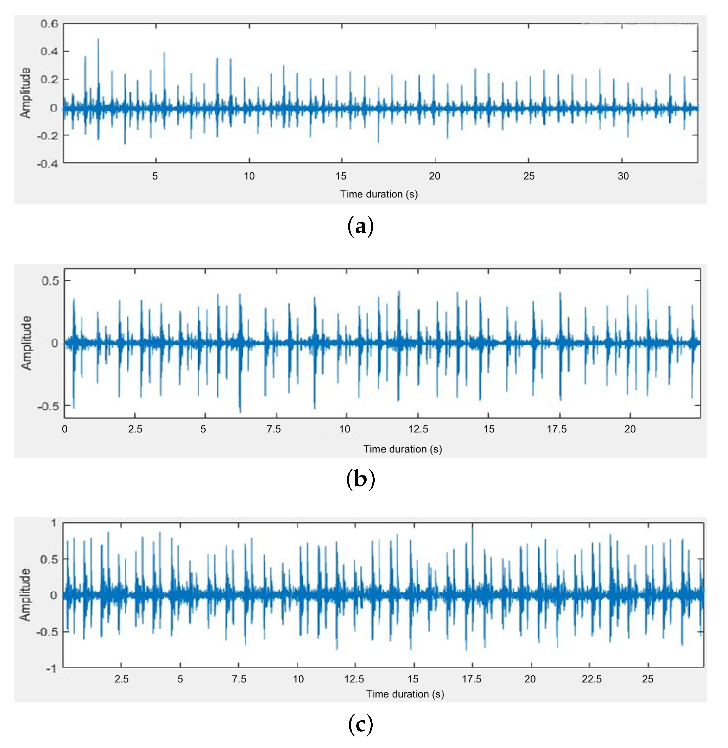
• Segmentation: we edit the heart sound into several fixed-length segments. The time duration of each segment is 3 s, which corresponds to 6000 samples at the sampling rate of 2 kHz. Note that each segment contains roughly four or five cardiac cycles.
• Overlapping: we apply a sliding window on the data segmentation to implement the data augmentation. Except for the first segment, each segment is overlapped with its previous segment by 93.33%, i.e., each segment has 400 new samples and keeps 5600 existing samples in the previous segment. It has been reported that such a time-shift-based data augmentation method is useful to prevent overfitting [36] when training the CNN networks [37].

3.2. Feature Selection

It has been reported that the hidden semi-Markov model (HSMM) heart sound segmentation method could correctly decompose a cardiac cycle into four parts: S1, systole, S2, and diastole periods [38]. We propose using S1 and S2 signals as the features to train the deep convolutional autoencoder. Thus, for each segment, we null all samples that correspond to the systole and diastole periods and keep other samples in a segment.

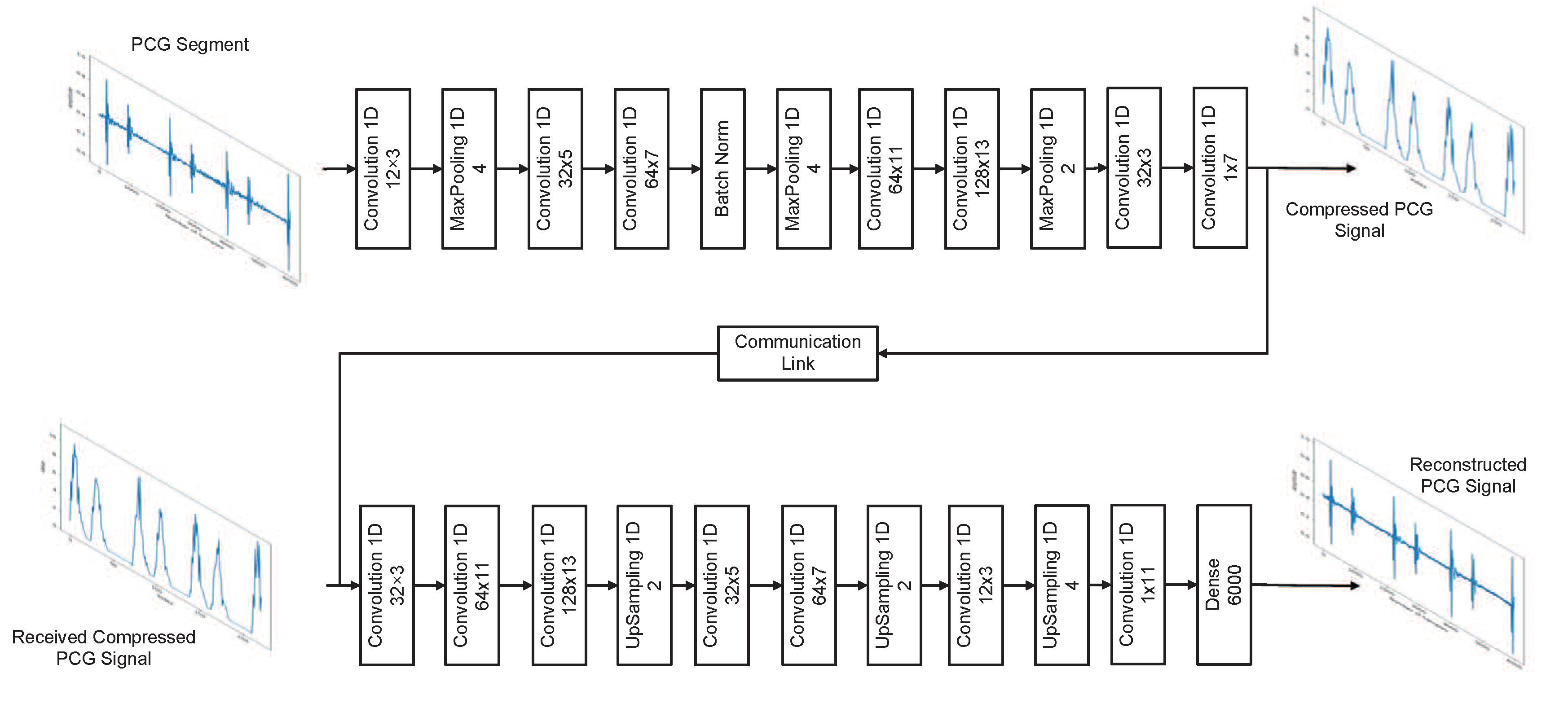
3.3. Proposed Network Model for the Deep Convolutional Autoencoder

Figure 1 depicts the system model in this work. With the aid of medical professionals, such as nurses, the patients who live in rural areas can regularly collect their PCG signals using electronic stethoscopes; then, an encoder continuously compresses the PCG signals before transmitting these compressed data to the remote site via a noisy communication link. Doctors use a decoder to continuously decompress the received compressed PCG signals at the remote site, so that doctors can virtually auscultate the patients’ heart sounds without meeting with patients. Inspired by the pioneering works about the design of the deep neural network [39,40], we combine one to two convolutional networks with one max-pooling layer as a basic unit to build our proposed network architecture at the encoder side; on the decoder side, we combine one to two convolutional networks with one upsampling layer as a basic unit. Empirically, we keep stacking the basic units until overfitting happened in order to determine the depth of our network model. The details about the encoder and decoder are listed

Table 1. Detail parameters for each layer in the proposed encoder.

No.	Layer Function	No. of Filter × Kernel Size	Activation Function	No. of Trainable Param.	Output Size
1	Conv 1D	12 × 3	ReLU	48	6000 × 12
2	MaxPool 1D	-	-	0	1500 × 12
3	Conv 1D	32 × 5	ReLU	1952	1500 × 32
4	Conv 1D	64 × 7	ReLU	14,400	1500 × 64
5	Batch Norm	-	-	256	1500 × 64
6	MaxPool 1D	-	-	0	375 × 64
7	Conv 1D	64 × 11	ReLU	45,120	375 × 64
8	Conv 1D	128 × 13	ReLU	106,624	375 × 128
9	MaxPool 1D	-	-	0	187 × 128
10	Conv 1D	32 × 3	ReLU	12,320	187 × 32
11	Conv 1D	1 × 7	ReLU	225	187 × 1

and

Table 2. Detail parameters for each layer in the proposed decoder.

No.	Layer Function	No. of Filter × Kernel Size	Activation Function	No. of Trainable Param.	Output Size
1	Conv 1D	32 × 3	ReLU	128	187 × 32
2	Conv 1D	64 × 11	ReLU	22,592	187 × 64
3	Conv 1D	128 × 13	ReLU	106,624	187 × 128
4	Upsampling	-	-	0	374 × 128
5	Conv 1D	32 × 5	ReLU	20,512	374 × 32
6	Conv 1D	64 × 7	ReLU	14,400	374 × 64
7	Upsampling	-	-	0	748 × 64
8	Conv 1D	12 × 3	ReLU	2316	748 × 12
9	Upsampling	-	-	0	2992 × 12
10	Conv 1D	1 × 11	ReLU	133	2992 × 1
11	Dense	6000	Sigmoid	17,958,000	6000

, respectively.

For the encoder, we fed one segment, which contains 6000 samples, into the first layer. After this convolutional operation with 12 1D filters, each with a kernel size of three and zero paddings, its output size is 6000 × 12. We can treat that 12 features are extracted from one segment by the first convolutional network. Subsequently, the one-dimensional max-pooling operation reduces the signal length by four, i.e., the output of the MaxPool 1D layer is 1500 × 12. After the consecutive convolution and max pooling operations, the final layer outputs a vector with length 187. This means the encoder compresses each segment with 6000 samples into each feature map with 187 samples. Note that one batch normalization (Batch Norm) was used in the encoder, such that a stable distribution of activation values throughout training to alleviate the internal covariate shift problems [41].

Table 2 lists the decoder’s detailed architecture, which decompresses each feature map with 187 samples to reconstruct the corresponding PCG segments, each with 6000 samples. Note that, except for the convolutional network and up-sampling operations, the last layer is a fully connected network (Dense) reconstruct the original segment. The total number of trainable parameters for the encoder and decoder are 180,945 and 18,124,705, respectively. This implies the computational cost at the encoder is much less than that at the decoder. Note that the PCG signals can continuously partition into segments and then be compressed with the proposed encoders. The remote side then continuously receives each compressed feature maps. After decoding, the decompressed segments can be used to combine into the original PCG signals. Thus, even though each segment contains roughly only four or five cardiac cycles, which may be insufficient for diagnostic or monitoring purposes, our segment-by-segment signal processing approach could achieve a good CR and a low PRD without compromising continuity for the long-term monitoring.

4. Experiments

4.1. Dataset

We used an open accessed dataset, which comprises nine heart sound databases that were collected by various organizations, provided by PHYSIONET [42]. Due to a large number of tested subjects and long recording time, we choose the database that was collected by the Dalian University of Technology heart sounds database (DLUTHSDB) from these nine sound databases as our experimental dataset. In this dataset, subjects included 174 healthy volunteers and 335 patients with coronary artery disease. PHYSIONET resamples the original waveform at 2 kHz. Figure 2 illustrates three recorded heart sound in the DLUTHSDB database.

4.2. Results

The experiments were conducted on the Tensorflow framework. First, we evaluate the impact of segment length on the resulting PRD and the computational complexity and determine the suitable segment length to our proposed model. Next, we try to increase the CR with a tolerable PRD. Third, we consider fixed-point and communication link quality issues for practical implementation.

4.2.1. Segment Length Evaluation

During the training phase, the batch size is chosen as 60, and the number of the epoch is set to 200. Meanwhile, we use conventional adaptive moments (Adam) optimizer [43] in order to obtain better results. The main parameters associated with the Adam optimizer are learning rate = 0.01, hyper-parameters ${\beta }_1=0.9$ and ${\beta }_2=0.999$, weight decay factor $\lambda$ = ${10}^{-5}$. Because each audio file’s length in the data set is not the same, we first divided them into segments and then randomly split into approximately 80% for training, 10% for validation, and 10% for testing, respectively.

We fix the CR as 27 and evaluate the resulting PRD under various segment lengths (see Figure 3). Note that the segment length of 2000 or 3000 samples contains roughly two or three cardiac cycles; the segment length of 6000 samples contains roughly four or five cardiac cycles, and the segment length of 8000 samples contains roughly six or seven cardiac cycles. The evaluation results are listed in

Table 3. Segment Length Evaluation at CR = 27.

Segment Length	2000	3000	6000	8000
Total Segments	220,470	146,980	73,490	55,117
PRD	4.696%	4.668%	4.495%	4.571%
Parameters	≈4.3 × 10${}^6$	≈9.3 × 10${}^6$	≈3.6 × 10${}^7$	≈6.4 × 10${}^7$

, in which we can observe that the longer segment length leads to higher computational cost, and the segment length of 6000 achieves the lowest PRD. Thus, we choose the samples in a segment as 6000.

As shown in Figure 4, we observe that for the time duration of 3 s (segment length of 6000), the details contained in the compressed signals are less than that for the time duration of 4 s (segment length of 8000) (see Figure 4a,c). However, the comparisons between original data with the reconstructed signal reveal that the time duration of 3 s (segment length of 6000) has a less PRD (see Figure 4b,d–f). Thus, we inferred that too many details in a compressed signal might not lead to a better PRD performance. This could explain why a network model with a more significant number of trainable parameters fails to result in better training results.

4.2.2. Compression Ratio Evaluation

It has been shown that higher values of CR result in larger values of PRD. Given that PRD’s desired values are less than 5%, we would like to evaluate the attainable best CR in this Section.

During the training phase, the batch size is chosen as 60, and the number of the epoch is set to 400. We fix the length of the segment of 6000, and the total number of segments is about $7.2\times {10}^3$. The dataset was randomly split into approximately 80% for training, 10% for validation, and 10% for testing. Meanwhile, we use the conventional Adam optimizer, as we have described in Section 4.2.1. The evaluation results are shown in

Table 4. CR Evaluation at a segment length of 6000.

CR	27	30	32	36
Length for each Compressed Segment	222	200	187	166
Epoch	389	368	362	345
PRD	4.416%	4.540%	4.601%	4.972%

. Although the PRD corresponding to CR = 36 is less than the target PRD (5%), if we further considered the fixed-point computation issue, the resulting PRD may not meet the target PRD. Thus, we choose the value of CR as 32 in the rest of this paper.

4.2.3. Fixed-Point Issues

We consider the fixed-point operation issues for the proposed network architecture to reduce the computational cost of the floating-point operation.

Table 5. The range of weight and bias for the proposed network model.

	Max. Weight	Min. Weight	Max. Bias	Min. Bias
Encoder
Layer 1	0.39540452	−0.9235797	0.01453111	−0.023743011
Layer 2	-	-	-	-
Layer 3	0.6052952	−0.8330374	0.033396643	−0.054285403
Layer 4	0.48703766	−0.7313971	0.1558624	−0.09510201
Layer 5	0.3240463	0.9359407	0.054475907	−0.06052749
Layer 6	-	-	-	-
Layer 7	0.24897571	−0.49508682	0.052439176	−0.082461566
Layer 8	0.24272417	−0.68896836	0.10369389	−0.098621696
Layer 9	-	-	-	-
Layer 10	0.39203942	−0.47291782	0.10768643	−0.08815236
Layer 11	0.52950436	−0.3272031	0.13014604	0.13014604
Decoder
Layer 1	0.31976736	−0.33887985	0.17345946	−0.12427106
Layer 2	0.33624372	−0.7039436	0.11306709	−0.10122227
Layer 3	0.38897622	−0.6367118	0.04357844	−0.16350096
Layer 4	-	-	-	-
Layer 5	0.7269572	−0.2668362	0.02763602	−0.04904448
Layer 6	0.5182032	−0.63450485	0.039916832	−0.038330693
Layer 7	-	-	-	-
Layer 8	0.5744175	−0.563132	0.024111861	−0.024702776
Layer 9	-	-	-	-
Layer 10	0.25195208	−0.30334103	0.01607588	0.01607588
Layer 11	0.44964585	−0.87970144	0.071185686	0.071185686

lists the maximum and minimum values of both weights and biases for each layer at the encoder and the decoder sides. Note that layers 2, 6, and 9 are max-pooling layers at the encoder side; the layers 4, 7, and 9 are up-sampling layers at the decoder side.

Table 6. Word-length evaluation.

Word-Length	Fractional Length	PRD(%)
Floating-32	-	4.6015
Fixed-20	17	4.6031
Fixed-16	13	4.6127
Fixed-12	9	4.6437
Fixed-11	8	4.6639
Fixed-10	7	4.7923
Fixed-9	6	5.2162
Fixed-8	5	6.1334

shows the evaluation results in fixed-point cases. Thus, we choose the word length as 10 in the rest of this paper. Note that we assign one bit for the sign bit, two bits for integer parts, and the remaining seven bits for fractional parts.

4.3. Communication Link Quality Issues

Besides the segment length, CR, and the fixed-point factors, we further consider the impact of communication link quality on the resulting PRD. We simply model the link quality using the artificially induced bit error rate (BER) from the communication link and compare our proposed method with the conventional DCT method. The evaluation results can be found in

Table 7. Evaluation of the impact of communication link quality on the root-mean-square difference (PRD) and the quality score (QS).

BER	DCT Method @ CR of 15		Proposed Method @ CR of 32
	PRD	QS	PRD	QS
${10}^{-2}$	43.700%	0.343	7.435%	4.304
${10}^{-3}$	14.048%	1.068	5.094%	6.282
${10}^{-4}$	6.436%	2.331	4.815%	6.646
${10}^{-5}$	5.536%	2.710	4.793%	6.676
${10}^{-6}$	5.491%	2.732	4.793%	6.676
0	5.480%	2.737	4.792%	6.678

. To have a fair comparison, we set the CR as 15 for the DCT method, so that the resulting PRD is close to 5% in the simulation. As shown in the last row in Table 7, when there is no transmission error, i.e., BER = 0, the DCT method could achieve PRD of 5.48% at CR of 15 while our method could attain PRD of 4.792% at CR of 32. We can observe that the resulting PRD with the DCT compression method exhibits a significant drop when the value of BER is higher than ${10}^{-3}$; however, our proposed method shows the smooth performance when the communication link quality becomes noisier. Similar results could also be observed from the QS index. This could imply that we method has a better immunity against transmission errors. Note that the CR for the DCT and our methods are different in Table 7. Thus, we further consider a performance metric “quality score” (QS), which is the ratio between the CR and the PRD, i.e., QS = CR/PRD. The QS index is useful when the values of CR for different compression methods are different [44]. When ignoring communication errors, our method could reach a little lower PRD and a significantly higher CR than the DCT-based compression method. That is, our proposed method exhibits a higher QS than the conventional DCT method could achieve. However, the computational cost of the DCT method is less than our method.

5. Discussion

For the telecare application, it is desired that the hardware cost or computational complexity of the proposed method is affordable to people in rural areas. We use the number of multiply-accumulate (MAC) operations as the performance metric to evaluate the model complexity. In our proposed model, the computation-intensive operation is mainly on the convolutional layer and the fully-connected layer. For a convolutional layer with the kernel size of K, the number of the filter of $C_{out}$, input length of $W_{out}$, and the number of input layer $C_{in}$, the resulting number of MAC at the encoder and decoder side are listed in

Table 8. The number of multiply-accumulate (MAC) of the convolutional layers at the encoder side.

Layer ID	$({\mathit{W}}_{\mathit{out}},{\mathit{C}}_{\mathit{in}},{\mathit{C}}_{\mathit{out}},\mathit{K})$	Required Number of MAC
Conv 1D (12, 3)	(6000, 1, 12, 3)	216,000
Conv 1D (32, 5)	(1500, 12, 32, 5)	2,880,000
Conv 1D (64, 7)	(1500, 32, 64, 7)	21,504,000
Conv 1D (64, 11)	(375, 64, 64, 11)	16,896,000
Conv 1D (128, 13)	(375, 64, 128, 13)	39,936,000
Conv 1D (32, 3)	(187, 128, 32, 3)	22,978,576
Conv 1D (1, 7)	(187, 32, 1, 7)	41,888

and

Table 9. The number of MAC of the deep convolutional layers at the decoder side.

Layer ID	$({\mathit{W}}_{\mathit{out}},{\mathit{C}}_{\mathit{in}},{\mathit{C}}_{\mathit{out}},\mathit{K})$	Required Number of MAC
Conv 1D (32, 3)	(187, 1, 32, 3)	17,952
Conv 1D (64, 11)	(187, 32, 64, 11)	4,212,736
Conv 1D (128, 13)	(187, 64, 128, 13)	19,914,752
Conv 1D (32, 5)	(374, 128, 32, 5)	7,659,520
Conv 1D (64, 7)	(374, 32, 64, 7)	5,361,664
Conv 1D (12, 3)	(748, 64, 12, 3)	1,723,392
Conv 1D (1, 11)	(2,992, 12, 1, 11)	394,944

, respectively. Moreover, the full connection layer at the decoder side has 2992 inputs and 6000 outputs, i.e., the number of MACs is 17,952,000. In summary, the number of GMAC is around 0.08 and 0.06 at the encoder and decoder sides, respectively. Besides, we use a tool called “SCALE-Sim” in order to evaluate the required cycles performed on the “Eyeriss” chips [45]. For the encoder, the seven “Conv 1D” layers listed in Table 8 require 6016, 22,960, 145,386, 118,491, 279,700, 21,088, and 3906 cycles on the Eyeriss chips, respectively. The total number of cycles is about $5.98\times {10}^5$ cycles. The ratio of the required number of cycles at the encoder of our method to the MobileUNet, which runs MobileNet [46,47] on U-Net [48], is about one third (see

Table 10. Expected cycles on Eyeriss chips. (a) MobileUNet and (b) proposed architecture.

(a) MobileUNet		(b) Proposed Architecture
Layer	Eyeriss (Cycle)	Layer	Eyeriss (Cycle)
Layer1	111,969	Layer1	6016
Layer2	291,000	Layer2	22,960
Layer3	188,672	Layer3	145,386
Layer4	148,416	Layer4	118,491
Layer5	190,208	Layer5	279,700
Layer6	282,336	Layer6	21,088
Layer7	348,928	Layer7	3906
Layer8	73,728
Layer9	171,536
Layer10	134,592
Total	1,941,385	Total	597,547

). It has been shown that MobileUNet implements real-time deep learning in mobile applications [49]. Thus, the model complexity of our proposed model is affordable for a consumer-grade smartphone.

6. Conclusions

In this paper, we have proposed a convolutional autoencoder’s architecture for the compression of 1D PCG signals. When the input segment length of 6000 samples, the achievable CR is 32 under the constraint that the corresponding PRD is less than 5%. The proposed method is more robust than the DCT compression method when considered the impact of the link quality. As the BER rose from ${10}^{-4}$ to ${10}^{-3}$, the DCT method increased the PRD by about 7.6%, whereas our proposed method increased the PRD by only about 0.3%. We also considered the fix-point issue. When comparing the case of floating-point representation, we observed that the evaluation results have shown that the resulting PRD was slightly increased by 0.2% as the word-length of 10 bits with Q3.7 format. Our future work is jointly considered the denoising and data compression tasks for the PCG signals while using the deep convolutional autoencoder.

References

1. Virani, S.S.; Alonso, A.; Benjamin, E.J.; Bittencourt, M.S.; Callaway, C.W.; Carson, A.P.; Chamberlain, A.M.; Chang, A.R.; Cheng, S.; Delling, F.N.; et al. Heart Disease and Stroke Statistics—2020 Update: A Report from the American Heart Association. Circulation 2020, 141, e139–e596. [Google Scholar] [CrossRef] [PubMed]
2. Martins, M.; Gomes, P.; Oliveira, C.; Coimbra, M.; da Silva, H.P. Design and Evaluation of a Diaphragm for Electrocardiography in Electronic Stethoscopes. IEEE Trans. Biomed. Eng. 2020, 67, 391–398. [Google Scholar] [CrossRef] [PubMed]
3. Babu, K.A.; Ramkumar, B.; Manikandan, M.S. Automatic Identification of S1 and S2 Heart Sounds Using Simultaneous PCG and PPG Recordings. IEEE Sensors J. 2018, 18, 9430–9440. [Google Scholar] [CrossRef]
4. Abdel-Alim, O.; Hamdy, N.; El-Hanjouri, M.A. Heart Diseases Diagnosis Using Heart Sounds. In Proceedings of the Nineteenth National Radio Science Conference, Alexandra, Egypt, 19–21 March 2002; pp. 634–640. [Google Scholar] [CrossRef]
5. Sumarna; Astono, J.; Purwanto, A.; Agustika, D.K. The Improvement of Phonocardiograph Signal (PCG) Representation Through the Electronic Stethoscope. In Proceedings of the 2017 4th International Conference on Electrical Engineering, Computer Science and Informatics (EECSI), Yogyakarta, Indonesia, 19–21 September 2017; pp. 1–5. [Google Scholar] [CrossRef]
6. Habibzadeh, H.; Dinesh, K.; Rajabi Shishvan, O.; Boggio-Dandry, A.; Sharma, G.; Soyata, T. A Survey of Healthcare Internet of Things (HIoT): A Clinical Perspective. IEEE Internet Things J. 2020, 7, 53–71. [Google Scholar] [CrossRef]
7. Ozkan, H.; Ozhan, O.; Karadana, Y.; Gulcu, M.; Macit, S.; Husain, F. A Portable Wearable Tele-ECG Monitoring System. IEEE Trans. Instrum. Meas. 2020, 69, 173–182. [Google Scholar] [CrossRef]
8. Aazam, M.; Zeadally, S.; Harras, K.A. Health Fog for Smart Healthcare. IEEE Consum. Electron. Mag. 2020, 9, 96–102. [Google Scholar] [CrossRef]
9. Qadri, Y.A.; Nauman, A.; Zikria, Y.B.; Vasilakos, A.V.; Kim, S.W. The Future of Healthcare Internet of Things: A Survey of Emerging Technologies. IEEE Commun. Surv. Tuts. 2020, 22, 1121–1167. [Google Scholar] [CrossRef]
10. Fang, S.; Yang, Y. The Impact of Weather Condition on Radio-Based Distance Estimation: A Case Study in GSM Networks with Mobile Measurements. IEEE Tran. Veh. Technol. 2016, 65, 6444–6453. [Google Scholar] [CrossRef]
11. Kim, S.; Hwang, D. Murmur-adaptive compression technique for phonocardiogram signals. Elect. Lett. 2016, 52, 183–184. [Google Scholar] [CrossRef]
12. Blanco-Velasco, M.; Cruz-Roldán, F.; Godino-Llorente, J.; Blanco-Velasco, J.; Armiens-Aparicio, C.; López-Ferreras, F. On the use of PRD and CR parameters for ECG compression. Med. Eng. Phys. 2005, 27, 798–802. [Google Scholar] [CrossRef]
13. Hans, M.; Schafer, R.W. Lossless compression of digital audio. IEEE Signal Process. Mag. 2001, 18, 21–32. [Google Scholar] [CrossRef] [Green Version]
14. Huang, H.; Shu, H.; Yu, R. Lossless audio compression in the new IEEE Standard for Advanced Audio Coding. In Proceedings of the 2014 IEEE International Conference on Acoustics, Speech and Signal Processing (ICASSP), Florence, Italy, 4–9 May 2014; pp. 6934–6938. [Google Scholar] [CrossRef]
15. Chen, S.; Luo, G.; Lin, T. Efficient fuzzy-controlled and hybrid entropy coding strategy lossless ECG encoder VLSI design for wireless body sensor networks. Elect. Lett. 2013, 49, 1058–1060. [Google Scholar] [CrossRef]
16. Tang, H.; Zhang, J.; Sun, J.; Qiu, T.; Park, Y. Phonocardiogram Signal Compression Using Sound Repetition and Vector Quantization. Comput. Biol. Med. 2016, 71, 24–34. [Google Scholar] [CrossRef] [PubMed]
17. Martinez-Alajarin, J.; Ruiz-Merino, R. Wavelet and Wavelet Packet Compression of Phonocardiograms. Electron. Lett. 2004, 40, 1040–1041. [Google Scholar] [CrossRef]
18. Manikandan, M.S.; Dandapat, S. Wavelet Energy based Compression of Phonocardiogram (PCG) Signal for Telecardiology. In Proceedings of the 2007 IET-UK International Conference on Information and Communication Technology in Electrical Sciences (ICTES 2007), Tamil Nadu, India, 20–22 December 2007; pp. 650–654. [Google Scholar]
19. Patidar, S.; Pachori, R.B. Tunable-Q Wavelet Transform based Optimal Compression of Cardiac Sound Signals. In Proceedings of the 2016 IEEE Region 10 Conference (TENCON), Singapore, 22–25 November 2016; pp. 2193–2197. [Google Scholar] [CrossRef]
20. Selesnick, I.W. Wavelet Transform with Tunable Q-Factor. IEEE Trans. Signal Process. 2011, 59, 3560–3575. [Google Scholar] [CrossRef]
21. Aggarwal, V.; Gupta, S.; Patterh, M.S.; Kaur, L. Analysis of Compressed Foetal Phono-Cardio-Graphy (PCG) Signals with Discrete Cosine Transform and Discrete Wavelet Transform. IETE J. Res. 2020, 1–7. [Google Scholar] [CrossRef]
22. Suárez León, A.A.; Núñez Alvarez, J.R. 1D Convolutional Neural Network for Detecting Ventricular Heartbeats. IEEE Lat. Am. Trans. 2019, 17, 1970–1977. [Google Scholar] [CrossRef]
23. Chowdhury, A.; Ross, A. Fusing MFCC and LPC Features Using 1D Triplet CNN for Speaker Recognition in Severely Degraded Audio Signals. IEEE Trans. Inf. Forensics Secur. 2020, 15, 1616–1629. [Google Scholar] [CrossRef]
24. Zhao, J.; Mao, X.; Chen, L. Learning Deep Features to Recognise Speech Emotion Using Merged Deep CNN. IET Signal Process. 2018, 12, 713–721. [Google Scholar] [CrossRef]
25. Park, H.; Yoo, C.D. CNN-Based Learnable Gammatone Filterbank and Equal-Loudness Normalization for Environmental Sound Classification. IEEE Signal Process. Lett. 2020, 27, 411–415. [Google Scholar] [CrossRef]
26. Kim, S.; Han, G. 1D CNN Based Human Respiration Pattern Recognition using Ultra Wideband Radar. In Proceedings of the 2019 International Conference on Artificial Intelligence in Information and Communication (ICAIIC), Okinawa, Japan, 11–13 February 2019; pp. 411–414. [Google Scholar] [CrossRef]
27. Xie, X.; Wang, B.; Wan, T.; Tang, W. Multivariate Abnormal Detection for Industrial Control Systems Using 1D CNN and GRU. IEEE Access 2020, 8, 88348–88359. [Google Scholar] [CrossRef]
28. Guan, L.; Hu, F.; Al-Turjman, F.; Khan, M.B.; Yang, X. A Non-Contact Paraparesis Detection Technique Based on 1D-CNN. IEEE Access 2019, 7, 182280–182288. [Google Scholar] [CrossRef]
29. Al-Marridi, A.Z.; Mohamed, A.; Erbad, A. Convolutional Autoencoder Approach for EEG Compression and Reconstruction in m-Health Systems. In Proceedings of the 2018 14th International Wireless Communications & Mobile Computing Conference (IWCMC), Limassol, Cyprus, 25–29 June 2018; pp. 370–375. [Google Scholar] [CrossRef]
30. Baldi, P. Autoencoders, Unsupervised Learning, and Deep Architectures. In Proceedings of the 2011 International Conference on Unsupervised and Transfer Learning Workshop, Bellevue, WA, USA, 2 July 2012; Volume 27, pp. 37–49. [Google Scholar]
31. Kiranyaz, S.; Avci, O.; Abdeljaber, O.; Ince, T.; Gabbouj, M.; Inman, D.J. 1D Convolutional Neural Networks and Applications: A Survey. arXiv 2019, arXiv:eess.SP/1905.03554. [Google Scholar]
32. Lai, Y.; Zheng, W.; Tang, S.; Fang, S.; Liao, W.; Tsao, Y. Improving the performance of hearing aids in noisy environments based on deep learning technology. In Proceedings of the 2018 40th Annual International Conference of the IEEE Engineering in Medicine and Biology Society (EMBC), Honolulu, HI, USA, 18–21 July 2018; pp. 404–408. [Google Scholar] [CrossRef]
33. Chiang, H.; Hsieh, Y.; Fu, S.; Hung, K.; Tsao, Y.; Chien, S. Noise Reduction in ECG Signals Using Fully Convolutional Denoising Autoencoders. IEEE Access 2019, 7, 60806–60813. [Google Scholar] [CrossRef]
34. Chuang, F.K.; Wang, S.S.; Hung, J.W.; Tsao, Y.; Fang, S.H. Speaker-Aware Deep Denoising Autoencoder with Embedded Speaker Identity for Speech Enhancement. In Proceedings of the 2019 Interspeech, Graz, Austria, 15–19 September 2019; pp. 3173–3177. [Google Scholar] [CrossRef] [Green Version]
35. Khan, F.N.; Lau, A.P.T. Robust and Efficient Data Transmission over Noisy Communication Channels Using Stacked and Denoising Autoencoders. China Commun. 2019, 16, 72–82. [Google Scholar] [CrossRef]
36. Fang, S.; Chang, W.; Tsao, Y.; Shih, H.; Wang, C. Channel State Reconstruction Using Multilevel Discrete Wavelet Transform for Improved Fingerprinting-Based Indoor Localization. IEEE Sensors J. 2016, 16, 7784–7791. [Google Scholar] [CrossRef]
37. Keren, G.; Deng, J.; Pohjalainen, J.; Schuller, B. Convolutional Neural Networks with Data Augmentation for Classifying Speakers’ Native Language. In Proceedings of the INTERSPEECH 2016, San Francisco, CA, USA, 8–12 September 2016; pp. 2393–2397. [Google Scholar] [CrossRef] [Green Version]
38. Liu, C.; Springer, D.; Clifford, G.D. Performance of an Open-source Heart Sound Segmentation Algorithm on Eight Independent Databases. Physiol. Meas. 2017, 38, 1730–1745. [Google Scholar] [CrossRef]
39. Krizhevsky, A.; Sutskever, I.; Hinton, G.E. ImageNet Classification with Deep Convolutional Neural Networks. In Proceedings of the NIPS’12 25th International Conference on Neural Information Processing Systems, Lake Tahoe, NV, USA, 3–6 December 2012; Volume 1, pp. 1097–1105. [Google Scholar] [CrossRef]
40. Simonyan, K.; Zisserman, A. Very Deep Convolutional Networks for Large-Scale Image Recognition. arXiv 2014, arXiv:cs.CV/1409.1556. [Google Scholar]
41. Giri, E.P.; Fanany, M.I.; Arymurthy, A.M.; Wijaya, S.K. Ischemic stroke identification based on EEG and EOG using 1D convolutional neural network and batch normalization. Proceedings of 2016 International Conference on Advanced Computer Science and Information Systems (ICACSIS), Malang, Indonesia, 15–16 October 2016; pp. 484–491. [Google Scholar] [CrossRef]
42. Liu, C.; Springer, D.; Li, Q.; Moody, B.; Juan, R.A.; Chorro, F.J.; Castells, F.; Roig, J.M.; Silva, I.; Johnson, A.E.W.; et al. An Open Access Database for the Evaluation of Heart Sound Algorithms. Physiol. Meas. 2016, 37, 2181–2213. [Google Scholar] [CrossRef]
43. Kingma, D.P.; Ba, J. Adam: A Method for Stochastic Optimization. arXiv 2014, arXiv:cs.LG/1412.6980. [Google Scholar]
44. Němcová, A.; Smisek, R.; Maršánová, L.; Smital, L.; Vitek, M. A Comparative Analysis of Methods for Evaluation of ECG Signal Quality after Compression. BioMed Res. Int. 2018, 2018, 186851. [Google Scholar] [CrossRef] [PubMed]
45. Samajdar, A.; Zhu, Y.; Whatmough, P.; Mattina, M.; Krishna, T. SCALE-Sim: Systolic CNN Accelerator Simulator. arXiv 2018, arXiv:cs.DC/1811.02883. [Google Scholar]
46. Howard, A.G.; Zhu, M.; Chen, B.; Kalenichenko, D.; Wang, W.; Weyand, T.; Andreetto, M.; Adam, H. MobileNets: Efficient Convolutional Neural Networks for Mobile Vision Applications. arXiv 2017, arXiv:abs/1704.04861. [Google Scholar]
47. Rabano, S.L.; Cabatuan, M.K.; Sybingco, E.; Dadios, E.P.; Calilung, E.J. Common Garbage Classification Using MobileNet. In Proceedings of the 2018 IEEE 10th International Conference on Humanoid, Nanotechnology, Information Technology, Communication and Control, Environment and Management (HNICEM), Baguio City, Philippines, 29 November–2 December 2018; pp. 1–4. [Google Scholar] [CrossRef]
48. Ronneberger, O.; Fischer, P.; Brox, T. U-Net: Convolutional Networks for Biomedical Image Segmentation. In Proceedings of the International Conference on Medical Image Computing and Computer-Assisted Intervention, Munich, Germany, 5–9 October 2015. [Google Scholar]
49. Sosa, A. Real-Time Deep Learning in Mobile Application. Available online: https://medium.com/vitalify-asia/real-time-deep-learning-in-mobile-application-25cf601a8976 (accessed on 3 August 2020).
Figure 1. Proposed system model for the deep convolutional autoencoder.
Applsci 10 05842 g001
Figure 2. Three collected trace files of heart sound in the Dalian University of Technology heart sounds database (DLUTHSDB). (a) Number W00005, (b) number W00006, and (c) number W00007.
Applsci 10 05842 g002
Figure 3. Time domain traces for various time durations: (a) 1 s, (b) 1.5 s, (c) 3 s, and (d) 4 s. The corresponding lengths of segment are (a) 2000, (b) 3000, (c) 6000, and (d) 8000 samples.
Applsci 10 05842 g003aApplsci 10 05842 g003b
Figure 4. Compressed signals ((a) for the time duration of 3 s (segment length of 6000) and (c) for the time duration of 4 s (segment length of 8000)) and comparisons between original data with the reconstructed signal ((b) for the time duration of 3 s (segment length of 6000) and (d) for the time duration of 4 s (segment length of 8000)). Zoom-in plots during 0.2 to 0.6 s for (b,d) are illustrated in (e,f), respectively.
Applsci 10 05842 g004aApplsci 10 05842 g004b