Article

Bayesian Calibration of Hysteretic Parameters with Consideration of the Model Discrepancy for Use in Seismic Structural Health Monitoring

Politecnico di Torino, Department of Structural, Geotechnical and Building Engineering & Responsible Risk Resilience interdepartmental Centre, Corso Duca degli Abruzzi, 24-10129 Turin, Italy
*
Author to whom correspondence should be addressed.
Appl. Sci. 2020, 10(17), 5813; https://doi.org/10.3390/app10175813
Submission received: 7 July 2020 / Revised: 11 August 2020 / Accepted: 15 August 2020 / Published: 22 August 2020
(This article belongs to the Special Issue Novel Approaches for Structural Health Monitoring)

Abstract

:
Bayesian model calibration techniques are commonly employed in the characterization of nonlinear dynamic systems, as they provide a conceptual and effective framework to deal with model uncertainties, experimental errors and procedure assumptions. This understanding has resulted in the need to introduce a model discrepancy term to account for the differences between model-based predictions and real observations. Indeed, the goal of this work is to investigate model-driven seismic structural health monitoring procedures based on a Bayesian uncertainty quantification framework, and thus make relevant considerations for its use in the seismic structural health monitoring, focusing on masonry structures. Specifically, the Bayesian inference has been applied to the calibration of nonlinear hysteretic systems to both provide: (i) most probable values (MPV) of the parameters following the calibration; and (ii) estimates of the model discrepancy posterior distribution. The effect of the model discrepancy in the calibration is first illustrated recurring to a single degree of freedom using a Bouc–Wen type oscillator as a numerical benchmark. The model discrepancy is then introduced for calibrating a reference nonlinear Bouc–Wen model derived from real data acquired on a monitored masonry building. The main novelty of this study is the application of the framework of uncertainty quantification on models representing data measured directly on masonry structures during seismic events.

1. Introduction

Models play a key role in simulating the behavior of engineering structures, though even very detailed models may fail to represent critical mechanisms. The variety of schemes and uncertainties that are typical of civil structures makes the prediction of the actual mechanical behavior and structural performance a difficult task. All this being said, computer simulations are useful engineering tools to design complex systems and to assess their performance [1,2,3]. These simulations aim at reproducing the underlying physical phenomena in question providing a solution for the governing equations. However, accurate modelling of the structural systems requires them to be calibrated and validated with direct observations and measured experimental data [4].
Most calibration methods are essentially regression techniques that estimate the model parameters based on the outputs, and eventually on the input, by means of various optimization algorithms. Some of the classical approaches of parameter estimation include weighted least-squares estimation, best linear unbiased estimation, etc. [4]. Basically, they are optimization problems of minimizing the difference between computed model output and experimental measured data. However, such deterministic approaches bump into some common problems: they are prone to be ill-conditioned, extremely susceptible to errors, and affected by stability issues. As a consequence, a single optimal parameter vector is not sufficient to specify the structural model, but rather a family of all plausible values of the model parameters needs to be identified that are consistent with the observations [5]. Moreover, a common situation in practice is to have limited acquired data and hence sparse datasets. This introduces epistemic uncertainty (lack of knowledge) alongside aleatory uncertainty (natural variability) [6]. All these factors result in uncertainty on model prediction. Therefore, addressing the uncertainty in the model parameters and studying how it influences the uncertainty in the response of the system is crucial and necessary to get accurate predictions with realistic levels of confidence. This evidence naturally leads to the consideration of the problem from a probabilistic perspective. The existing literature on probabilistic calibration is extensive [7,8,9] and focuses particularly on Bayesian approaches [10,11,12,13,14,15,16], Bayesian approaches with model class selection [17] and Bayesian filtering methods [18,19].
A consequence of using imperfect models in the calibration is that the identified parameters may not correspond to their physical namesakes [1]. The resulting posteriors do not necessarily give estimates of the true value of physical parameters, but rather give values which lead the model to best explain the data. In order to estimate the true physical value of parameters, careful thought needs to be taken when considering which parameters to include in the calibration. In addition, the model discrepancy term must be precisely specified to connect model prediction to the observations [6].
In the civil engineering research field, the Bayesian methodology has been used especially for the structural model updating based on experimental dynamic data [5,20] to update the uncertainty of the mechanical parameters of reinforced concrete (RC) structures [21,22] and masonry structures [23,24,25]. The novelty of this study is the application of this framework on models representing data measured directly on masonry structures during seismic events. The goal is to investigate model-driven seismic structural health monitoring (SHM) procedures by incorporating the posterior uncertainty linked to updated model discrepancy in order to propose its use for the seismic SHM of buildings. This points to the importance of correlating the choice of the discrepancy model function to the degradation amount and to the characteristics of the external seismic input. In this context, the use of simplified physics-based models is made herein, to capture the general nonlinear dynamical behavior of the structure at an acceptable time-computational cost (e.g., to support real-time applications), without resorting to complex FE models that would have required the introduction of surrogate modelling with a consequent increase in uncertainty. Specifically, the well-known Bayesian inversion framework (Section 2) has been applied to the calibration of nonlinear hysteretic systems. This approach clearly defines the errors and considers the uncertainties present in the model explicitly, providing the full multivariate distribution of the calibrated parameters and insights into a variety of quantities of interest (e.g., expected values, maximum a posteriori estimates). The uncertainty quantification (UQ) framework developed in [6] is first applied to a numerical benchmark and then on a case study, whose data came from a building monitored within the Italian Seismic Observatory of Structures (OSS) [26] (Section 3). The calibration of the latter is conducted exploring different parametric and non-parametric degrading models, quantifying the uncertainties that arise from each of them using the same discrepancy function. Finally, the effect of different levels of degradation on the inference of model parameters is also investigated in Section 3 and discussed in Section 4. Conclusions are then drawn in Section 5.

2. Materials and Methods

In this section some theoretical concepts are recalled about uncertainty quantification that are deemed necessary in order to understand the main concepts and terminology in view of the presented applications to SHM.
In the context of Bayesian statistics, it is assumed that all model parameters are random variables. This randomness describes the degree of uncertainty related to their realizations. The inference goal is to draw conclusions making probability statements about the hypermeters x given the evidence of actual observations y , through Bayes’ theorem:
π ( x | y ) = π ( x )   ( x ; y ) Z ,
where π ( x | y ) is the posterior distribution of the hyperparameters, π ( x ) is their prior distribution and ( x ; y ) is the likelihood function. Z stands for normalizing factor, named evidence or marginal likelihood, that ensures that the distribution π ( x ) integrates to 1. Z is defined by the integral D x π ( x )   ( x ; y )   d x . In this way, the solution of the inverse problem coincides with the posterior probability distribution.

2.1. Discrepancy Model

In engineering problems, the analysis of physical systems is often performed by means of computational models which are commonly based on analytical equations governing the system or numerical methods. A computational forward model is usually defined as a function that maps a set of model input parameters, x , governing the system to predict certain output quantities of interest (QoI) y . However, forward models are only a mathematical representation of the real system. As a consequence, a discrepancy term shall be introduced to connect model predictions ( x ) to the experimental observations y [6]:
y = ( x ) + ε .
In this discrepancy term, the effects of measurement error on y Y and model inaccuracy are gathered. The assumption of additive Gaussian discrepancy with zero mean and residual covariance matrix Σ has been made in this work:
ε N ( ε | 0 , Σ ) .
Σ = Σ ( x ε ) , where its parameters x ε are additional unknowns to infer jointly with the input parameters. x of ( x ) [6] is a quantity not known a priori, this issue being overcome by parametrizing the residual covariance matrix. A diagonal covariance matrix with unknown residual variances σ 2 is assumed, specifically Σ = σ 2 I . This results in reducing the discrepancy parameter vector in a single scalar ( x ε σ 2 ) and in setting the parameter vector as x = ( x , σ 2 ) . Assuming then a prior distribution π ( σ 2 ) for the unknown variance of ε , as well as independency on the priors of the uncertain model and the discrepancy, the joint prior distribution can be drawn out:
π ( x ) = π ( x )   π ( σ 2 ) .
With these assumptions, a particular measurement point y i Y is a realization of a Gaussian distribution with mean value ( x ) and variance σ 2 . In this way the likelihood function reads:
( x , σ 2 ; Y ) = N ( y | ( x ) , σ 2 ) .
Specifically:
( x , σ 2 ; Y ) = i = 1 N 1 ( 2 π σ 2 ) N e 1 2 σ 2 ( y i ( x ) ) T ( y i ( x ) ) ,
where N is the number of measurement points. Hence, the posterior distribution can be computed as:
π ( x , σ 2 | Y ) = 1 Z π ( x ) π ( σ 2 ) L ( x , σ 2 ; Y ) ,
which summarizes the updated information about the unknowns as x = ( x , σ 2 ) after conditioning on the observation y .

2.2. Bayesian Calibration Procedure

In this section, we introduce the key steps of the entire procedure used for the calibration of the stochastic systems examined below (for the numerical benchmark and for the case study). Specifically, a three-phase approach was used as follows:
  • Phase 1: definition of the seismic input excitation and of the computational model. First, a ground earthquake acceleration record must be selected as seismic input excitation of the system. Then, one specifies general options for the physical model and its governing laws. In this work the system of Ordinary Differential Equations (ODEs) governing the Bouc–Wen hysteretic oscillator (Section 3) are implemented and solved numerically with the explicit Runge–Kutta method.
  • Phase 2: definition of the probabilistic prior information on the model parameters. Once the computational model ( x ) is defined, one has to select carefully which model parameters x to include in the calibration in order to get a reliable set of physical values from the resulting posteriors estimates after the Bayesian updating. Prior information on possible values of the hyperparameters are set by setting their prior probability distributions π ( x ) , defining for each hyperparameter the type of univariate distribution (i.e., uniform, Gaussian, lognormal distributions, etc.) and its statistical moments. The prior information is obtained making some considerations about the amount of the dissipated energy during the hysteresis.
  • Phase 3: Bayesian model updating. At this stage, the Bayesian model updating can be carried out using the experimental data Y inferring the posterior distributions of the hyperparameters. However, in many practical applications, a closed form of Equation (7) does not exist. For this reason, Markov Chain Monte Carlo (MCMC) simulations have been conducted herein, allowing for an approximate expectation in Equation (8).
Specifically, the posterior distribution can also be seen as an intermediate quantity used to compute the conditional expectation of a certain quantity of interest (QoI) h ( x ) :   D x [27], so that:
E [ h ( X ) | Y ] = D x h ( x )   π ( x | Y )   d x 1 T t = 1 T h ( x ( t ) ) ,
where x ( t ) is the step of the chain at iteration t, whereas T is the total number of the generated MCMC sample point. In this way, the posterior is explored by realizing appropriate Markov chains over the prior support. Specifically, the affine invariant ensemble sampler (AIES) solver algorithm [28] has been used in this work, and an additive Gaussian discrepancy with zero mean and residual diagonal covariance matrix Σ =   σ 2 I with unknown residual variances σ 2 has been introduced to connect the model response to the experimental observations. To infer σ 2 , a uniform prior distribution was assumed:
π ( σ 2 ) U ( 0 , m a x | Y | 2 ) ,
whose standard deviation was set equal to the maximum of the absolute value over the time of the experimental observation Y at the beginning of the calibration. The Bayesian updating is then conducted by minimizing this value (i.e., maximizing the likelihood function of Equation (6)) until the convergence of the Markov chains is reached. The obtained sample can be used to estimate output statistics by drawing samples from the posterior. Finally, having obtained model parameters posterior distributions, a deterministic model response prediction can be estimated choosing the maximum a posteriori (MAP) or the mean of the distributions as a point estimate. The aforementioned approach is summarized by the flowchart in Figure 1.

3. Results

3.1. Numerical Benchmark: Calibration of a SDoF Bouc–Wen Type Hysteretic System

The Bouc–Wen model of hysteresis is widely used in structural engineering [29,30,31,32,33,34]. The model was proposed by Bouc [35], and thereafter modified by Wen [36]. The differential equation governing the motion of a single degree of freedom (SDoF) is written in the form:
m u ¨ + c u ˙ + f r ( u ( t ) , z ( t ) ) = p ( t ) ,
where m is the mass of the system, c is the viscous linear damping coefficient, u ( t ) is the displacement, f r ( u , z ) is the restoring force, and p ( t ) is the external excitation. u ˙ ( t ) and u ¨ ( t ) denote derivations in time. According to the Bouc–Wen model, the restoring force is given by the following expression:
f r ( u , z ) = f r e l ( u , z ) + f r h ( u , z ) = α k i u ( t ) + ( 1 α ) k i z ( t ) ,
where f r e l ( u , z ) represents the elastic component whereas f r h ( u , z ) is the hysteretic component which depends on the past history of the system response, k i is the initial stiffness of the system, α is the ratio between the final stiffness and initial one and z ( t ) is the hysteretic displacement as defined by Baber and Noori [37] to enhance the capacity of the original model to represent hysteretic cycles:
z ˙ ( t ) = A ( ε ) u ˙ ( t ) ν ( ε ) [ β | u ˙ ( t ) | | z ( t ) | N 1 z ( t ) + γ u ˙ ( t ) | z ( t ) | N ] η ( ε ) .
In Equation (12) the parameters β ,   γ and N control the shape of the cycles, while the additional parameters A ( ε ) , η ( ε ) and ν ( ε ) are degradation functions in terms of the dissipated hysteretic energy ε h ( t ) and take into account the stiffness and strength degradation:
A ( ε ) = A 0 ( ε ) δ A ε h ( t ) , ν ( ε ) = ν 0 ( ε ) δ ν ε h ( t ) , η ( ε ) = η 0 ( ε ) δ η ε h ( t ) ,
where the constant values of A0, ν 0 ,   η 0 are usually set to unity [38]. Whereas the values δ A ,   δ ν ,   δ η are constant terms which specify the amount of stiffness and strength degradation [39].
Finally, the dissipated hysteretic energy ε h ( t ) is given by:
ε h ( t ) = u ( 0 ) u ( t ) f r h ( u , z ) d u = ( 1 α ) k i 0 t z ( τ ) u ˙ ( τ ) d τ .
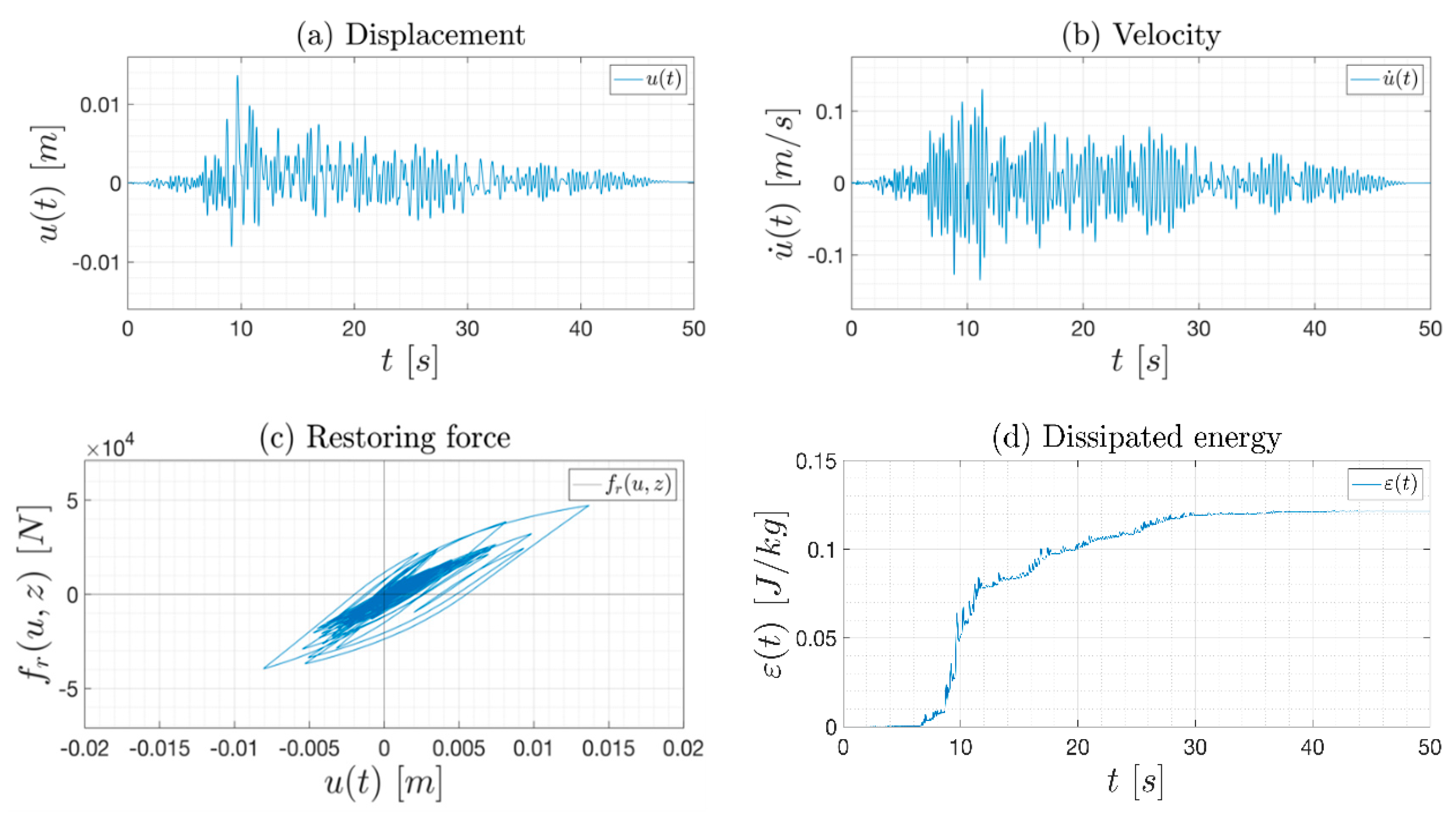
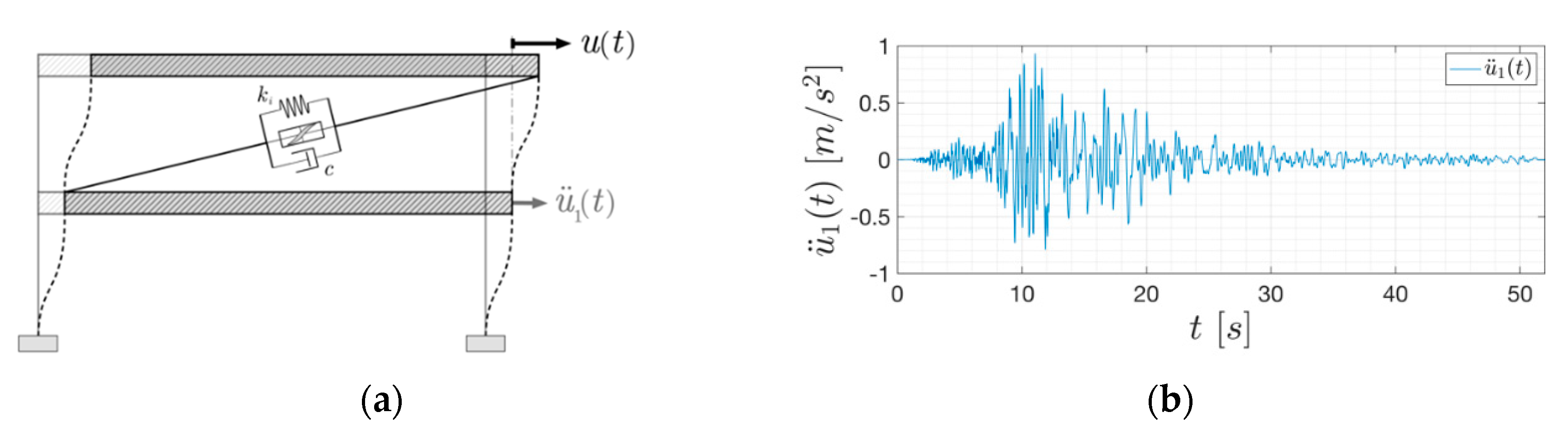
A record of the Montenegro earthquake (1979) was selected from the PEER Ground Motion Database (PEER, 2019) as seismic excitation (Figure 2) for the benchmark.
This input excitation was used to simulate the response of a SDoF Bouc–Wen–Baber–Noori (BWBN) nonlinear system with mass of m = 1200   kg and monitored by a dynamic monitoring system composed of one accelerometer installed on the system lumped mass. The initial stiffness k i of the system was calibrated with the objective of obtaining a plausible system frequency for a masonry structure of approximately 4   Hz . A damping ratio of ξ = 3 % was adopted according to relevant literature on masonry structures. Finally, the remaining BWBN parameters used to generate the simulated record are presented in Table 1, while Figure 3 depicts the simulation record data. The Bayesian calibration was then carried out on the simulated velocity response. The latter was chosen because it is simpler to describe such a system by a single ODE with respect to velocity. Deterministic values were set for the following parameters of the BWBN model: m = 1200   kg ,   A = 1 ,   N = 1 , and also for the damping ratio, ξ = 3 % . The latter assumption was made to release uncertainties related to the identification of ξ from the calibration process. Instead, the remaining ones were considered independent random variables with associated distributions given in Table 2 and constitute the vector of uncertain model parameters x M . It is worth specifying that the degradation effect of the BWBN model has been neglected on purpose, in order to introduce a discrepancy in the model used for emulating the reference response of the system. Besides, no uncertainties in input excitation have been considered herein, in order to address them only on the model side. The first moments of the prior probability density functions (PDFs) of model parameters k i and α, namely μ k i = 7.42 and μ α = 0.063 , were selected by two linear regressions on the reference restoring force curve for small and high displacements. The standard deviations of these parameters were chosen in order to take into account an amount of variation from these values of the 10%. It is worth noticing that in Table 2 a new random variable γ was introduced in order to guarantee the bounded-input, bounded-output (BIBO) stability [40]. Indeed, assuming as prior knowledge on the parameter γ the required BIBO stability condition (i.e., γ being uniformly distributed between the bounds β γ β ), the conditional distribution π ( γ | β ) must be uniform.
This can be achieved by transforming the input variables, namely removing the parameter γ and introducing an auxiliary variable γ U ( 1 , 1 ) . Hence, for a joint realization of the parameters β and γ , the actual parameter reads: γ   =   γ β for β 0 . The standard deviations of the latter parameters were computed trivially once the supports of the uniform distributions were defined. To infer the unknown residual variances σ 2 (Equation (9)), a uniform prior distribution was assumed:
π ( σ 2 ) U ( 0 , m a x | u ˙ | 2 ) ,
whose standard deviation was set equal to the maximum of the absolute value over the time of the experimental observation u ˙ 
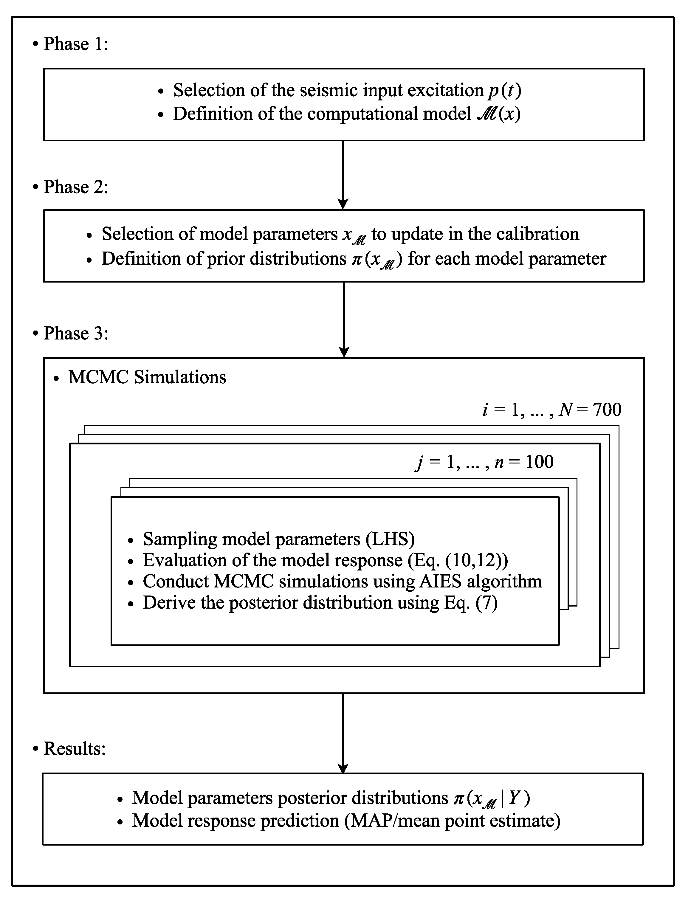
. Markov Chain Monte Carlo (MCMC) simulations have been conducted using MATLAB-based Uncertainty Quantification framework UQLab-V1.3-113® [6] with 100 chains, 700 steps and AIES solver algorithm [28]. The number of the BWBN forward model B W ( x ) calls in MCMC was 70′000. The system of ordinary differential equation (ODEs; Equations (10) and (12)) was solved with the MATLAB solver ode45 (explicit Runge–Kutta method with relative error tolerance 1 × 10
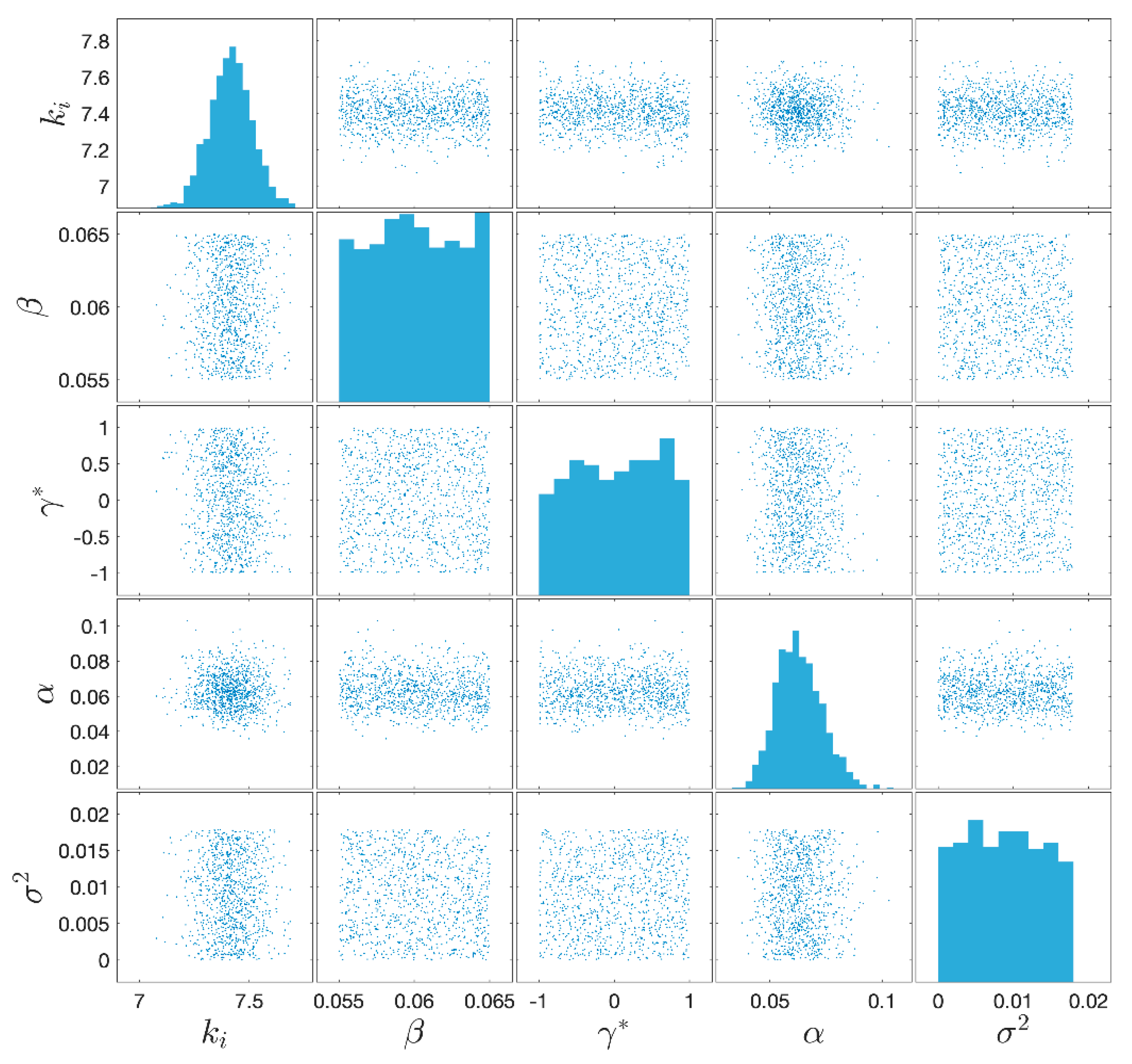
⁻³). The Latin hypercube sampling (LHS) method was used to get the parameters prior distributions (Table 2) of the BWBN model, which are shown in Figure 4.
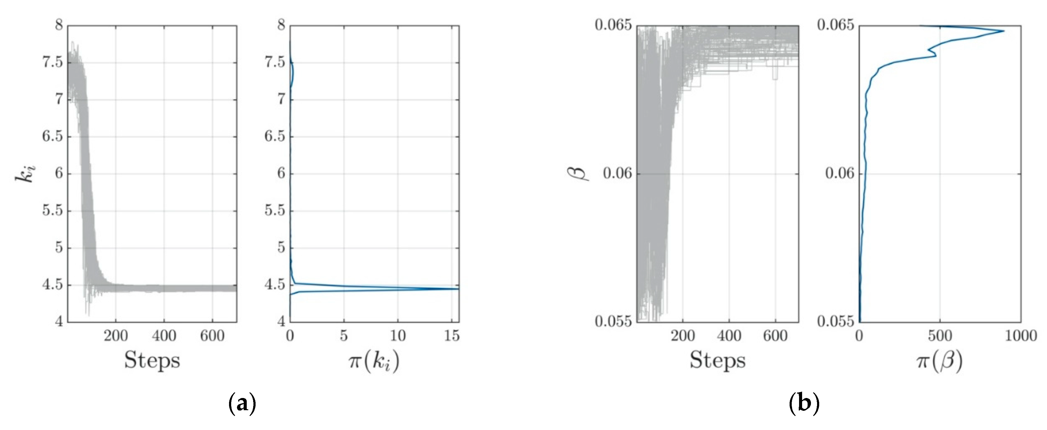
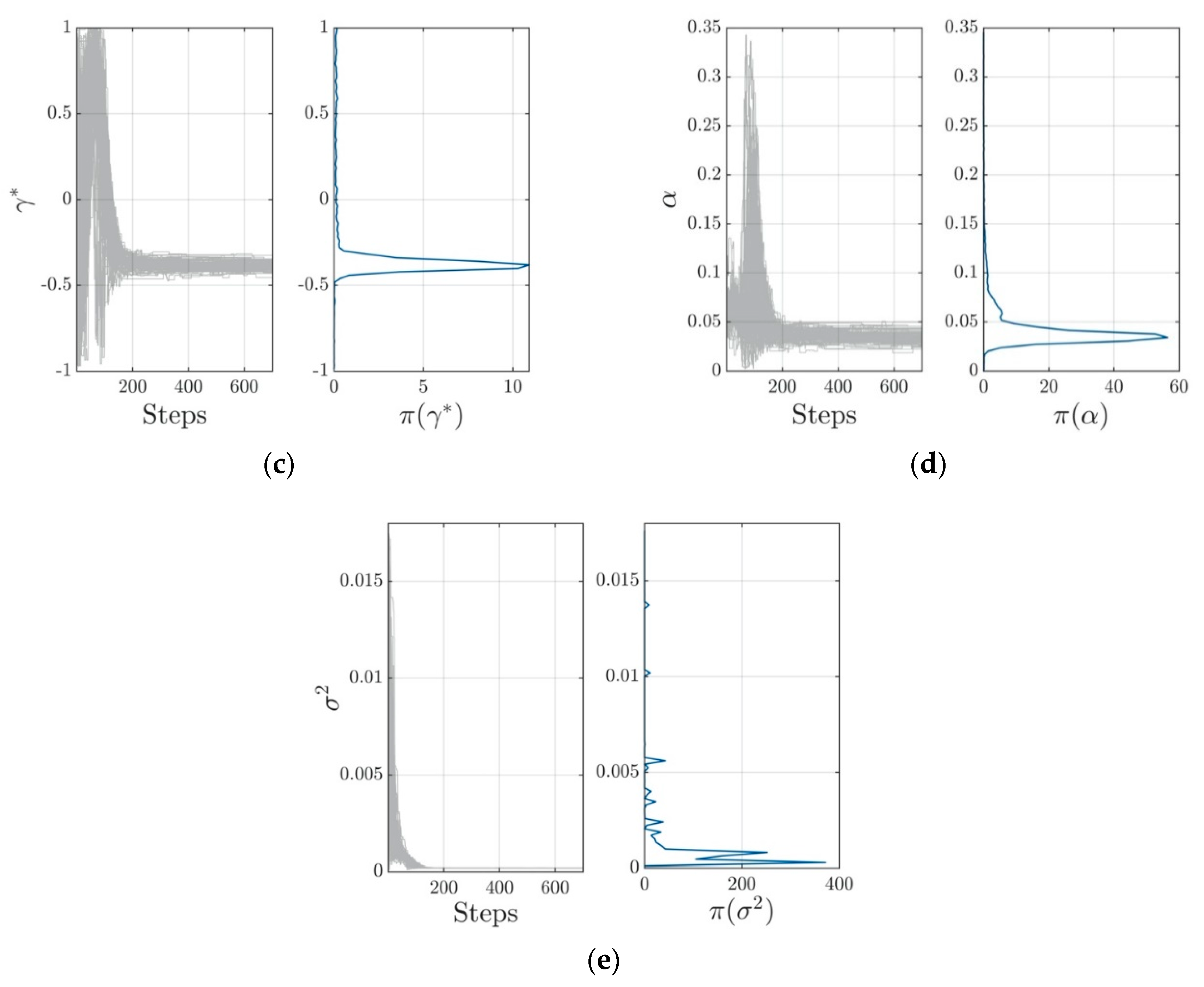
The evolutions of the Markov chains are plotted instead in Figure 5 for each model parameter x = { k i , β , γ , α , σ 2 } . These give valuable insights about convergence of the chains. Indeed, it can be clearly seen that 700 steps are sufficient to reach the steady state. Consequently, samples generated by the chains follow the posterior distributions. However, the sample points generated by the AIES MCMC algorithm have been post-processed carrying out the burn-in of the first half of sample points before convergence to avoid the pollution of the estimate of posterior properties. In our case, the quality of the generated MCMC chains can be judged satisfactory. Table 3 reports the result of the Bayesian inversion analysis: mean and standard deviation of the posterior 5%–95% quantiles of the distribution and Maximum A Posteriori (MAP) point estimate. The MAP can be assumed as the most probable parameter value following calibration. This value has been used as a best-fit parameter.
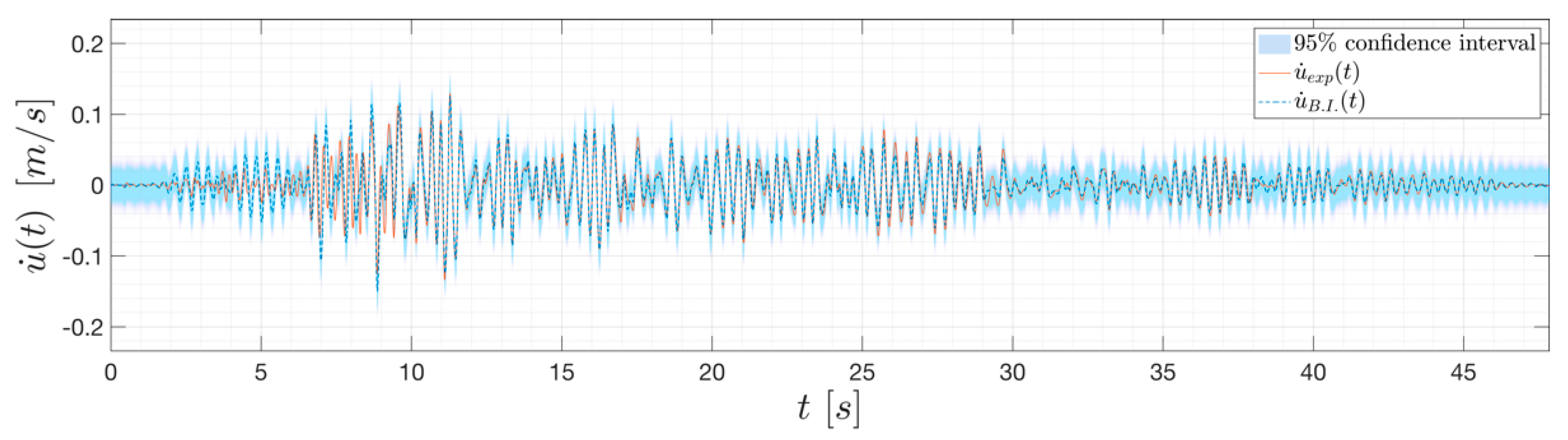
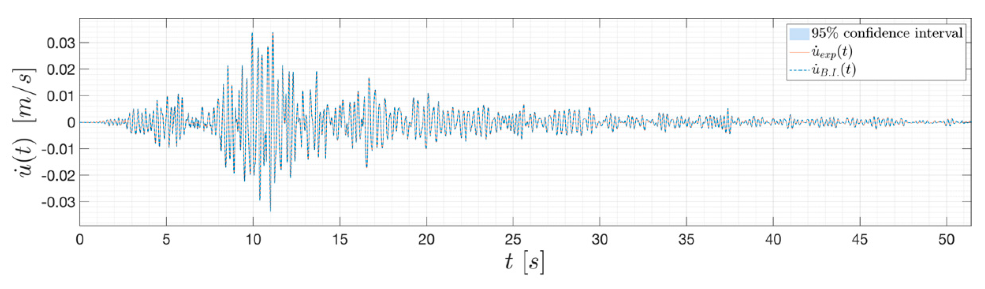
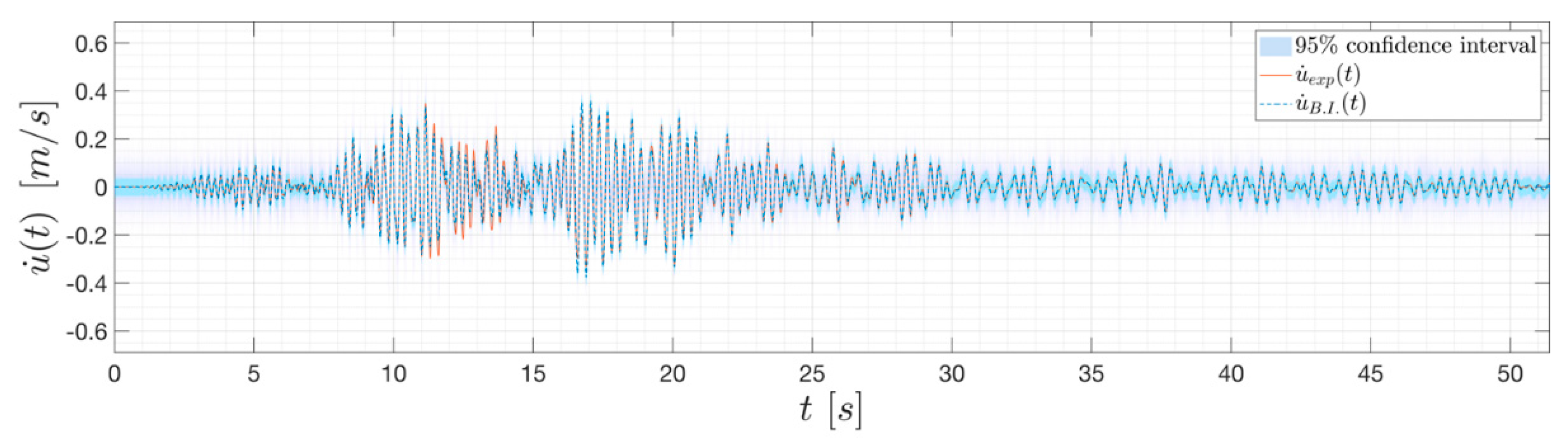
The model response prediction using MAP as a point estimate of the posterior distributions is plotted in Figure 6. It can be clearly seen how the inferred response reproduces the experimental record quite accurately, with a mean square error (MSE) over the time of 2.007 × 10⁻⁴ (i.e., half of the average of the MSE computed on all the post-predictive model runs, MSE = 4.0415 × 10⁻⁴). In fact, we should not dwell on this specific prediction; rather, we should consider its confidence intervals. The latter tells us how uncertainties on model input propagate through the model.
From inspection of 
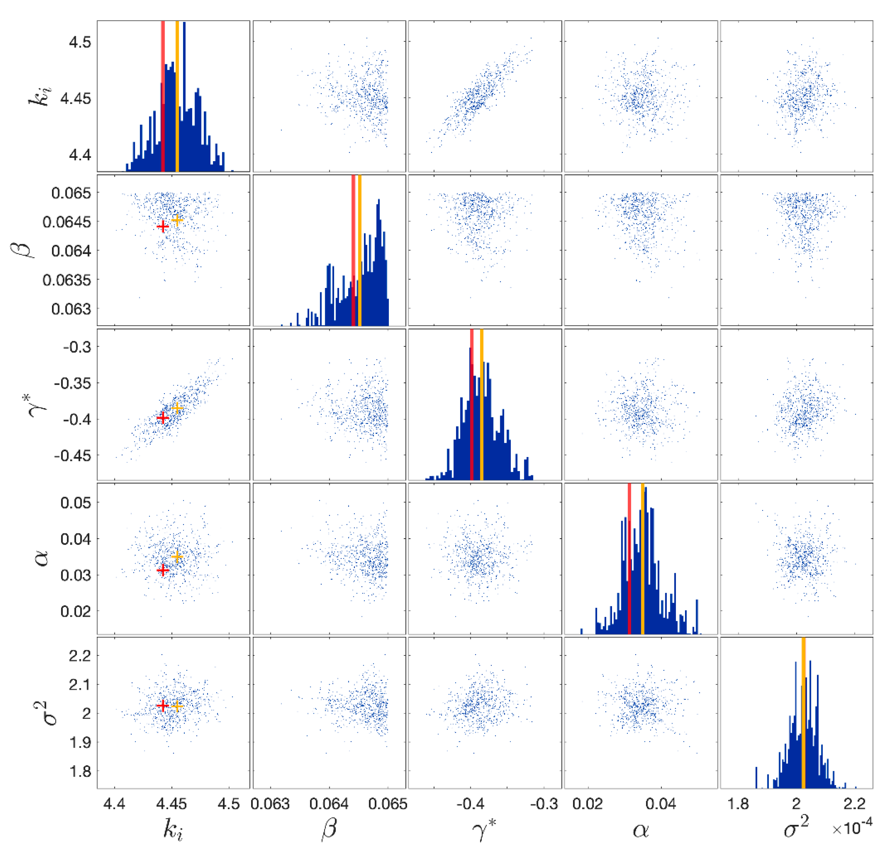
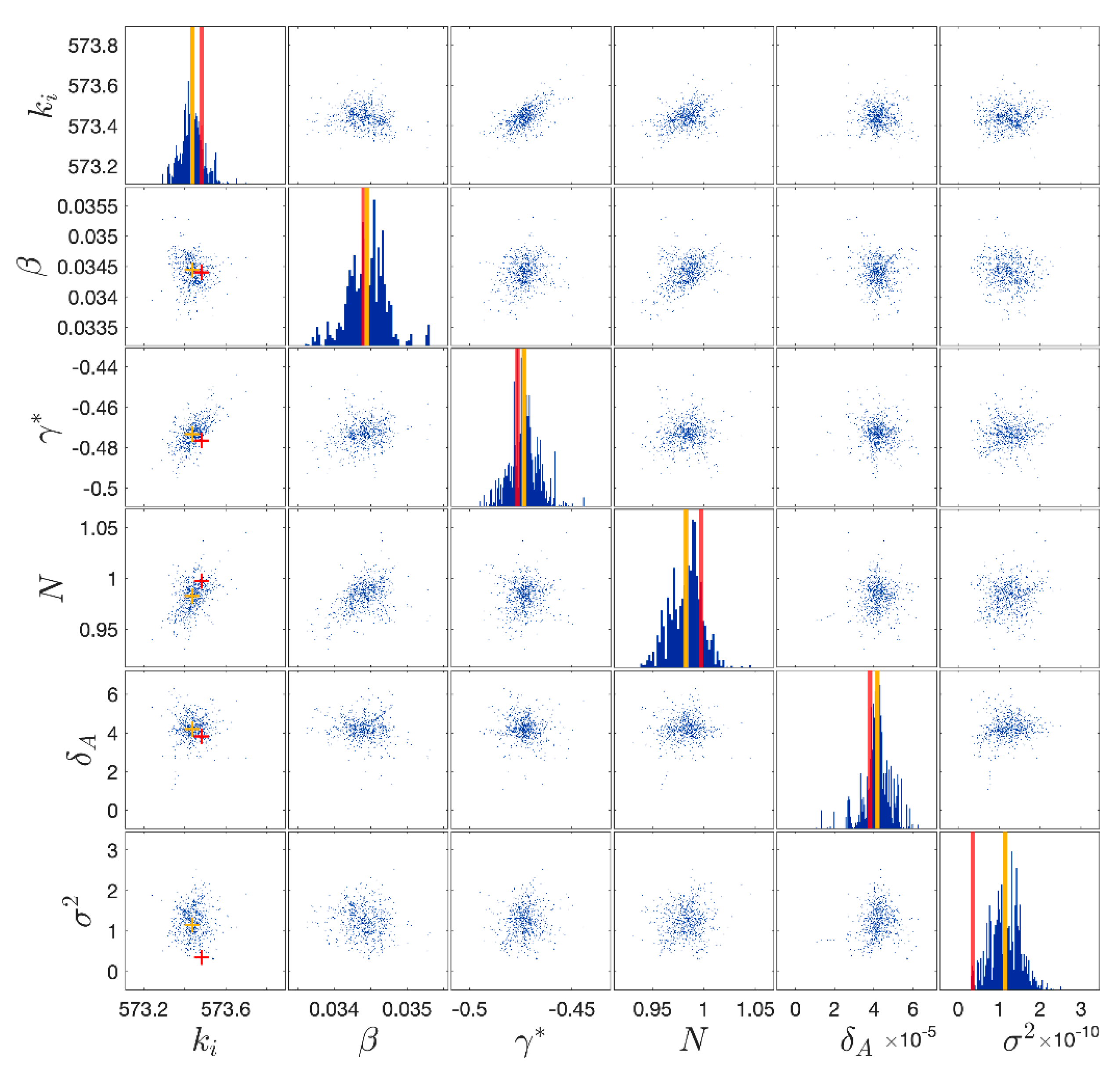
Figure 6 it can be concluded that uncertainties on the input parameters produce higher uncertainty of the response prediction in the lower amplitude regions rather than in the peak values. However, this is a satisfying result in earthquake engineering, where one is more interested in predicting maximum response quantities. The posterior distributions of the calibrated parameter are plotted in Figure 7.

3.2. Demonstration on a Case Study

Having established that the UQ framework can significantly help to gain insight into the uncertainties intrinsic to calibration, thus furnishing a realistic level of confidence on model prediction, this can now be applied to a case study. The aim is to study how the UQ works with an identified hysteretic and degrading model that emulates the experimental response of a real monitored masonry building, the Town Hall of Pizzoli, subjected to its real earthquake recorded data. This is a three-story stone masonry building located northwest of the city of L’Aquila (Abruzzo), which is away from the city. It was built around 1920 and it formerly hosted a school. The structure presents a u-shaped regular plan mainly distributed along one direction, and its elevations are characterized by regular openings distributed along three levels above the ground (the raised ground floor, the first floor and the under-roof floor). The total area is about 770 m2 while the volume is about 5000 m3. 
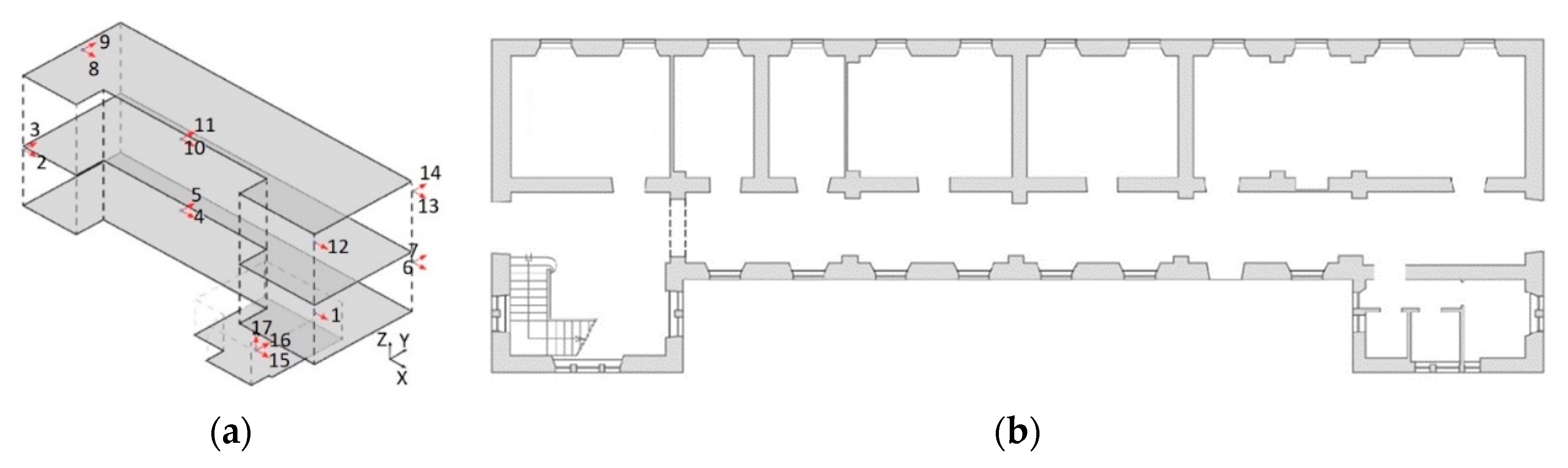
Figure 8 reports the schematizations of the analyzed building. The Town Hall of Pizzoli belongs to the network of buildings monitored by OSS [26]. The OSS monitors the structure of Pizzoli thanks to a dynamic monitoring system composed of eight accelerometers installed on the building and one placed in the basement. More specifically, a tri-axial accelerometer to record the seismic input in the three space directions is fixed in the basement. On the raised ground floor, no accelerometers are present. On the first floor, three biaxial accelerometers and one monoaxial accelerometer (in X direction) are present to capture the acceleration responses of the first floor in the two horizontal directions. Finally, the same scheme of sensors installed on the first floor is present on the second floor. It is worth noting that the acquisition system and the sensors setup was designed by OSS and represents an input data for our analyses. In this regard, to obtain an optimal positioning of the sensors, a finite element model should be used. In particular, the optimal sensor placement is done recurring to a linear finite element model (using eigen-analysis, singular value decomposition, etc.). The model is often linear to perform this task because for nonlinear analysis the linear elastic component commonly brings the predominant amount of the output variance.
The system sampled the signals at 250 Hz, for a total duration of about 50 s for the analyzed earthquake. The acquisition system recorded the sequence that struck central Italy in 2016. For this study, the earthquake acceleration responses of the building recorded on 30 October 2016 were used as reference signals. It is worth noting that accelerometric data are used in this work to define the likelihood function during the calibration. This is true as the use of inter-storey drift in the definition of the likelihood function would require its estimation. This estimate is often complicated because the filtering and integration operation on experimental data usually brings errors during the elaboration, especially with respect to the time alignment of two different recorded signals (quantities that are needed to estimate the inter-storey drift).
Since the scope of this study is to show how the discrepancy of models affects the calibration of model parameters value for seismic SHM, only the inter-storey response of the under-roof floor (2nd DoF) has been considered as reference output quantity. The acceleration of the first floor (1st DoF) is considered as the input signal of the reference model. The decision to use an inter-storey law is based on the fact that the results of the calibration will be compared with the results of calibration performed with discrepant models. In this sense, a single DoF model helps to make a direct comparison of the results, since the correspondence of parameters belonging to different models becomes less obvious for multi DoF models. The idea is to present a numerical case study derived from a real-world structure, with realistic values for hysteretic model parameters.

3.2.1. Reference Model

In this subsection, the model that came as the result of a nonlinear identification previously performed on the Pizzoli Town Hall structure is described for completeness. The nonlinear identification, like in [41,42], relied on a plane frame model in the direction of minor inertia of the building. Assuming the mass contribution of the raised ground floor in the dynamics of the structure is negligible, the building has been modelled with two lumped masses in correspondence to the first and under-roof floor.
The identification procedure consisted of using absolute acceleration data measured at the floors to approximate the response with a generalized linear model obtained by expanding the Bouc–Wen model of hysteresis.
The basic functions of the generalized linear model ended up being nonlinear in terms of the exponential parameters of the BW model. These parameters were therefore identified with specialized optimization algorithms, while for the remaining parameters a direct estimate in the joint time-frequency domain was performed. The identification provided also instantaneous values of the BW model parameters made explicit by the generalized linear model. The main findings of the identification can be summarized as follow:
  • The adopted procedure allowed verification of the consistency of the assumed nonlinear model. This was done by checking the stability of the values of the model parameters over time.
  • The resulting model satisfactorily reproduced the experimental response. This was validated in [43] by comparing the model results with the experimental findings obtained by the authors and by other researchers [44] independently,
  • The procedure allowed for the collection of timely information on the health of the structure immediately after the occurrence of the earthquake.
In the identification process, a global box-like behavior was assumed, also based on the results of on-site inspections that led to the verification of the existence of good connections between walls and floor-walls before the occurrence of seismic events. In addition, no strength deterioration was accounted for (i.e., ν ( ε h ) = 1 ), while for the stiffness degradation, only the proportional component was maintained (i.e., η ( ε h ) = 1 and A ( ε h ) = 1 δ A ε h ( t ) ) . The parameter α was instead imposed to zero. These choices were made to make the reference model consistent with the model identified in [43], which was calibrated with experimental data.
The reference two DoFs model has been reconducted to a DoF by imposing the acceleration response of the first floor of the Town Hall (recorded by the monitoring system), u ¨ 1 ( t ) , as the input signal. The output was obtained for the inter-story drift, u ( t ) , between the under-roof and the first floor. For further information on the identified model one can refer to [43].
Thus, the reference model used for the analysis from now on becomes:
m · u ¨ ( t ) + f ( t ) = m · u ¨ 1 ( t ) ;
f ˙ L ( t ) = k ( ε h ( t ) , t ) · u ˙ ( t ) ;
k ( ε h ( t ) , t ) = k i · ( 1 δ A · ε h ( t ) ) = k i k i δ A · ε h ( t ) ;
f ˙ N L ( t ) = β u ˙ ( t ) | f ( t ) | N s i g n [ u ˙ ( t ) f ( t ) ] γ u ˙ | f ( t ) | N .
The reference model is depicted in Figure 9 with the acceleration input u ¨ 1 ( t ) , while the corresponding model parameters, identified in a previous study with the Pizzoli Town Hall building responses, are reported in Table 4. For the numerical simulations, a viscous damping term (with a damping ratio of 3% set as a deterministic value in the calibration process) has been added to the model of Equation (16).

3.2.2. Bayesian Calibration of the Reduced Single DoF Reference Model

The reduced single DoF BWBN model was used to validate the entire procedure in the first phase. Table 5 and Table 6 report the prior information on model parameters and the results of the Bayesian inversion, respectively. Figure 10 depicts the posterior distributions of the parameters, while Figure 11 depicts the velocity response of the oscillator once the model has been calibrated. From the inspection of the latter, it can be concluded that uncertainties on the input parameters do not affect the response prediction.
Moreover, the value of the degrading term δ A turns out not to influence the response prediction. This is due to the fact that during the earthquake shaking (PGA 1 m/s2) the structure exhibited a low level of damage [44].
Both parametric and non-parametric degradation models have been used herein. Two models per each family are first mathematically introduced, then insights into the accuracy afforded by each model are provided.

3.2.3. Models for Stiffness Degradation

Besides the original BWBN degrading model, an additional parametric model is now introduced to investigate the capability of the Gaussian model discrepancy term to cover model uncertainty. An important part of the current literature on damage indices focuses on exponential function of the dissipated energy.
Consequently, an energy-based exponential function, according to [45], has been used in this work to replace the original BWBN stiffness degradation term ( 1 δ A ε ( t ) ) that multiplies the initial stiffness k i :
D E ( t , ε , β ) = exp ( β ε ( t ) ( m u ¨ m a g ) d t ) ,
where β is an additional parameter to infer jointly with k i . In order to replicate the degrading effect on the initial stiffness k i through non-parametric models, probability distribution functions have been used herein. First, according to the procedure used in [46], a Weibull distribution function was adopted:
D W ( t , R W , p 1 , p 2 ) = ( 1 [ R W R W   e x p ( t p 1 ) p 2 ] ) ,
where R ,   p 1 ,   p 2 are the distribution parameters to infer jointly with k i . Meaning to these parameters may be given as follows: p 1 represents the instant of time at which there is loss of stiffness; p 2 controls its rate; and RW controls the amount of damage. Secondly, a logistic distribution function was adopted:
D L ( t , R L , μ , s ) = ( 1 R L 1 + e x p ( t μ s ) ) .
In this case, parameter μ is the instant of time in which the loss of stiffness occurs, while parameter s represents its rate, and RL defines the amount of degradation.

3.2.4. Comparison of the Calibrated Models

It is useful to make a comparison among all the models introduced to get insights on their accuracy in predicting the response of the oscillator. For the sake of simplicity, from now Model 1, Model 2, Model 3 and Model 4 will refer to the models with the degrading law of the original BWBN model, the exponential law, the Weibull and the logistic distribution functions, respectively. It is also worth noticing that, in order to reduce the number of parameters to infer, only the initial stiffness k i and the degrading term have been involved in the calibration process. This can be easily justified by the fact that, for practical earthquake engineering applications, the focus relies on the quantification of the structure’s stiffness and its drop (especially for masonry structures which are prone to crack during a seismic event). Prior information on the possible value of the model parameters was obtained by visual inspection of the dissipated energy versus time curve. For both parametric and non-parametric models, the velocity response of the system obtained was almost identical to Figure 11 for a low-level of degradation. 
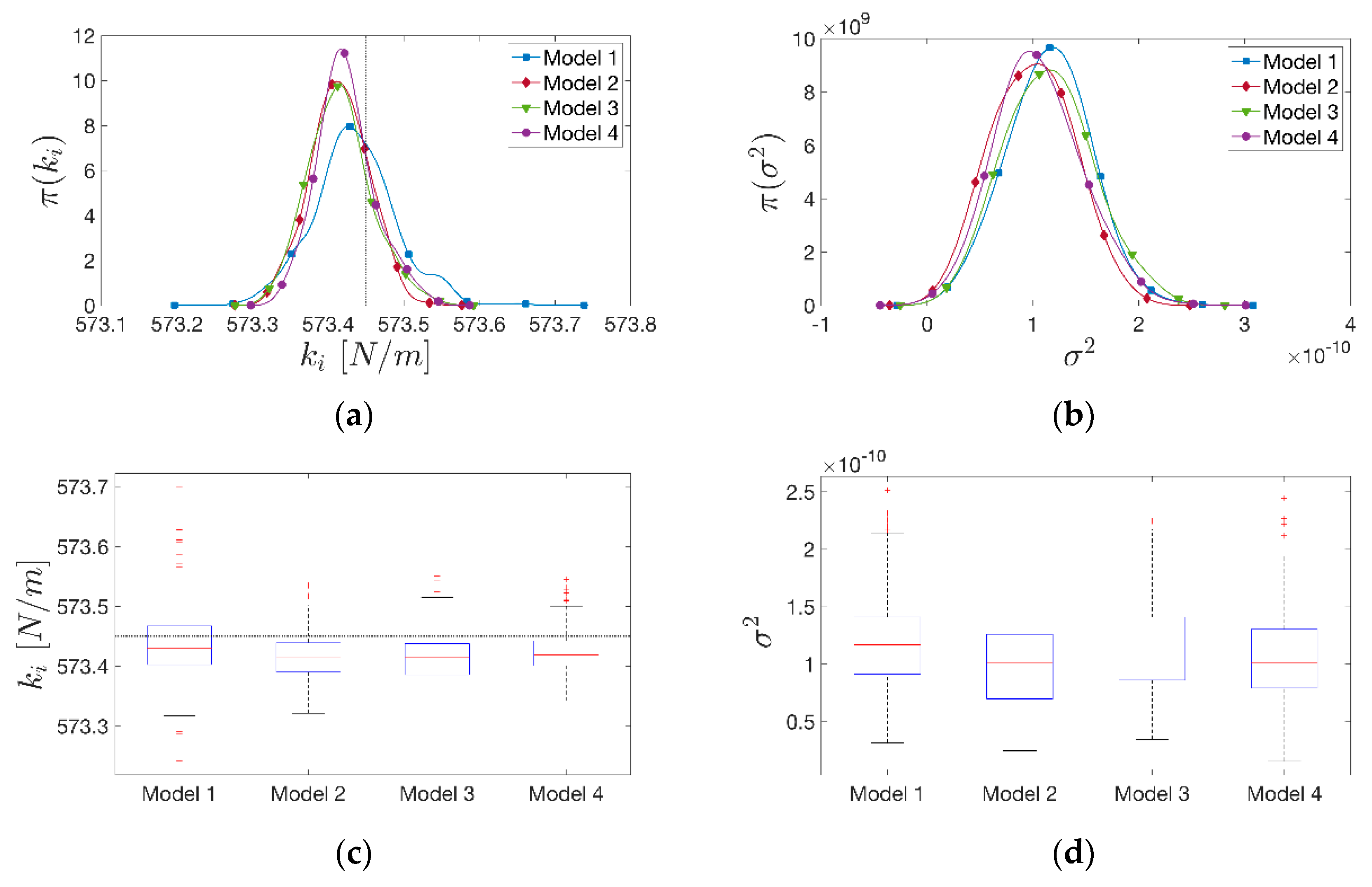
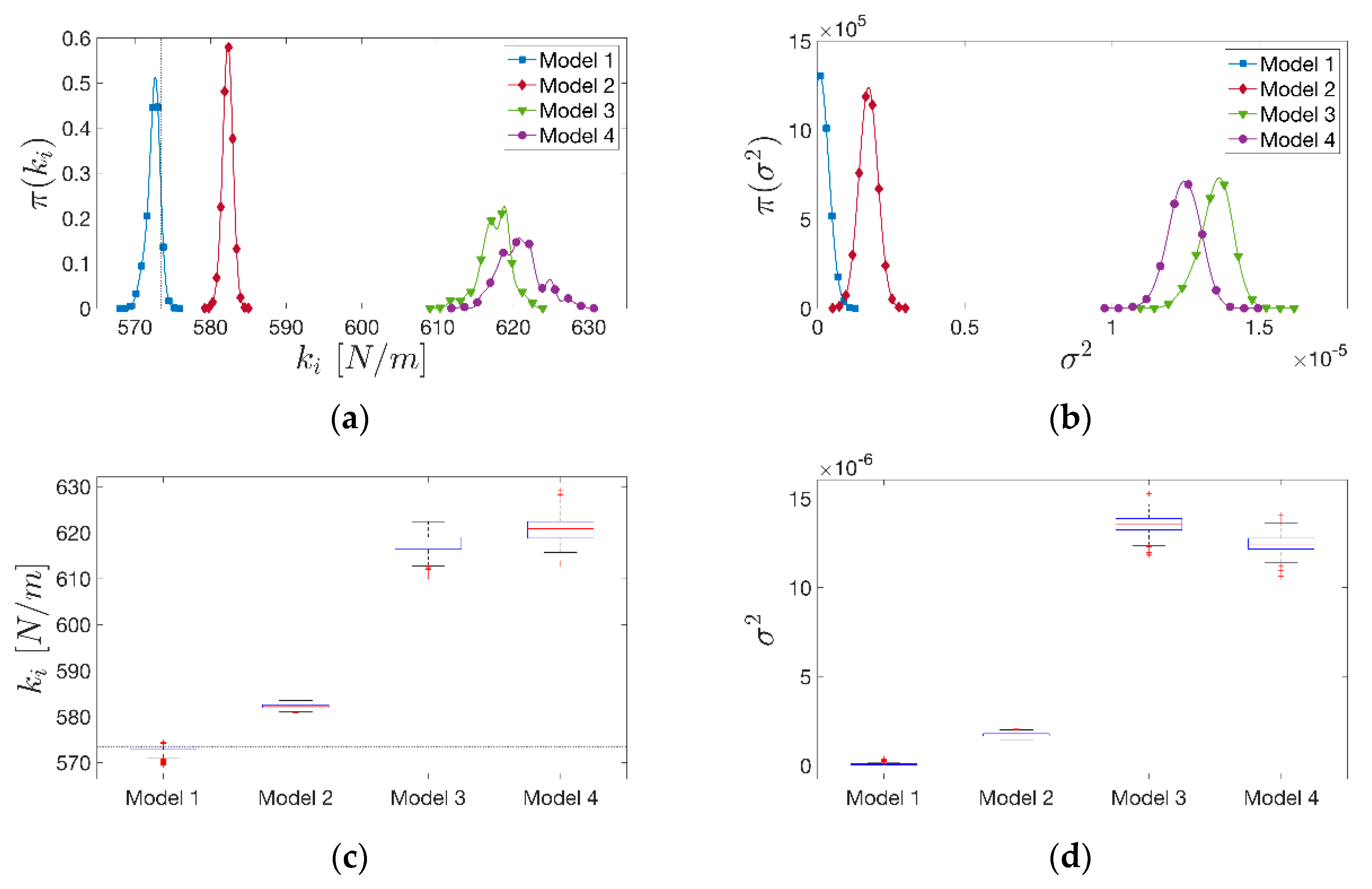
Figure 12 depicts the posterior distributions of the initial stiffness parameter k i for each model considered. From this inspection, it can be seen that all models were able to predict the correct value of the initial stiffness. The choice of the MAP (or of the mean of the distributions) as a point estimate after the uncertainty propagation led to a slightly underrated initial stiffness regardless of the model adopted. However, this is neglectable from an engineering point of view. Moreover, Figure 12 depicts the distributions of the discrepancy variance term σ 2 as well. All the models share the same order of magnitude for σ 2 and, more or less, the same variance. This can be read as follows: the adopted Gaussian discrepancy term, with mean null and unknown variance, performs as a good function to embody all the model errors arising. Thus, at the end, it appears clear how the choice of the model used to infer the stiffness of the oscillator is not meaningful in the presence of a low-level of damage.

3.3. Influence of the Degradation Level on Model Parameters Inference

Having established that the choice of the models used to infer the stiffness parameter k i appears to not be relevant for a low-level of degradation, the aim is now to investigate what happens in possible further scenarios in which a higher level of damage is exhibited. This study is important when working in the field of model calibration because it explains the importance of linking the choice of the discrepancy model distribution—which is needed as input in the calibration process—to the degradation amount and the characteristics of the external force (e.g., amplitude and frequency).
To this aim, the input excitation was rescaled. Specifically, two cases are examined as follows: (i) one in which the input has been rescaled with a PGA of 6 m/s2 (medium level of degradation); (ii) one in which the input has been rescaled with a PGA of 9 m/s2 (high level of degradation).

3.3.1. Medium Level of Degradation

When increasing the level of excitation to a medium value (i.e., PGA of 6 m/s2) and keeping the same reference damage, all the models were still able to predict the correct value of the initial stiffness k i . However, an increase of the uncertainties in the model prediction was registered, this time due to the greater values of the discrepancy variance. The choice of the MAP (or of the mean of the distributions) as point estimate led to a slight overrating of the initial stiffness. As the estimation error was negligible, the adopted discrepancy term still performs as a good function to embody all the model errors. However, increasing the level of the input without accounting for a growth of the damage level appears to be unrealistic. This is because higher seismic excitations generally involve greater dissipation of energy. Therefore, a loss up to 40% of the initial stiffness k i was taken into account as well, resulting in Model 1 (i.e., the one consistent with the BWBN degrading model, which is able to predict the correct value of the initial stiffness). On the contrary, all the models inconsistent with the BWBN model (i.e., Models 2, 3 and 4) overrate the initial stiffness value in a non-negligible proportion (Figure 13), leading to higher level of uncertainty in the model response prediction. It is also worth noticing how the estimation error was amplified for non-parametric models. This is a considerable indicator of the inadequacy of the discrepancy function adopted. In order to recover the response records, more accurate and well-suited discrepancy models should be investigated, but this is beyond the scope of this paper.

3.3.2. High Level of Degradation

The final step consisted of increasing the level of input to a high value (i.e., PGA of 9 m/s2). Again, when keeping the same level of reference damage, all models were able to predict the correct value of the initial stiffness although with a visibly greater variance than before. When the level of damage increased, taking into account a stiffness loss of up to the 80% of the initial one, the same conclusions made in Section 3.3.1 were also confirmed, stressing the fact that level of uncertainty is now greater due to both greater excitation and a higher level of damage (Figure 14).

4. Discussion

This realistic case study has shown that a Gaussian discrepancy term, with null mean and unknown variance, is an effective choice to tackle the model inaccuracy rising for low levels of degradation when the aim is inference of the system’s initial stiffness. At the same time, it has been proven that this kind of discrepancy still works fine for low levels of damage even if the input is rescaled up to 1 g. Consequently, the discrepancy term adopted can be judged suitable to cover model errors with increasing values of the PGA. However, higher levels of PGA introduce higher uncertainties in the model prediction. It has been shown that increasing the amount of degradation jointly to the level of damage leads to inaccurate predictions for those models that are inconsistent with the original physical BWBN model and more uncertainty also arises in the latter. This can be appreciated, for example, in the velocity response prediction of Model 3 (Figure 15). This is the model that leads to the worst model prediction for high level of degradation, owing to the presence of a greater number of overestimated outliers.
What has been determined can be easily read from the graphs in Figure 16. The latter depicts the MSE error over the time of the velocity response prediction for each case. Specifically, Figure 16a–c display the variation of MSE computed for all the post-predictive model runs, for each model and for each level of degradation (low, medium and high). Instead, the comparison between the average MSE computed on all the post-predictive models runs versus the MSE of the MAP estimate prediction at different levels of degradation, is presented in Figure 16d. From the inspection of latter, we can conclude how the error in prediction increases as the level of degradation increases. This leads to more uncertain predictions.
At last, for those cases inconsistent with the physics model that presents from a medium to high level of damage, it can be concluded that the simple discrepancy function adopted is not sufficient to embody all the model errors. This means that the choice of the discrepancy function should be linked to the level of damage and, in actual practice applications, to the level of excitation.
Thus, to summarize the considerations on the use of Bayesian updating and the uncertainty quantification framework, one can state that the model errors and the observation errors can be taken into account by adding a discrepancy term in the model calibration process. This brings benefits in terms of calibration outcomes (i.e., in addition to good time-series fitting, the order of the parameters is close to the real value). However, for some cases, the Bayesian approach within the uncertainty quantification framework could bring trivial results in terms of model parameter values. This especially occurs if the discrepancy model distribution is not chosen properly. The findings of this paper show that a good way to choose the discrepancy model distribution could be to study potential correlations between it and the statistical nature of the external force (e.g., amplitude and frequency) and the statistical nature of the modal characteristics (e.g., natural frequencies) of a system, evaluated in operational conditions. For example, for external forces with frequency content close to the natural frequencies of the system, there is a high chance of high degradation to occur, and thus a discrepancy model distribution close to a Gaussian distribution could bring trivial results. This is clearly valid for a given model, since the model selection framework is another research topic that was not evaluated in this study and is complementary to the actual work.
This finding could stimulate further research on the statistical correlation of discrepancy models and the magnitude of excitation, helping to calibrate mathematical models that try to emulate real word systems and structures.

5. Conclusions

This article addressed the Bayesian probabilistic calibration of nonlinear hysteretic systems for model-driven seismic SHM purposes. The well-known Bayesian inversion framework was first illustrated through a numerical benchmark of a SDOF Bouc–Wen type oscillator, and then applied to a reference model derived from a calibrated 2-DOFs system of a real monitored masonry building hit by the 2016 Central Italy earthquake. The main novelty of this study is the application of this framework on models representing data measured directly on masonry structures during seismic events. In the examined cases, the model calibration procedures was carried out by incorporating the posterior uncertainty linked to model discrepancy in order to:
(i)
explicitly define the errors and uncertainties present in the model;
(ii)
provide the full multivariate distribution of the calibrated parameters;
(iii)
estimate the model discrepancy posterior distribution;
(iv)
provide insights on quantities of interest (e.g., maximum a posteriori estimates, time-history response prediction).
Furthermore, the study points to the importance of choosing a discrepancy model function correlated to the underlying seismic characteristics. This consideration can be drawn from the results obtained for the case study associated to Pizzoli Town Hall, for which several parametric and non-parametric degrading models were investigated to gain insight into how model inaccuracy could be embodied by the discrepancy function adopted. Specifically, with reference to non-parametric models, it has been determined that:
(i)
for low level of damage, and even for high levels of PGA, accurate predictions can be achieved adopting a Gaussian discrepancy term with null mean and unknown variance, which overcomes the low sensitivity of the term used to model the degradation in the response;
(ii)
for high levels of damage, on the contrary, the simple Gaussian discrepancy function is unable to tackle the model inaccuracy rising.
This means that, when the magnitude of the external excitation is very high (for the system considered), or the system is subjected to resonance, the system is likely to undergo damage (e.g., to high level of degradation) and thus simplified assumptions on the model discrepancy term are not reasonable. For these cases, the use of a fuller and more specific model for the mean of the discrepancy term should be used to get reliable estimates. These results suggest further studies to better relate discrepancy models to the statistical nature of the excitation and other factors that can influence probabilistic model calibration for use in seismic SHM.

Author Contributions

Methodology, A.F.; case study, A.F. and G.M.; review, R.C. and G.M., editing, A.F.; supervision, R.C. All authors have read and agreed to the published version of the manuscript.

Funding

This research received no external funding.

Acknowledgments

The data of the Town Hall of Pizzoli were supplied by the Seismic Observatory of Structures within the DPC-ReLUIS project. Computational resources were provided by HPC@POLITO (http://hpc.polito.it).

Conflicts of Interest

The authors declare no conflict of interest.

References

  1. Biegler, L.; Biros, G.; Ghattas, O.; Heinkenschloss, M.; Keyes, D.; Mallick, B.; Tenorio, L.; van Bloemen Waanders, B.; Willcox, K.; Marzouk, Y. Large-Scale Inverse Problems and Quantification of Uncertainty; Wiley Online Library: Hoboken, NJ, USA, 2011; Volume 712. [Google Scholar]
  2. Bernagozzi, G.; Mukhopadhyay, S.; Betti, R.; Landi, L.; Diotallevi, P.P. Output-only damage detection in buildings using proportional modal flexibility-based deflections in unknown mass scenarios. Eng. Struct. 2018, 167, 549–566. [Google Scholar] [CrossRef]
  3. Liu, Y.; Mei, Z.; Wu, B.; Bursi, O.S.; Dai, K.-S.; Li, B. Seismic behaviour and failure-mode-prediction method of a reinforced-concrete rigid-frame bridge with thin-walled tall piers: Investigation by model-updating hybrid test. Eng. Struct. 2020, 208, 110302. [Google Scholar] [CrossRef]
  4. Moon, F.; Catbas, N. Structural Identification of Constructed Systems: Approaches, Methods, and Technologies for Effective Practice of St-Id; American Society of Civil Engineers (ASCE): Reston, WV, USA, 2013. [Google Scholar] [CrossRef] [Green Version]
  5. Beck, J.L.; Katafygiotis, L.S. Updating Models and Their Uncertainties. I: Bayesian Statistical Framework. J. Eng. Mech. 1998, 124, 455–461. [Google Scholar] [CrossRef]
  6. Wagner, P.-R.; Nagel, J.; Marelli, S.; Sudret, B. UQLab User Manual—Bayesian Inversion for Model Calibration and Validation; Chair of Risk, Safety and Uncertainty Quantification: ETH Zurich, Switzerland, 2019. [Google Scholar]
  7. Noel, J.; Kerschen, G. Nonlinear system identification in structural dynamics: 10 more years of progress. Mech. Syst. Signal Process. 2017, 83, 2–35. [Google Scholar] [CrossRef]
  8. Ching, J.; Beck, J.L.; Porter, K.A. Bayesian state and parameter estimation of uncertain dynamical systems. Probabilistic Eng. Mech. 2006, 21, 81–96. [Google Scholar] [CrossRef]
  9. Ortiz, G.A.; Alvarez, D.A.; Bedoya-Ruiz, D. Identification of Bouc–Wen type models using the Transitional Markov Chain Monte Carlo method. Comput. Struct. 2015, 146, 252–269. [Google Scholar] [CrossRef]
  10. Chen, H.-P.; Mehrabani, M.B. Reliability analysis and optimum maintenance of coastal flood defences using probabilistic deterioration modelling. Reliab. Eng. Syst. Saf. 2019, 185, 163–174. [Google Scholar] [CrossRef]
  11. Erazo, K.; Nagarajaiah, S. An offline approach for output-only Bayesian identification of stochastic nonlinear systems using unscented Kalman filtering. J. Sound Vib. 2017, 397, 222–240. [Google Scholar] [CrossRef]
  12. Zhou, K.; Tang, J. Uncertainty quantification in structural dynamic analysis using two-level Gaussian processes and Bayesian inference. J. Sound Vib. 2018, 412, 95–115. [Google Scholar] [CrossRef]
  13. Yan, G.; Sun, H. A non-negative Bayesian learning method for impact force reconstruction. J. Sound Vib. 2019, 457, 354–367. [Google Scholar] [CrossRef]
  14. Yan, W.-J.; Chronopoulos, D.; Papadimitriou, C.; Cantero-Chinchilla, S.; Zhu, G.-S. Bayesian inference for damage identification based on analytical probabilistic model of scattering coefficient estimators and ultrafast wave scattering simulation scheme. J. Sound Vib. 2020, 468, 115083. [Google Scholar] [CrossRef]
  15. Imholz, M.; Faes, M.; Vandepitte, D.; Moens, D. Robust uncertainty quantification in structural dynamics under scarse experimental modal data: A Bayesian-interval approach. J. Sound Vib. 2020, 467, 114983. [Google Scholar] [CrossRef]
  16. Hizal, Ç.; Turan, G. A two-stage Bayesian algorithm for finite element model updating by using ambient response data from multiple measurement setups. J. Sound Vib. 2020, 469, 115139. [Google Scholar] [CrossRef]
  17. Muto, M.; Beck, J.L. Bayesian Updating and Model Class Selection for Hysteretic Structural Models Using Stochastic Simulation. J. Vib. Control. 2008, 14, 7–34. [Google Scholar] [CrossRef] [Green Version]
  18. Wu, M.; Smyth, A.W. Application of the unscented Kalman filter for real-time nonlinear structural system identification. Struct. Control. Health Monit. 2007, 14, 971–990. [Google Scholar] [CrossRef]
  19. Astroza, R.; Ebrahimian, H.; Conte, J. Material Parameter Identification in Distributed Plasticity FE Models of Frame-Type Structures Using Nonlinear Stochastic Filtering. J. Eng. Mech. 2015, 141, 04014149. [Google Scholar] [CrossRef]
  20. Conte, J.; Astroza, R.; Ebrahimian, H. Bayesian Methods for Nonlinear System Identification of Civil Structures. In Proceedings of the MATEC Web Conference, Zürich, Switzerland, 19–21 October 2015; Volume 24, p. 03002. [Google Scholar] [CrossRef]
  21. Jalayer, F.; Iervolino, I.; Manfredi, G. Structural modeling uncertainties and their influence on seismic assessment of existing RC structures. Struct. Saf. 2010, 32, 220–228. [Google Scholar] [CrossRef]
  22. Gardoni, P.; Der Kiureghian, A.; Mosalam, K.M. Probabilistic Capacity Models and Fragility Estimates for Reinforced Concrete Columns based on Experimental Observations. J. Eng. Mech. 2002, 128, 1024–1038. [Google Scholar] [CrossRef]
  23. Bracchi, S.; Rota, M.; Magenes, G.; Penna, A. Seismic assessment of masonry buildings accounting for limited knowledgeon material by Bayesian updating. Bull. Earthq. Eng. 2016, 14, 2273–2297. [Google Scholar] [CrossRef]
  24. Ramos, L.F.; Miranda, T.; Mishra, M.; Fernandes, F.; Manning, E. A Bayesian approach for NDT data fusion: The Saint Torcato church case study. Eng. Struct. 2015, 84, 120–129. [Google Scholar] [CrossRef] [Green Version]
  25. Bartoli, G.; Betti, M.; Facchini, L.; Marra, A.; Monchetti, S. Bayesian model updating of historic masonry towers through dynamic experimental data. Procedia Eng. 2017, 199, 1258–1263. [Google Scholar] [CrossRef]
  26. Dolce, M.; Nicoletti, M.; De Sortis, A.; Marchesini, S.; Spina, D.; Talanas, F.; De Sortis, A. Osservatorio sismico delle strutture: The Italian structural seismic monitoring network. Bull. Earthq. Eng. 2015, 15, 621–641. [Google Scholar] [CrossRef] [Green Version]
  27. Marelli, S.; Sudret, B. UQLab: A Framework for Uncertainty Quantification in Matlab. Vulnerability Uncertain. Risk 2014, 2554–2563. [Google Scholar] [CrossRef] [Green Version]
  28. Goodman, J.; Weare, J. Communications in Applied Mathematics and Computational Science; Math. Sci. Publishing: Berkeley, CA, USA, 2010. [Google Scholar]
  29. Kyprianou, A.; Worden, K.; Panet, M. Identification Of Hysteretic Systems Using The Differential Evolution Algorithm. J. Sound Vib. 2001, 248, 289–314. [Google Scholar] [CrossRef]
  30. Worden, K.; Hensman, J. Parameter estimation and model selection for a class of hysteretic systems using Bayesian inference. Mech. Syst. Signal Process. 2012, 32, 153–169. [Google Scholar] [CrossRef]
  31. Ben Abdessalem, A.; Dervilis, N.; Wagg, D.J.; Worden, K. Model selection and parameter estimation in structural dynamics using approximate Bayesian computation. Mech. Syst. Signal Process. 2018, 99, 306–325. [Google Scholar] [CrossRef]
  32. Ceravolo, R.; Demarie, G.V.; Erlicher, S. Instantaneous Identification of Degrading Hysteretic Oscillators Under Earthquake Excitation. Struct. Health Monit. 2010, 9, 447–464. [Google Scholar] [CrossRef]
  33. Ceravolo, R.; Demarie, G.V.; Erlicher, S. Instantaneous Identification of Bouc-Wen-Type Hysteretic Systems from Seismic Response Data. Key Eng. Mater. 2007, 347, 331–338. [Google Scholar] [CrossRef] [Green Version]
  34. Ceravolo, R.; Demarie, G.V.; Erlicher, S. Identification of degrading hysteretic systems from seismic response data. In Proceedings of the 7th European Conference on Structural Dynamics, EURODYN 2008, Leuven, Belgium, 20–22 September 2008. [Google Scholar]
  35. Bouc, R. Modèle mathématique d’hystérésis: Application aux systèmes à un degré de liberté. J. Acust. 1969, 24, 16–25. [Google Scholar]
  36. Wen, Y.-K. Method for Random Vibration of Hysteretic Systems. J. Eng. Mech. Div. ASCE 1976, 102, 249–263. [Google Scholar]
  37. Baber, T.T.; Noori, M. Random Vibration of Degrading, Pinching Systems. J. Eng. Mech. 1985, 111, 1010–1026. [Google Scholar] [CrossRef]
  38. Ma, F.; Zhang, H.; Bockstedte, A.; Foliente, G.; Paevere, P. Parameter Analysis of the Differential Model of Hysteresis. J. Appl. Mech. 2004, 71, 342–349. [Google Scholar] [CrossRef]
  39. Erlicher, S.; Bursi, O.S. Bouc–Wen-Type Models with Stiffness Degradation: Thermodynamic Analysis and Applications. J. Eng. Mech. 2008, 134, 843–855. [Google Scholar] [CrossRef] [Green Version]
  40. Ikhouane, F.; Rodellar, J. Systems with Hysteresis; John Wiley & Sons, Ltd.: West Sussex, UK, 2007. [Google Scholar]
  41. Bursi, O.S.; Ceravolo, R.; Erlicher, S.; Fragonara, L.Z. Identification of the hysteretic behaviour of a partial-strength steel-concrete moment-resisting frame structure subject to pseudodynamic tests. Earthq. Eng. Struct. Dyn. 2012, 41, 1883–1903. [Google Scholar] [CrossRef]
  42. Ceravolo, R.; Erlicher, S.; Fragonara, L.Z. Comparison of restoring force models for the identification of structures with hysteresis and degradation. J. Sound Vib. 2013, 332, 6982–6999. [Google Scholar] [CrossRef]
  43. Miraglia, G.; Lenticchia, E.; Surace, C.; Ceravolo, R. Seismic damage identification by fitting the nonlinear and hysteretic dynamic response of monitored buildings. J. Civ. Struct. Health Monit. 2020, 10, 457–469. [Google Scholar] [CrossRef]
  44. Cattari, S.; Degli Abbati, S.; Ottonelli, D.; Marano, C.; Camata, G.; Spacone, E.; Da Porto, F.; Modena, C.; Lorenzoni, F.; Magenes, G.; et al. Discussion on data recorded by the italian structural seismic monitoring network on three masonry structures hit by the 2016-2017 central italy earthquake. Proc. COMPDYN 2019, 1, 1889–1906. [Google Scholar]
  45. Colombo, A.; Negro, P. A damage index of generalised applicability. Eng. Struct. 2005, 27, 1164–1174. [Google Scholar] [CrossRef]
  46. Deng, J.; Gu, D. On a statistical damage constitutive model for rock materials. Comput. Geosci. 2011, 37, 122–128. [Google Scholar] [CrossRef]
Figure 1. Flowchart of the Bayesian model calibration procedure.
Applsci 10 05813 g001
Figure 2. Montenegro (1979) ground motion record with peak ground acceleration (PGA) = 3.59 m/s2.
Applsci 10 05813 g002
Figure 3. Simulated reference data: (a) response displacement of the Bouc–Wen–Baber–Noori (BWBN) oscillator; (b) response velocity of the BWBN oscillator; (c) hysteresis loop of the BWBN system; (d) total dissipated energy of the BWBN system (both elastic and hysteretic components of the restoring force are gathered), normalized with respect to the mass of the oscillator.
Applsci 10 05813 g003
Figure 4. Prior samples of the BWBN benchmark model parameters.
Applsci 10 05813 g004
Figure 5. Trace plots of the Markov Chains and corresponding kernel density estimation (KDE) for each BWBN model parameter [6]: (a) k i ; (b) β ; (c) γ ; (d) α ; (e) σ 2 .
Applsci 10 05813 g005aApplsci 10 05813 g005b
Figure 6. Velocity response prediction of the BWBN benchmark model.
Applsci 10 05813 g006
Figure 7. Posterior samples of the BWBN benchmark model parameters. The vertical lines denote the mean of the distribution (in yellow) and the maximum a posteriori estimate (MAP) (in red).
Applsci 10 05813 g007
Figure 8. Building schematization: (a) floors schematization with sensors location; (b) plan.
Applsci 10 05813 g008
Figure 9. Reference models. (a) Structural model; (b) acceleration of the first floor.
Applsci 10 05813 g009
Figure 10. Posterior samples of the BWBN model parameters for the case study. The vertical lines denote the mean of the distribution (in yellow) and the maximum a posteriori estimate (MAP) (in red).
Applsci 10 05813 g010
Figure 11. Velocity response prediction of the BWBN model for the case study.
Applsci 10 05813 g011
Figure 12. (a) Kernel density estimations (KDE) of the initial stiffness model parameter k i (on the left) and; (b) of the discrepancy variance σ 2 for each model (low-level of degradation, PGA 1 m/s2). (c) Boxplot representations (based on the five-number summary: minimum, first quartile, median, third quartile and maximum) of the posterior samples for the model parameter k i and; (d) σ 2 . The horizontal and vertical dotted lines in the plots represent the calibrated reference value of k i .
Applsci 10 05813 g012
Figure 13. (a) Kernel density estimations (KDE) of the initial stiffness model parameter k i and; (b) of the discrepancy variance σ 2 for each model (medium level of degradation: PGA 6 m/s2, stiffness reduction up 40% of the initial one). (c) Boxplot representations (minimum, first quartile, median, third quartile and maximum) of the posterior samples for the model parameter k i and; (d) σ 2 . The horizontal and vertical dotted lines in the plots represent the calibrated reference value of the initial stiffness.
Applsci 10 05813 g013
Figure 14. (a) Kernel density estimations (KDE) of the initial stiffness model parameter k i and; (b) of the discrepancy variance σ 2 for each model (medium level of degradation: PGA 9 m/s2, stiffness reduction up to 80% of the initial one). (c) Boxplot representations (minimum, first quartile, median, third quartile and maximum) of the posterior samples for the model parameter k i and; (d) σ 2 . The horizontal and vertical dotted lines in the plots represent the calibrated reference value of the initial stiffness.
Applsci 10 05813 g014
Figure 15. Velocity response prediction of the BWBN Model 3 for high level of degradation (PGA of 9 m/s2, stiffness reduction up to 80% of the initial one).
Applsci 10 05813 g015
Figure 16. Boxplot representations (minimum, first quartile, median, third quartile and maximum) of the mean square error (MSE) computed on all the post-predictive models runs. Specifically: (a) boxplot of MSE for low level of degradation (PGA 1 m/s2); (b) boxplot of MSE for medium level of degradation (PGA 6 m/s2); (c) boxplot of MSE for high level of degradation (PGA 9 m/s2). (d) Comparison between the average MSE computed over all the post-predictive model runs for each model (square markers), versus the MSE computed for the MAP estimate (cross markers). The comparison is differentiated into three colored subsets: (i) in black, MSEs computed for a low level of degradation (PGA 1 m/s2); (ii) in blue, MSEs computed for a medium level of degradation (PGA 6 m/s2); (iii) in red, MSEs computed for a high level of degradation (PGA 9 m/s2).
Applsci 10 05813 g016
Table 1. Parameters of the BWBN model adopted for simulating the record data.
k i   ( N / m ) β   ( m 1 ) γ N δ A δ ν δ η
7.6 63 63 102.436.5
Table 2. Uncertain parameters of the BWBN benchmark model.
ParameterDistributionSupportMeanStd. Dev.
k i ( N / m ) Gaussian [ 4.27 ,   11.85 ] 7.42 0.1
β   ( m 1 ) Uniform [ 55 ,   65 ] 60 2.8
γ Uniform [ 1 ,   1 ] 0 0.57
α Lognormal [ 0 ,   1 ] 0.063 0.01
Table 3. Marginal posterior distribution of the BWBN benchmark model parameters.
ParameterMeanStd. dev.(0.05–0.95) Quant.MAP
k i   ( N / m ) 4.5 0.18 × 10 1 (4.4–4.5)4.4
β   ( m 1 ) 65 0.36 ( 64 65 ) 64
γ 0.38 0.25 ( 0.4 0.34 ) 0.40
α 0.035 0.53 × 10 2 (0.027–0.044)0.031
σ 2 2 × 10 4 4.7 × 10 6 ( 1.9 2.1 ) × 10 4 60 × 10 3
Table 4. Reference model parameters.
ParameterValue
k i   ( N / m ) 5.735 × 10⁸
β   ( 1 / m ) 35.01
γ −16.68
N1
δ A   ( 1 / J ) 1.812 × 10⁻⁶
m   ( k g ) 573,459
Table 5. Uncertain parameters of the BWBN model for the case study.
ParameterDistributionSupportMeanStd. Dev.
k i   ( N / m ) Lognormal [ 0 , ] 6.2 × 10 2 0.5 × 10 2
β   ( m 1 ) Uniform [ 20 ,   65 ] 4.25 1.3
γ Uniform [ 1 ,   1 ] 0 0.57
N Uniform [ 0.1 ,   2 ] 1.05 5.5 × 10 1
δ A Uniform [ 1 × 10 8 , 1 × 10 4 ] 5 × 10 5 2.88 × 10 5
Table 6. Marginal posterior distribution of the BWBN model parameters for the case study.
ParameterMeanStd. Dev.(0.05–0.95) Quant.MAP
k i   ( N / m ) 5.7 × 10 2 0.55 × 10 1 ( 5.7 5.7 ) × 10 2 5.7 × 10 2
β   ( m 1 ) 34 0.26 ( 34 35 ) 34
γ 0.47 0.007 ( 0.49 0.46 ) 0.48
N 0.98 0.15 (0.96–1)1
δ A 4.2 × 10 5 6.8 × 10 6 ( 2.8 5.3 ) × 10 5 3.8 × 10 5
σ 2 1.2 × 10 10 3.6 × 10 11 ( 0.52 1.7 ) × 10 10 3.5 × 10 11

