Analyzing Zone-Based Registration Using a Three Zone System: A Semi-Markov Process Approach

Abstract

The location of user equipment (UE) should always be maintained in order to connect any incoming calls within a mobile network. While several methods of location registration have been proposed, most mobile networks have adopted zone-based registration due to its superior performance. Even though recommendations from research on these zone-based systems state that multiple zones can be stored in a zone-based registration system, actual current mobile networks only employ a zone-based registration system that stores a single zone. Therefore, some studies have been conducted on zone-based registration using multiple zones. However, most of these studies consider only two zones. In this study, through the development of a semi-Markov process approach, we present a simple but accurate mathematical model for zone-based registration using three zones. In addition, our research results in zone-based registration systems where one, two and three zones are used to suggest the optimal management scheme for zone-based registration. Given that most mobile networks have already adopted some kind of zone-based registration, these results are able to directly enhance the performance of the actual mobile network in the near future with the minimum of effort required for implementation.

1. Introduction

The awareness of the location of user equipment (UE, or mobile phone) should always be maintained so as to be able to connect any incoming calls to that UE anywhere within that mobile network. Location registration is the process by which a UE registers its location and status to a network database (DB) whenever it enters a new location area. If location registration is not performed properly, the network cannot know the location of the UE exactly and may need to page many cells in the network to find its location [1,2].

Many methods of registering location have been proposed, such as movement-based [3,4,5], timer-based [2], distance-based [2,5,6,7], zone-based [1,2,8,9,10,11,12] and tracking area list-based [13,14,15,16,17,18,19] registration. In particular, several studies on tracking area list-based registration and the corresponding performance improvement have been conducted in recent years [13,14,15,16,17,18,19] since current specifications do not provide any details on how to define tracking area lists and allocate them to UEs.

Among the methods mentioned above, most mobile networks have adopted zone-based registration due to its superior performance and ease of implementation. In this kind registration, the mobile network is split into zones consisting of several cells. UE is required to register new location information to the network whenever it moves to a new zone, this is called location registration. When a call arrives on the UE, the network sends paging messages to all of the cells in the UE’s zone to identify the cell to which the UE belongs and then connects the call. This process is called paging. Generally, as the number of cells in a zone decreases, the registration load increases but paging load decreases. Therefore, the trade-off between the registration and paging load is used to determine the optimal operating scheme for zone-based registration.

Although recommendations for mobile networks state that multiple zones can be stored, actual mobile networks employ a zone-based registration that only stores a single zone (1Z). Due to this some studies have been conducted on zone-based registration that investigated a system with multiple zones. However, most of these studies consider only two zones (2Z) [1,9,10,11] or have found the results of using three zones (3Z) to be too complicated [12]. In this study, through the development of a semi-Markov process approach, we present a new mathematical model for zone-based registration using three zones. In addition, research results on zone-based registration with one, two and three zones are used to suggest an optimal management scheme for zone-based registration.

The structure of the paper is as follows: Section 2 introduces zone-based registration with multiple zones. Section 3 proposes a new mathematical model based on the semi-Markov process theory, to analyze the accurate performance of the 3Z system. Section 4 carries out a numerical study to investigate the performance of the zone-based registration with multiple zones. Finally, Section 5 concludes this paper.

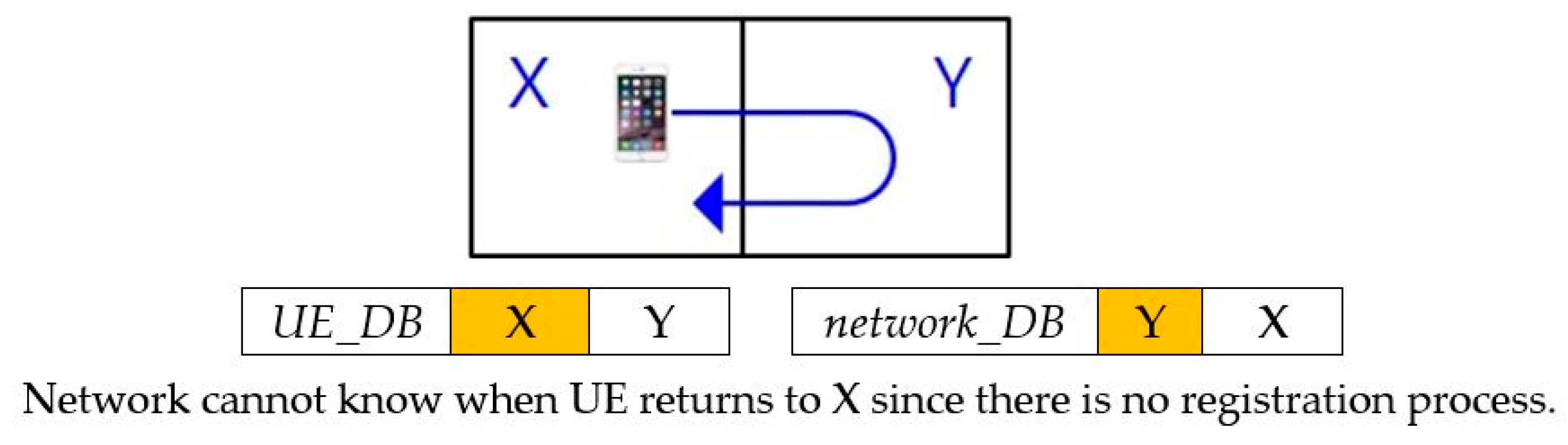
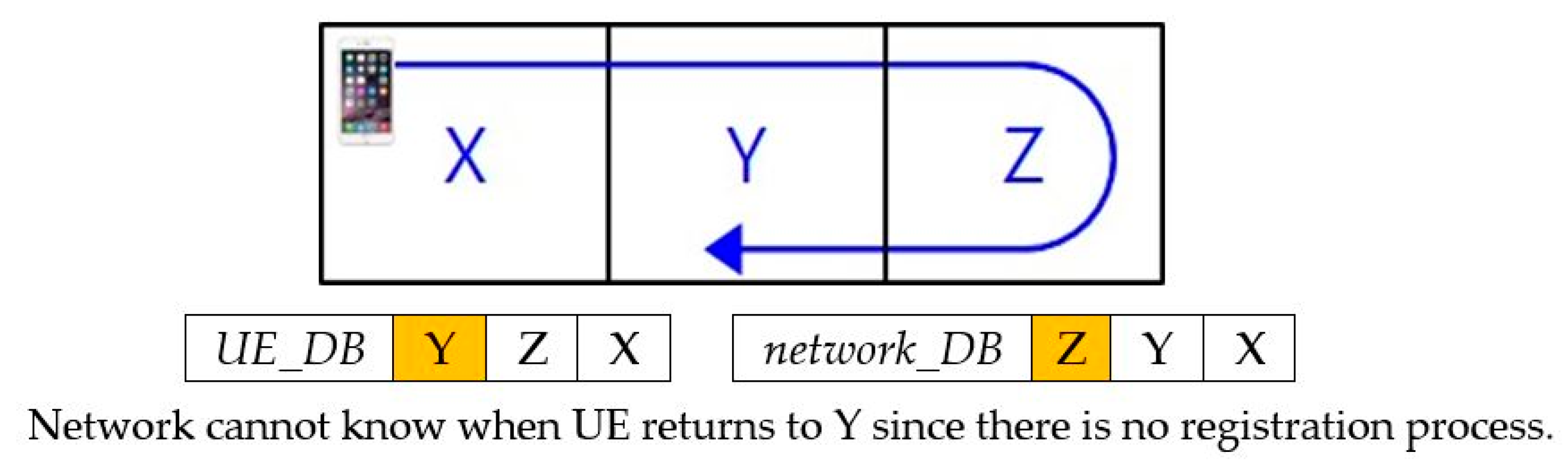
2. Zone-Based Registration

Let us consider zone-based registration with multiple zones. First, let us take a brief look at zone-based registration using two zones (2Z).

If UE uses two zones, as shown in Figure 1, location registration will not occur if the UE leaves and returns to zone X where it was initially registered. In this case, however, the network knows that the UE is in zone Y, where it was registered most recently. Therefore, the network starts paging zone Y first. If there is no response in this zone, it then pages zone X to receive an acknowledgement. As a result, location registration decreases, but paging load increases compared to zone-based registration with one zone (1Z). In order to obtain an accurate paging load, the probability of being in zone X, not the most recently registered zone, must be determined [1].

Let us now look at zone-based registration with three zones (3Z), which is the main subject of this study. If the UE uses three zones, as shown in Figure 2, location registration will not occur when the UE leaves and returns to zone Y where it had already been registered. On the other hand, the probability of returning to stored zones (X or Y) against staying in the most recently registered zone (Z) increases compared to a 2Z system, which increases paging load. As a result, location registration is reduced, but the paging load is increased compared to 1Z or 2Z systems.

In this study, a semi-Markov process model was developed to present an accurate mathematical model for a 3Z system.

3. New Mathematical Model

In this section, we propose a new mathematical model based on a semi-Markov process theory, to analyze the accurate performance of the 3Z system from the viewpoint of the total signaling cost on radio channels.

3.1. Notations and Assumptions

We define the following notations to analyze the signaling cost on radio channels.

▪

C_p: Signaling cost for paging per cell on radio channels

▪

C_u: Signaling cost for one location registration on radio channels

▪

θ: Probability of returning to the registered zone

▪

n: Number of cells per zone

▪

T_i: Interval between two incoming calls (r.v. (random variable), T_i ~Exp(1/λ_i), E(T_i) = 1/λ_i)

▪

T_o: Interval between two outgoing calls (r.v., T_o ~Exp(1/λ_o), E(T_o) = 1/λ_o)

▪

T_c: Interval between two calls (r.v., T_c ~Exp(1/λ), E(T_c) = 1/λ)

▪

T_m: Sojourn time in a zone (r.v., E(T_m) = 1/μ)

▪

R_m: Interval between the arrival of the call, and the time when the UE moves out of the zone (r.v.)

▪

ρ: Incoming calls to mobility ratio (CMR = λ_i/μ = ρ)

▪

$f_m^{\ast }\left(s\right)$: Laplace–Stieltjes transform for T_m (=${{\displaystyle \int }}_{t=0}^{\infty }{e}^{-st}{f}_m\left(t\right)dt)$

In addition, we assume the following for square zones, as shown in Figure 1 and Figure 2, in order to analyze the registration load over 3Zs.

▪

The interval between two calls, T_c, follows an exponential distribution with mean 1/λ.

▪

The UE’s sojourn time in a zone, T_m, follows a general distribution with mean 1/μ.

▪

The probability that UE returns to the last zone is θ.

▪

The probability that UE moves to one of the three zones except the last zone is the same (in other words, (1 − θ)/3).

▪

Call holding time is so short that it can be ignored.

Note that, by the additivity of Poisson processes [20], incoming calls with rate λ_i and outgoing calls with rate λ_o form a total call rate λ (= λ_i+ λ_o).

3.2. Semi-Markov Process Model for 3Z

Many studies on location registration assume that sojourn time in a zone follows an exponential distribution. On the other hand, our model applies to any general distributions for sojourn time in a zone only if its Laplace–Stieltjes transform can be obtained.

Furthermore, many studies employ a symmetric random-walk mobility model that gives the same probability of moving to any of the neighboring zones. However, it is easy to see that these assumptions are not realistic when considering the mobility of the actual UE. Normally, the next zone of the UE is related to the current zone. Therefore the assumption of a symmetric random walk is not realistic and does not reflect true UE behavior. Therefore, the probability of returning to the previous zone is assumed to be θ to reflect the dependency between the current zones and the next zone [1,10,11]. In a square zone environment, as shown in Figure 1 and Figure 2, θ would normally have a value greater than 0.25. Note that θ = 0.25 means a symmetric random walk model.

To illustrate the semi-Markov process model, we take into consideration the composition of the three zones for a 3Z system.

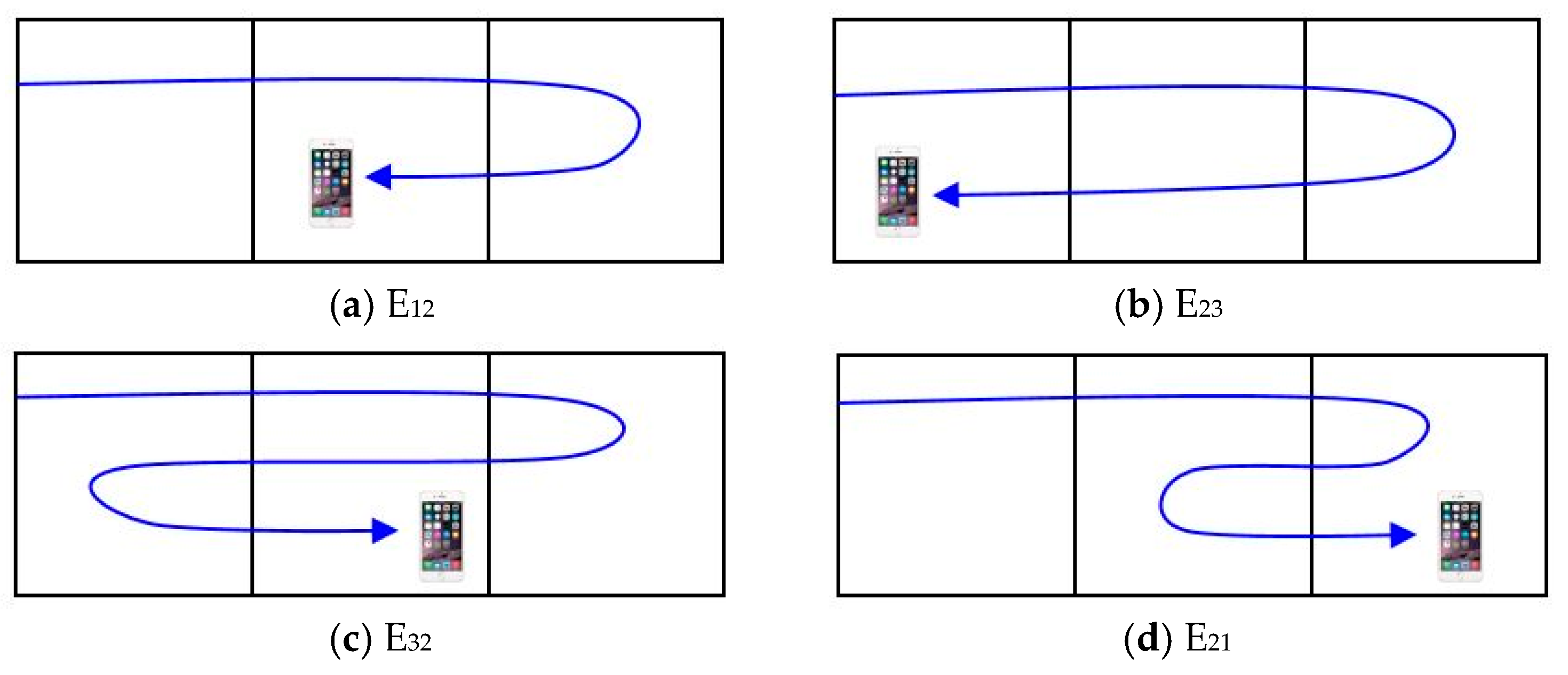
3.2.1. Definition of State by the Position of Each Zone in a 3Z System

Among the three zones, let us call the two zones at each end edge zones and the middle zone center zone and mark them as E and C, respectively. Sometimes, it is simpler to mark the two edge zones as ① and ③, and the center zone as ②. Note that the edge zone, marked as ① (E₁), is where location registration occurred more recently than the other edge zone (E₃).

For example, let us assume UE moves in the order of zone X (and registers) → zone Y (and registers) → zone Z (and registers) → zone Y, as shown in Figure 3. In this situation, zone X and zone Z are the edge zones, and zone Z is where location registration occurred most recently, we define this as state 1.

Let us define the state where we apply our semi-Markov process model. We define the following states with respect to the regular case.

E_ij (i = 1, 2, 3; j = 1, 2, 3)

C_ij (i = 1, 2, 3; j = 1, 2, 3)

E and C indicate that the most recently registered zones are an edge or center zones, respectively. The first subscript i (= 1, 2, 3) represents the UE’s immediately previous zone, the second subscript j (= 1, 2, 3) indicates the UE’s current zone.

For example, for the case of the UE shown in Figure 3, its state is E₁₂ since the current zone is the center (j = 2) and the last zone is the edge zone where it registered its location (i = 1). If the UE in Figure 3 returns to zone X, its state will be E₂₃ since the last zone is the center (i = 2) and the current zone is the edge zone where it did not register its location most recently (j = 3). In addition, if the above UE with a state of E₂₃ returns to zone Y, its state will be E₃₂ since the last zone is the edge zone where it did not register its location most recently (i = 3) and the current zone is the center (j = 2).

On the other hand, if the UE in Figure 3 returns to zone Z, its state will be E₂₁ since the last zone is the center (i = 2) and the current zone is the edge zone where it registered its location most recently (j = 1).

Figure 4 presents a collection of examples for states E_ij.

Example for C_ij (i = 1, 2, 3; j = 1, 2, 3) will be given in the next subsection for better understanding.

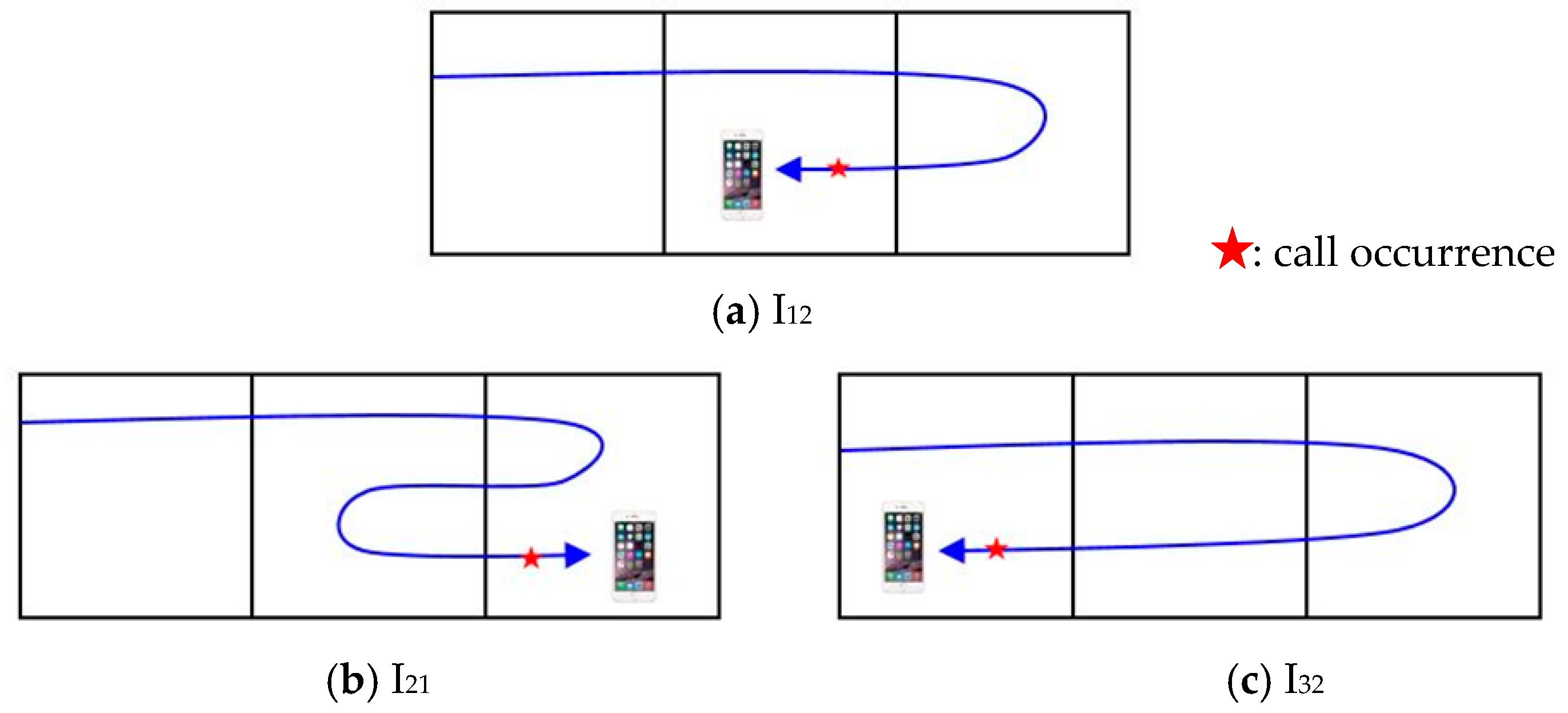
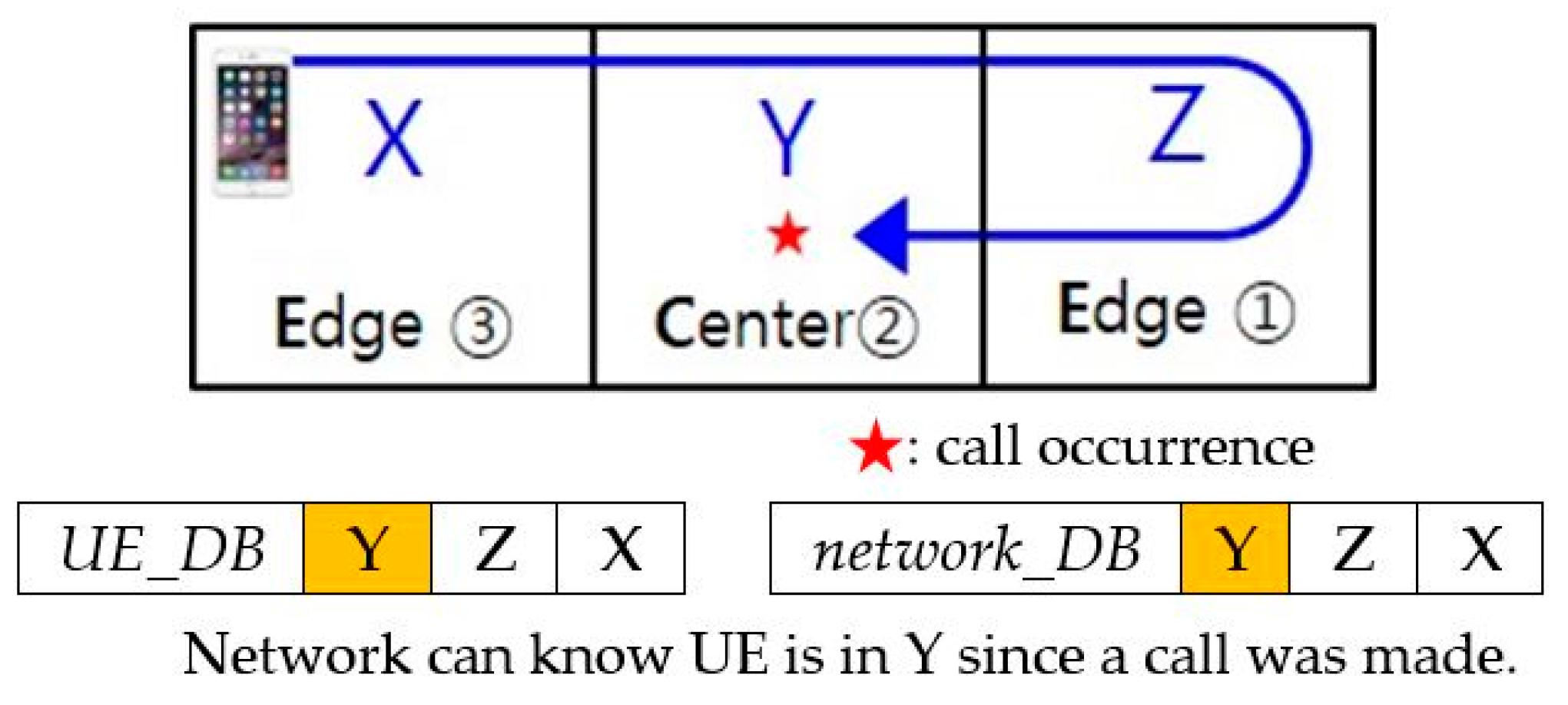
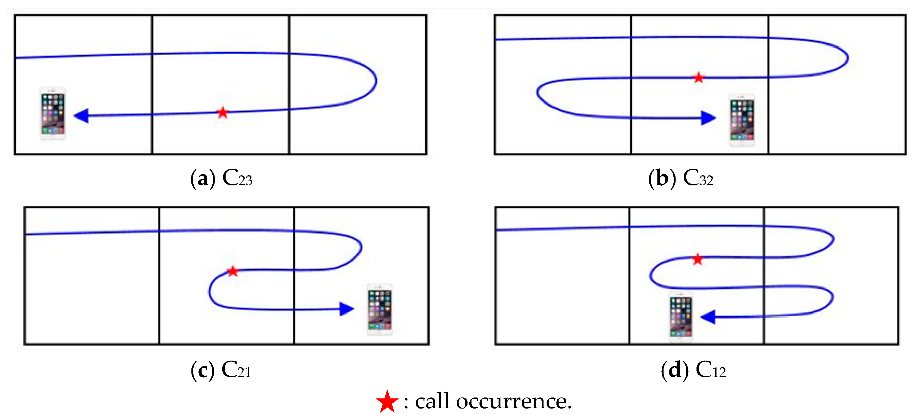
3.2.2. Definition of States by the Call Occurrence of Each Zone in a 3Z System

Location registration is divided into two main categories [9,10,11]. The first category is if the UE moves to a new zone that is not a previously stored zone, then it registers the location. The second category is if a call occurs from/to the UE in the current zone, the network updates the location. In the case of the first category, a location registration message is actually sent to the network. In the case of the second category, a separate location registration message is not delivered to the network, but the network can infer the UE’s zone through the call processing messages. The first category is referred to as regular registration (RR) and the second category is referred to as implicit registration (IR).

In the case of the first category, when the UE enters a new zone, the corresponding state is defined and the time it stays in that state is the total sojourn time in that zone. On the other hand, in the case of the second category, when a UE is currently in a zone and a call occurs from/to the UE, the corresponding state is defined so that the time it takes to stay in that state is typically less than the total sojourn time in that zone. In other words, we introduce state I to distinguish cases in the second category from cases in the first category since the time in each state is different.

We define the following states with respect to the second category:

I_ij (i = 1, 2, 3; j = 1, 2)

I indicates that UE receives/generates a call to register its location by IR. The first subscript i (= 1, 2, 3) represents the UE’s immediately previous zone, the second subscript j (= 1, 2) indicates the UE’s current zone.

It is sufficient to define only states I₂₁, I₁₂ and I₃₂ concerning call occurrence. For example, if UE with a state of E₂₁, E₁₂ and E₃₂ receives/generates a call, the UE’s zone remains the same but the states are changed to I₂₁, I₁₂ and I₃₂ respectively.

Figure 5 presents a collection of examples for states I_ij.

Note that if UE with a state of E₂₃ or C₂₃ receives/generates a call, its state will not be I₂₃ but I₂₁ since the last zone is the center (i = 2) and the current zone is the edge zone where it registered its location most recently (j = 1) by IR, which means that I₂₃ is not necessary.

For another example, let us say in the case of the UE shown in Figure 6, its state becomes I₁₂ when a call occurs since its state was E₁₂ just before the call occurred. If the UE returns to zone X, its state will be C₂₃ since the last zone is the center (i = 2) and the current zone is the edge zone where it did not register its location most recently (j = 3). In addition, if the above UE with a state of C₂₃ returns to zone Y, its state will be C₃₂ since the last zone is the edge zone where it did not register its location most recently (i = 3) and the current zone is the center (j = 2).

On the other hand, if the UE in Figure 6 returns to zone Z, its state will be C₂₁ since the last zone is the center (i = 2) and the current zone is the edge zone where it registered its location most recently (j = 1). In addition, if the above UE with a state of C₂₁ returns to zone Y, its state will be C₁₂ since the last zone is the edge zone where it registered its location most recently (i = 1) and the current zone is the center (j = 2).

Figure 7 presents a collection of examples for states C_ij.

3.2.3. Paging Procedure

In this study, it is assumed that sequential paging to the three zones was performed. When an incoming call occurred, the paging procedure was completed if there was a response from the paged zone. If there was no response, paging was performed again for the remaining zones.

The paging order should be determined to minimize paging costs. In this study, the most recently registered zone is paged first. If there is no response, the center zone is paged next. If there is no response again, the remaining edge zone is paged. Note that if the UE is in state I_ij, the first paging attempt always succeeds.

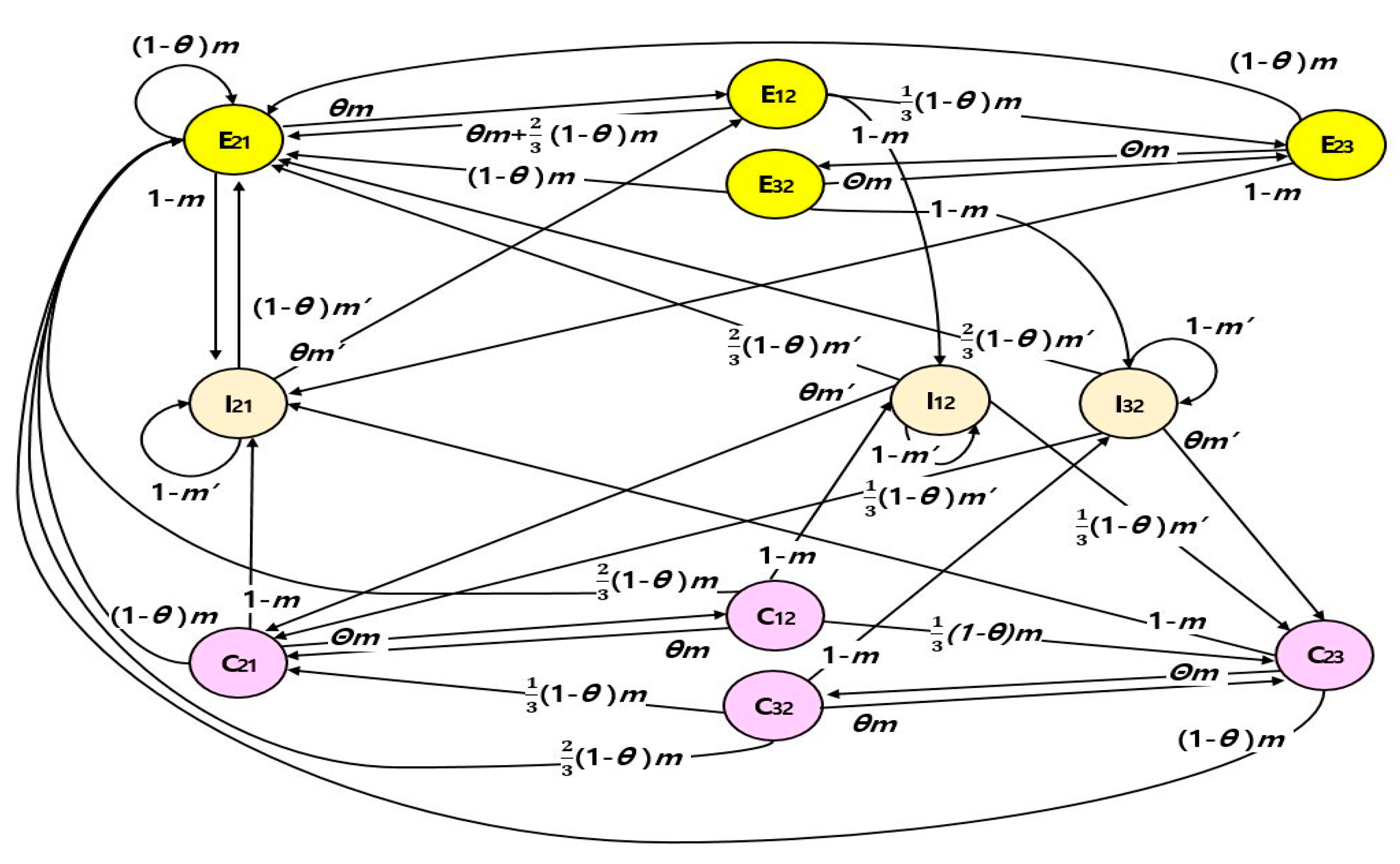
3.2.4. States for Semi-Markov Process and Transition Diagram

A summary of all the defined states is in

Table 1. States for the semi-Markov process model.

State	The Last Zone	Current Zone	Most Recently Registered Zone	No. of Paging
E21	2	1	edge (1)	1
E32	3	2	edge (1)	2
E12	1	2	edge (1)	2
E23	2	3	edge (1)	3
C21	2	1	center (2)	2
C12	1	2	center (2)	1
C32	3	2	center (2)	1
C23	2	3	center (2)	3
I21	2	1	edge (1)	1
I12	1	2	center (2)	1
I32	3	2	center (2)	1

.

The zone registered most recently by the UE can be the edge or center zone as shown in the table above. Additionally, all the states of the UE can be defined by classifying its state with respect to the last and current zones.

If the UE’s current zone is an edge zone, regardless of whether or not the edge zone is 1 or 3, the last zone is unconditionally a center zone. As a result, these states are expressed as E₂₁ or E₂₃. If the state is E₂₃, this means that the UE’s most recently registered location is in an edge zone and it moved to the other edge zone that is already in the zone list. If the status is E₂₁, this means that the UE’s most recently registered location is in an edge zone and it moved to another zone that is already in the zone list and its current zone is an edge zone in which it registered its location most recently.

Through a time-consuming process, a state transition diagram for all the states was obtained, as shown in Figure 8.

3.2.5. Calculation of State Transition Probabilities

Note that, in the state transition diagram, every transition probability contains m or m’. The first m is the probability that the UE is in a zone and will move to the neighboring zone before a call to/from the UE occurs. m can be obtained using the following equation:

$$m=P(T_c>T_m)={{\displaystyle \int }}_{t_m=0}^{\infty }{{\displaystyle \int }}_{t_c=t_m}^{\infty }\lambda e^{\lambda t_c}{f}_m\left(t_m\right)d{t}_{m}d{t}_c=f_m^{\ast }\left(\lambda \right)$$

(1)

where $f_m^{\ast }\left(s\right)$ is the Laplace–Stieltjes transform for $T_m$ (=${{\displaystyle \int }}_{t=0}^{\infty }{e}^{-st}{f}_m\left(t\right)dt)$.

Next, let us derive m’ = P(T_c > R_m), which is the probability that the UE, whose state changed due to a call without movement to a new zone, will move to the neighboring zone before another call from/to the UE occurs.

The density function of R_m, f_r(t) comes from the random observer property [1],

$$f_r\left(t\right)=\mu {{\displaystyle \int }}_{\tau =t}^{\infty }{f}_m\left(\tau \right)d\tau =\mu \left(1-F_m\left(t\right)\right)$$

(2)

The Laplace–Stieltjes transform for the distribution is as follows:

$$\begin{array}{ll}\hfill f_r^{\ast }\left(s\right)& ={{\displaystyle \int }}_{t=0}^{\infty }{e}^{-st}{f}_r\left(t\right)dt={{\displaystyle \int }}_{t=0}^{\infty }{e}^{-st}\mu \left(1-F_m\left(t\right)\right)dt=\frac{\mu }{s}-{{\displaystyle \int }}_{t=0}^{\infty }{e}^{-st}\mu F_m\left(t\right)dt \\ & =\frac{\mu }{s}+{\left[\frac{\mu }{s}{e}^{-st}\mu F_m\left(t\right)\right]}_{t=0}^{\infty }-\frac{\mu }{s}{{\displaystyle \int }}_{t=0}^{\infty }{e}^{-st}{f}_m\left(t\right)dt=\frac{\mu }{s}\left(1-f_m^{\ast }\left(\lambda \right)\right)\end{array}$$

(3)

Then, we have:

$$\begin{gathered} m^{\prime }=P(T_c>R_m)={{\displaystyle \int }}_{r_m}^{\infty }{{\displaystyle \int }}_{t_c=r_m}^{\infty }\lambda e^{-\lambda t_c}{f}_r\left(r_m\right)d{t}_{c}d{r}_m={{\displaystyle \int }}_{r_m=0}^{\infty }{f}_r\left(r_m\right)e^{-\lambda t_c}d{r}_m \\ =\frac{\mu }{\lambda }\left(1-f_m^{\ast }\left(\lambda \right)\right). \end{gathered}$$

(4)

3.2.6. Calculation of Sojourn Time in Each State

It is necessary to note that the sojourn time of state I_ij (i = 1, 2, 3; j = 1, 2, 3) is different from the sojourn time of state E_ij (i = 1, 2, 3; j = 1, 2, 3) or state C_ij (i = 1, 2, 3; j = 1, 2, 3). The sojourn time of state E_ij (i = 1, 2, 3; j = 1, 2, 3) or state C_ij (i = 1, 2, 3; j = 1, 2, 3) is the interval from the time a UE enters a zone until the time it leaves. On the other hand, the sojourn time of state I_ij (i = 1, 2, 3; j = 1, 2, 3) is the interval from the time a call to/from a UE occurs in a zone, until the time it leaves.

In the transition diagram, the UE in state E₂₁ (the state that the UE registered when moving from the center zone to an edge zone) can transit to one of three states: (i) If it moves to a new zone (with probability (1 – θ)P(T_c > T_m) = (1 – θ)m), its state becomes E₂₁ again. (ii) If it returns to the last zone (with probability θP(T_c > T_m) = θm), its state becomes E₁₂. (iii) If a call from/to the UE occurs before the UE moves to a neighboring zone (with probability P(T_c < T_m) = 1 – P(T_c > T_m) = 1 – m), UE’s state changes to state I₂₁.

We should consider the sojourn time of each state to be different, in order to derive an accurate probability of the first paging failure.

Now, let us derive the sojourn time of state I_ij (i = 1, 2, 3; j = 1, 2, 3). Since the sojourn time of state I_ij (i = 1, 2, 3; j = 1, 2, 3) can be expressed as:

$$T_I=\{\begin{array}{cc}{T}_c, & if T_c\le R_m\\ R_m,& if T_c>R_m\end{array}$$

and its mean can be derived as follows:

$$\begin{array}{ll}\hfill {\tau }_I& ={{\displaystyle \int }}_0^{\infty }{{\displaystyle \int }}_0^{r_m}{t}_c{f}_c\left(t_c\right)d{t}_c{f}_r\left(r_m\right)d{r}_m+{{\displaystyle \int }}_0^{\infty }{{\displaystyle \int }}_{r_m}^{\infty }{r}_m{f}_c\left(t_c\right)d{t}_c{f}_r\left(r_m\right)d{r}_m\\ & ={{\displaystyle \int }}_0^{\infty }[{{\displaystyle \int }}_0^{r_m}{t}_c{f}_c\left(t_c\right)d{t}_c+{{\displaystyle \int }}_{r_m}^{\infty }{r}_m{f}_c\left(t_c\right)d{t}_c]f_r\left(r_m\right)d{r}_m\\ & ={{\displaystyle \int }}_0^{\infty }[\frac{1}{\lambda }\left(1-e^{-\lambda r_m}\right)]f_r\left(r_m\right)d{r}_m=\frac{1}{\lambda }\left(1-f_r^{\ast }\left(\lambda \right)\right)\\ & =\frac{1}{\lambda }(1-\frac{\mu }{\lambda }\left[1-f_m^{\ast }\left(\lambda \right)\right])\end{array}$$

(5)

Next, let us derive the sojourn time of state E_ij (i = 1, 2, 3; j = 1, 2, 3) or state C_ij (i = 1, 2, 3; j = 1, 2, 3). Since the sojourn time of state E_ij (i = 1, 2, 3; j = 1, 2, 3) or state C_ij (i = 1, 2, 3; j = 1, 2, 3) can be expressed as:

$$T_E=\{\begin{array}{cc}{T}_c, & if T_c\le T_m \\ T_m,& if T_c>T_m\end{array}$$

and its mean can be derived as follows:

$$\begin{gathered} {\tau }_E={\tau }_C={{\displaystyle \int }}_0^{\infty }{{\displaystyle \int }}_0^{t_m}{t}_c{f}_c\left(t_c\right)d{t}_c{f}_m\left(t_m\right)d{t}_m+{{\displaystyle \int }}_0^{\infty }{{\displaystyle \int }}_{t_m}^{\infty }{t}_m{f}_c\left(t_c\right)d{t}_c{f}_m\left(t_m\right)d{t}_m= \\ {{\displaystyle \int }}_0^{\infty }[{{\displaystyle \int }}_0^{t_m}{t}_c{f}_c\left(t_c\right)d{t}_c+{{\displaystyle \int }}_{t_m}^{\infty }{t}_m{f}_c\left(t_c\right)d{t}_c]f_m\left(t_m\right)d{t}_m={{\displaystyle \int }}_0^{\infty }[\frac{1}{\lambda }\left(1-e^{-\lambda t_m}\right)]f_m\left(t_m\right)d{t}_m= \\ \frac{1}{\lambda }\left(1-f_m^{\ast }\left(\lambda \right)\right) \end{gathered}$$

(6)

3.2.7. Calculation of Steady-State Probabilities

To get the steady-state probability $\tilde{\pi }$ considering the different sojourn times, we first calculate the steady-state probability π for the usual Markov chain with transition probability P. This can be obtained by using the following balanced equations [20]:

$$\mathit{\pi }\mathit{P}=\mathit{\pi }, {{\displaystyle \sum }}_i{{\displaystyle \sum }}_j({\pi }_{Cij}+{\pi }_{Eij}+{\pi }_{Iij})=1$$

(7)

Then, the final steady-state probability of the semi-Markov process can be obtained as below [6]:

$$\begin{gathered} {\tilde{\pi }}_{Cij}=\frac{{\pi }_{Cij}{\tau }_C}{{{\displaystyle \sum }}_i{{\displaystyle \sum }}_j({\pi }_{Cij}{\tau }_C+{\pi }_{Eij}{\tau }_E+{\pi }_{Iij}{\tau }_I)} \\ {\tilde{\pi }}_{Eij}=\frac{{\pi }_{Eij}{\tau }_E}{{{\displaystyle \sum }}_i{{\displaystyle \sum }}_j({\pi }_{Cij}{\tau }_C+{\pi }_{Eij}{\tau }_E+{\pi }_{Iij}{\tau }_I) } \\ {\tilde{\pi }}_{Iij}=\frac{{\pi }_{Iij}{\tau }_I}{{{\displaystyle \sum }}_i{{\displaystyle \sum }}_j({\pi }_{Cij}{\tau }_C+{\pi }_{Eij}{\tau }_E+{\pi }_{Iij}{\tau }_I)} \end{gathered}$$

(8)

3.3. Registration Cost

By making the assumption that U is the registration cost of one registration, the registration cost between two incoming calls, Cu, can be obtained as follows:

$$\begin{array}{ll}\hfill C_U& =U·\frac{\mu }{{\lambda }_i}·[{\tilde{\pi }}_{I21}\left(1-\theta \right)m^{\prime }+\left({\tilde{\pi }}_{I32}+{\tilde{\pi }}_{I12}\right)\frac{2}{3}\left(1-\theta \right)m^{\prime }\\ & +\left({\tilde{\pi }}_{E21}+{\tilde{\pi }}_{C21}+{\tilde{\pi }}_{E23}+{\tilde{\pi }}_{C23}\right)\left(1-\theta \right)m\\ & +\left({\tilde{\pi }}_{E12}+{\tilde{\pi }}_{E32}+{\tilde{\pi }}_{C12}+{\tilde{\pi }}_{C32}\right)\frac{2}{3}\left(1-\theta \right)m]\end{array}$$

(9)

3.4. Paging Cost

As described in Section 3.2, it is assumed that three-step sequential paging to the three zones was performed. The most recently registered zone is paged first. If there is no response, the center zone is paged next. If there is no response again, the remaining edge zone is paged.

Let us consider the paging cost of a 3Z system when the above three-step sequential paging is applied. Assuming V to be the paging cost for one cell, the paging cost between two incoming calls, C_P, can be obtained as follows:

$$\begin{array}{ll}\hfill C_P& =V·(n·P[1\mathrm{st}\mathrm{paging}\mathrm{success}]+2n·P\left[2\mathrm{nd}\mathrm{paging}\mathrm{success}\right]+3·P\left[3\mathrm{rd}\mathrm{paging}\mathrm{success}\right])\\ & =V·[n\left({\tilde{\pi }}_{E21}+{\tilde{\pi }}_{I21}+{\tilde{\pi }}_{I32}+{\tilde{\pi }}_{I12}+{\tilde{\pi }}_{C12}+{\tilde{\pi }}_{C32}\right)+2n\left({\tilde{\pi }}_{E12}+{\tilde{\pi }}_{E32}+{\tilde{\pi }}_{C21}\right)\\ & +3n\left({\tilde{\pi }}_{E23}+{\tilde{\pi }}_{C23}\right)]\\ & =V·\left[2n-n·\left({\tilde{\pi }}_{E21}+{\tilde{\pi }}_{C21}+{\tilde{\pi }}_{I21}+{\tilde{\pi }}_{I32}+{\tilde{\pi }}_{I12}\right)+n·\left({\tilde{\pi }}_{E23}+{\tilde{\pi }}_{C23}\right)\right]\end{array}$$

(10)

3.5. Total Cost

As a result, the final total cost between two incoming calls can be obtained by adding the paging cost to the registration cost.

$$T{C}_{3Z}=C_U+C_P$$

(11)

4. Numerical Results

We obtained numerical results for 1Z, 2Z and 3Z systems and compared their performances. We assumed the following:

▪

The number of cells in a zone, n, is 4.

▪

The probability of returning to the last zone, θ, is 0.4.

▪

Registration cost of one registration, U, is 4 and paging cost for one cell, V, is 1 (U = 4, V = 1).

▪

Incoming and outgoing call rates are both 1 call per hour (λ_i = λ_o = 1).

▪

UE’s sojourn time in a zone, T_m, follows an exponential distribution with mean 1/4 (μ = 4).

The probability of returning to the last zone, θ, is chosen arbitrarily so that it is larger than 0.25 (symmetric random walk) referring to other research results [1,9,10,11,12].

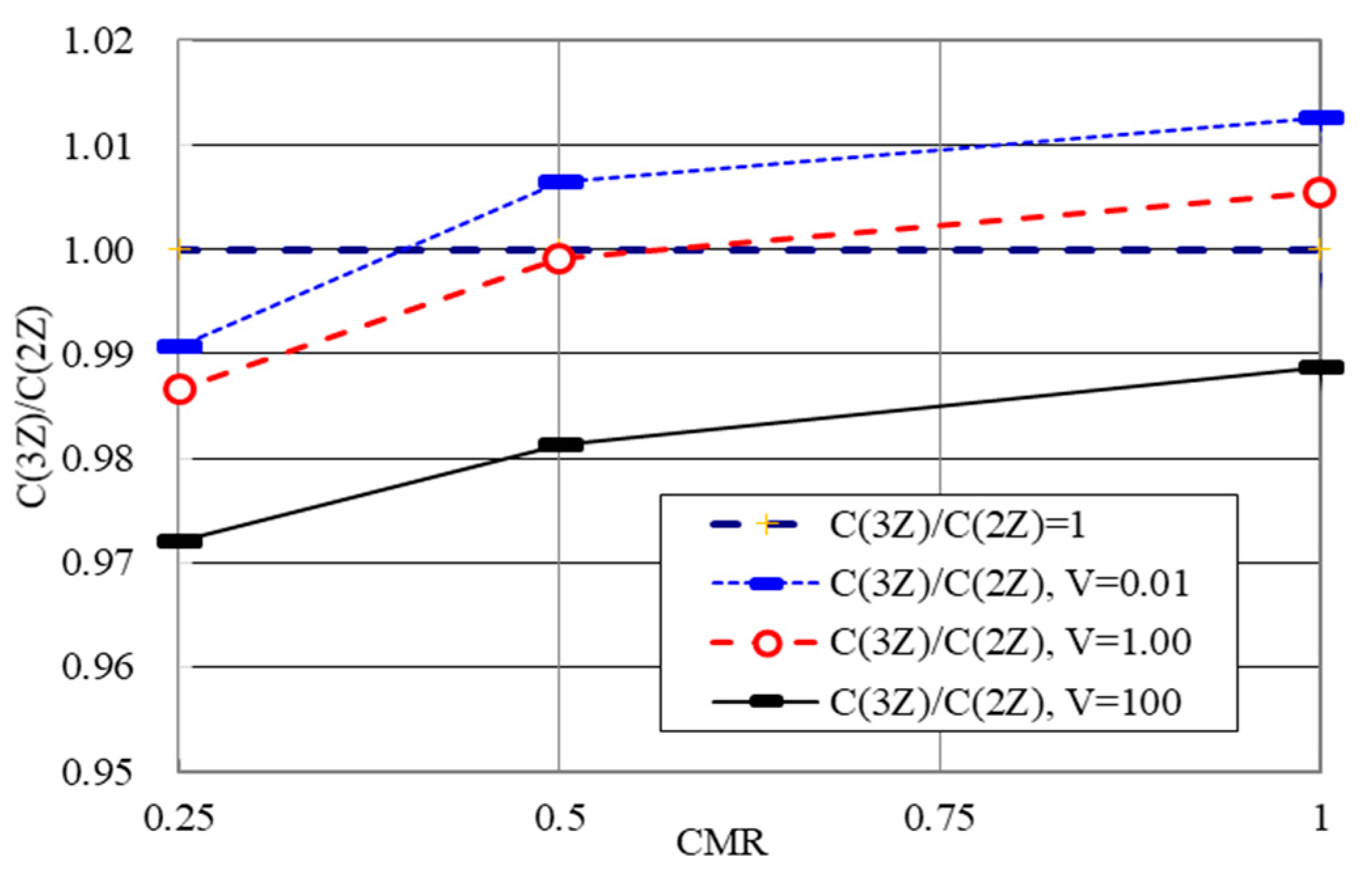
4.1. Total Cost for Various CMRs

Figure 9 shows the total costs of 1Z, 2Z and 3Z systems for various call-to-mobility (CMR = λ_i/μ) ratios. CMR = 1/2 indicates that the UE entered two zones between incoming calls. Note that a smaller CMR means that the UE entered more zones between incoming calls. The CMR value is considered from 0.125 to 1.00 to consider real situations. From the figure, we can see that 3ZR outperforms not only 1Z but also 2Z. We can also see that, as CMR decreases, the relative gap between 1Z/2Z and 3Z increases. Even if 3Z is expected not to outperform 1Z/2Z especially when CMR is very high, such a high CMR seems to be unrealistic. In summary, 3ZR generally outperforms 1Z and 2Z in real situations.

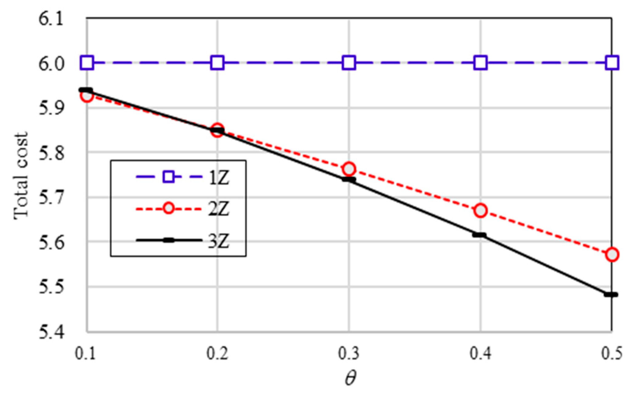
4.2. Total Cost for Various Probabilities of Moving Back to the Last Zone

Figure 10 shows the total cost for various probabilities of moving back to the last zone, θ, when CMR = 1 and n = 4. The total cost of 2Z and 3Z systems decrease as θ increases but the total cost of the 3Z system decreases more than that of a 2Z system in our environment, as clearly shown in Figure 10. From the figure, we can see that, noting that θ is generally greater than or equal to 0.25 in a square zone environment, 3Zs are optimal in most cases.

4.3. Total Cost for Various Gamma Distributions

Let us consider the case where the UE’s sojourn time in a zone, T_m, follows a gamma distribution with a mean of 1 and focus on the comparison between 2Z and 3Z systems since they are both far superior to a 1Z system.

Assuming θ = 0.3, Figure 11 compares the performance results for various CMRs and variances. The figure shows that the 3Z system is superior to the 2Z system for small CMRs. We can also see that, as the variance decreases, this tendency becomes more definite. Note that, from the figure, the smaller the CMR and the larger the variance, the better the 3Z system is compared to the 2Z system but the difference is very small (about 1%).

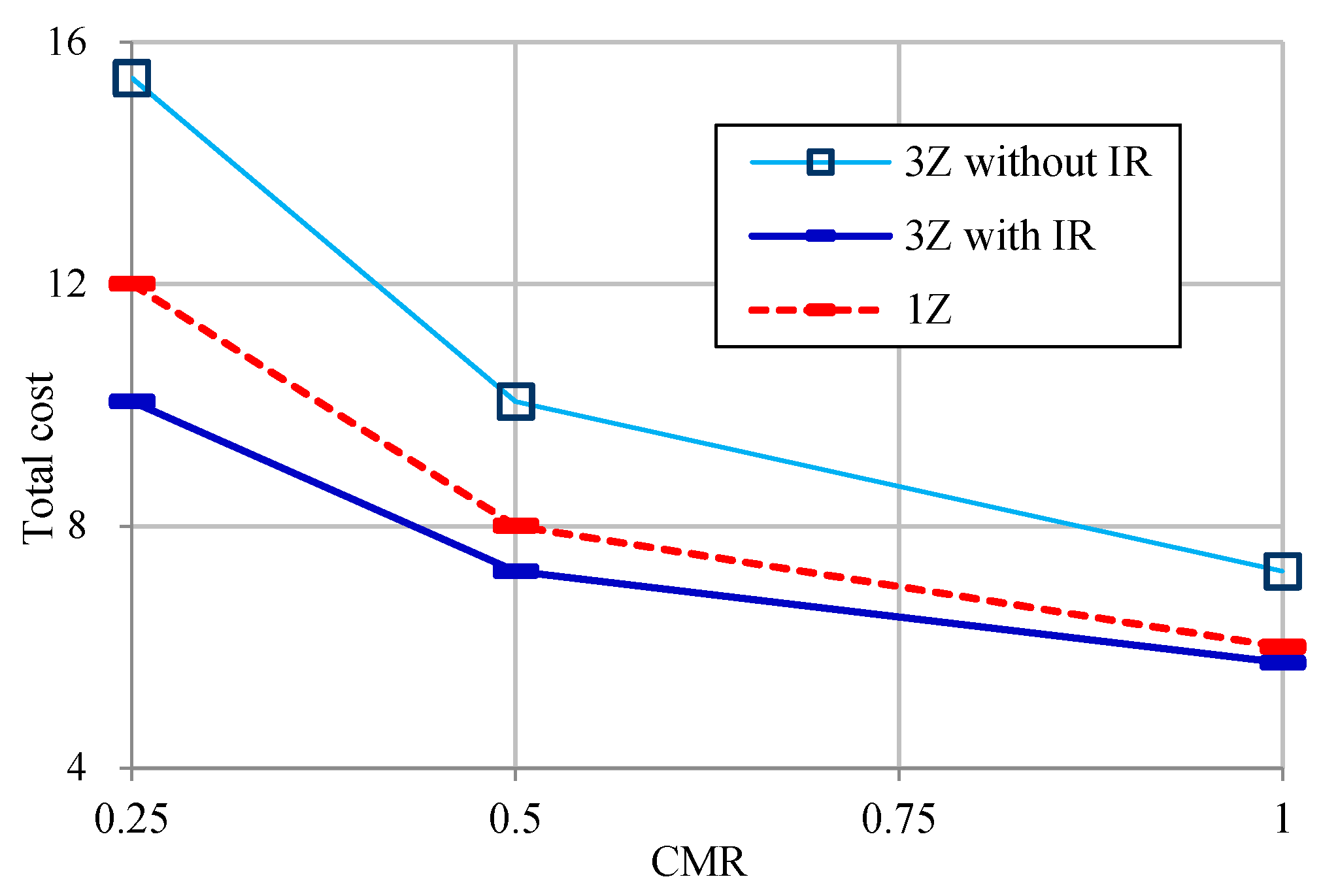
4.4. Effect of Implicit Registration by Outgoing Calls

As explained in Section 3, when a call is made from the UE in the current zone, the network updates the location through the call processing messages without location registration messages, which is called an implicit registration (IR) by an outgoing call. In this case, the paging cost can be reduced in 2Z or 3Z systems since the network can infer the UE’s current zone.

Let us examine the IR effect by outgoing calls in a 3Z system numerically. Figure 12 compares the performance results for a 3Z system without IR, a 3Z system with IR and a 1Z system for some CMRs, while assuming T_m follows an exponential distribution with a mean of 1. In this case, it is also assumed that the outgoing call rate is equal to the incoming call rate (${\lambda }_i={\lambda }_o$). In the figure, we can see that the 3Z system with IR is much superior to a 3Z system without IR. Note that when IR is not considered, the 3Z system is inferior to the 1Z system but when IR is considered, the 3Z is superior to the 1Z system. In conclusion, the IR effect by outgoing calls should be considered for the 3Z system to achieve a minimal total cost.

4.5. Effects of the Number of Cells in a Zone and the Registration Cost of One Registration

In this section, the number of cells in a zone, n, is assumed to be 4. The number of cells in a zone (n) directly affects the paging cost C_P. As n increases, C_P increases proportionally. From the viewpoint of 3Z, the increase of n may degrade the performance of 3Z since the paging cost C_P increases steeply compared to 1Z or 2Z. As a result, if n is far greater than 4, 3Z may show worse performance than 2Z. On the other hand, if n is far less than 4, 3Z may show better performance than 2Z.

Note that this kind of scalability can be applied to the other parameters in the similar way. For example, let us consider registration cost. In this section, the registration cost of one registration, U, is assumed to be 4. U directly affects the registration cost C_U. As U increases, C_U increases proportionally. From the viewpoint of 3Z, the increase of U may upgrade the performance of 3Z since the location registration cost C_U increases moderately compared to 1Z or 2Z. As a result, if U is far greater than 4, 3Z may show better performance than 2Z. On the other hand, if U is far less than 4, 3Z may show worse performance than 2Z.

5. Conclusions

In this study, we proposed a very simple new mathematical model using semi-Markov process theory for zone-based registration using three zones (3Z) and analyzed the performance of a 3Z system using the proposed model. The numerical results for the various situations showed that, when the CMR is small, the 3Z system outperforms 1Z and 2Z systems. On the other hand, when the CMR is very large, the 3Z is not much different from 1Z or 2Z systems or is sometimes inferior to 1Z and 2Z systems. In conclusion, depending on the system situation, the optimal management scheme for zone-based registration will change dynamically, so it is necessary to operate zone-based registration flexibly by considering the system situation.

Using a simple mathematical model based on semi-Markov process theory, this study can easily support the prompt determination of the optimal management scheme for zone-based registration. These results are directly able to enhance the performance of actual mobile networks and can be implemented quickly and easily. Since no hardware modifications are necessary to implement a 3Z system, it can be easily applied by modifying the 4G/5G networks of the existing 1Z based networks. Noting that a 3Z system outperforms a 2Z system in specific conditions, it is possible to adopt an adaptive scheme to dynamically switch between 1Z, 2Z or 3Z systems according to the current situation.

References

1. Lin, Y.B. Reducing location update cost in a PCS network. IEEE/ACM Trans. Netw. 1997, 5, 25–33. [Google Scholar]
2. 3GPP2 C.S0005-E Version 3.0, Upper Layer (Layer 3) Signaling Standard for cdma2000 Spread Spectrum Systems. June 2011. Available online: http://www.3gpp2.org/Public_html/Specs/C.S0005-E_v3.0_cdma2000_1x_Layer-3_20110620.pdf (accessed on 17 August 2020).
3. Li, J.; Kameda, H.; Li, K. Optimal dynamic mobility management for PCS networks. IEEE/ACM Trans. Netw. 2000, 8, 319–327. [Google Scholar]
4. Wang, X.; Lei, X.; Fan, P.; Hu, R.; Horng, S. Cost analysis of movement-based location management in PCS networks: An embedded Markov chain approach. IEEE Trans. Veh. Technol. 2014, 63, 1886–1902. [Google Scholar] [CrossRef]
5. Mao, Z.; Douligeris, C. A location-based mobility tracking scheme for PCS networks. Comput. Commun. 2000, 23, 1729–1739. [Google Scholar] [CrossRef]
6. Baek, J.H.; Lee, T.H.; Kim, J.S. Performance analysis of 2-location distance-based registration in mobile communication networks. IEICE Trans. Commun. 2013, E96-B, 914–917. [Google Scholar] [CrossRef]
7. Seo, K.H.; Baek, J.H.; Eom, C.S.; Lee, W. Optimal management of distance-based location registration using embedded Markov chain. Int. J. Distrib. Sens. Netw. 2020, 16. [Google Scholar] [CrossRef] [Green Version]
8. Baek, J.H.; Ryu, B.H.; Lim, S.K.; Kim, K.S. Mobility model and performance analysis for zone-based registration in CDMA mobile communication system. Telecommun. Syst. 2000, 14, 13–30. [Google Scholar] [CrossRef]
9. Jang, H.S.; Hwang, H.; Jun, K.P. Modeling and analysis of two-location algorithm with implicit registration in CDMA personal communication network. Comput. Ind. Eng. 2001, 41, 95–108. [Google Scholar] [CrossRef]
10. Baek, W.M.; Yoon, J.H.; Kim, C.S. Modeling and analysis of mobility management in mobile communication networks. Sci. World J. 2014, 2014, 250981. [Google Scholar] [CrossRef] [PubMed] [Green Version]
11. Baek, J.H. Analyzing zone-based registration in mobile cellular networks. IEICE Trans. Commun. 2017, E100-B, 2070–2078. [Google Scholar] [CrossRef]
12. Jung, J.; Baek, J.H. Modeling and cost analysis of zone-based registration in mobile cellular networks. ETRI J. 2018, 40, 736–744. [Google Scholar] [CrossRef]
13. Liou, R.H.; Lin, Y.B. Mobility management with the central-based location area policy. Comput. Netw. 2013, 57, 847–857. [Google Scholar] [CrossRef] [Green Version]
14. Lin, Y.B.; Liou, R.H.; Chang, C.T. A dynamic paging scheme for long-term evolution mobility management. Wirel. Commun. Mob. Comput. 2015, 15, 629–638. [Google Scholar] [CrossRef]
15. Deng, T.; Wang, X.; Fan, P.; Li, K. Modeling and performance analysis of a tracking-area-list-based location management scheme in LTE networks. IEEE Trans. Veh. Technol. 2016, 65, 6417–6431. [Google Scholar] [CrossRef]
16. Jung, J.; Baek, J.H. Reducing paging cost of tracking area list-based mobility management in LTE network. J. Supercomput. 2018. [Google Scholar] [CrossRef]
17. Alsaeedy, A.A.R.; Chong, E.K.P. Tracking area update and paging in 5G networks: A survey of problems and solutions. Mob. Netw. Appl. 2019, 24, 578–595. [Google Scholar] [CrossRef]
18. Chen, L.; Liu, H.L.; Fan, Z.; Xie, S.; Goodman, E.D. Modeling the tracking area planning problem using an evolutionary multi-objective algorithm. IEEE Comput. Intell. Mag. 2017, 12, 29–41. [Google Scholar] [CrossRef]
19. Alsaeedy, A.A.R.; Chong, E.K.P. Mobility management for 5G IoT devices: Improving power consumption with lightweight signaling overhead. IEEE Internet Things J. 2019, 6, 8237–8247. [Google Scholar] [CrossRef]
20. Ross, S. Introduction to Probability Models, 11th ed.; Elsevier: Cambridge, MA, USA, 2014. [Google Scholar]
Figure 1. Zone-based registration with two zones.
Applsci 10 05705 g001
Figure 2. Zone-based registration with three zones.
Applsci 10 05705 g002
Figure 3. Edge and center zones in a 3Z system.
Applsci 10 05705 g003
Figure 4. Examples of states Eij.: (a) E12; (b) E23; (c) E32; (d) E21.
Applsci 10 05705 g004
Figure 5. Examples of states Iij.: (a) I12; (b) I21; (c) I32.
Applsci 10 05705 g005
Figure 6. A call occurs in a 3Z system.
Applsci 10 05705 g006
Figure 7. Examples of states Cij.: (a) C23; (b) C32; (c) C21; (d) C12.
Applsci 10 05705 g007
Figure 8. State transition diagram for a 3Z system.
Applsci 10 05705 g008
Figure 9. Total cost for various CMR.
Applsci 10 05705 g009
Figure 10. Total cost for various θs.
Applsci 10 05705 g010
Figure 11. Total cost for various gamma distributions (θ = 0.3).
Applsci 10 05705 g011
Figure 12. Effect of implicit registration by outgoing calls (θ = 0.3).
Applsci 10 05705 g012