Valve Internal Leakage Rate Quantification Based on Factor Analysis and Wavelet-BP Neural Network Using Acoustic Emission

Abstract

Valve internal leakage is easily found because of various defects resulting from environmental factors and load fluctuation. The timely detection of valve internal leakage is of great significance to the safe operation of pipelines. As an effective means for detecting valve internal leakage, the acoustic emission technique is characterized by nonintrusive and strong anti-interference ability, which can realize the in situ monitoring of the valve running status in real time. In this paper, acoustic emission signals from an internal leaking valve were obtained experimentally. Then, the dimensionality reduction technology based on factor analysis was introduced to the processing of valve internal leakage detection data. Next, the wavelet decomposition was carried out to decompose the sample feature set into four subsets. Finally, the decomposed sample feature sets were inputted into the error backpropagation (BP) neural network quantitative model, respectively. The optimized results show that the predicted internal leakage rate by the wavelet-BP neural network model has good precision with an error of less than 10%. The wavelet-BP neural network model can realize the analysis of the valve internal leakage rate quantitatively and has good robustness, which provides technical support and guarantees the safe operation of natural gas pipeline valves.

1. Introduction

In recent years, with the increasing use of natural gas, the pipe diameter and pressure of natural gas transmission pipelines have been increasing synchronously [1]. As a result, the valve size has also increased. The role of valves plays in ensuring the safe operation of pipelines is becoming more relevant. At the same time, the requirements for safety and reliability of valves are also increasing.

In the operation of natural gas pipeline valves, defects such as pitting corrosion, surface damage and overall fracture may occur, which may result in internal leakage [2,3]. If the internal leakage in a valve cannot be detected in time, it may cause the combustible gas to be pumped into the low-pressure manifold from the high-pressure pipe, which will bring serious safety hazards to the normal operation of the long-distance gas pipelines. Therefore, the timely and effective detection of the internal leakage in a valve is of great significance to ensure the safe operation of the pipelines.

Several kinds of techniques, including acoustic emission (AE) [4], vibration monitoring [5,6] and cavity dynamic pressure [7], have been used for the detection of valve internal leakage. Among these techniques, AE has witnessed a wide application in the detection of valve internal leakage both qualitatively and quantitatively, because it possesses the advantage of nonintrusive, high sensitivity and strong anti-interference ability [8,9,10]. As the accurate prediction of internal leakage is the basis for maintenance strategy, many scholars have been carrying out research on the quantitative evaluation of the valve internal leakage rate. In [11], an equation was established to relate the detected AE signal to the leakage rate at different valve-inlet pressures and valve sizes. In [12,13], AE signal power computed from the power spectral density correlated well with influenced factors of leakage rates, and a novel and inexpensive AE instrument was invented for predicting qualitative leakage rate using a microprocessor and derived relationship. In [14], correlation coefficients and the frequency spectra of the AE signals obtained were used to predict the leakage rate under certain conditions. In [15], a neural-network-based correlation model that detected the position of internal leakages successfully and quantified the number of rates within an acceptable error bound was proposed. In [16], the nonlinear regression method, kernel partial least-squares regression (KPLSR), with the distance kernel, was used for leakage rate quantification. In [17], the relationship between the standard deviation and the leakage rate was fitted by the least-squares method to establish the mathematical model of valve internal leakage. In [18], a model based on k-medoids clustering was used to recognize internal valve leakage rates. In [19], a regression-based deep belief network (DBN) was proposed to predict the internal leakage rates of a valve in a natural gas pipeline. In [20], The k-nearest neighbors and support vector machine classification algorithms were employed to classify the valve conditions before the estimation of the valve flow rate through the regression model. In [21], the Gaussian process regression was used to establish a multivariate mathematical model for describing the relationship between the characteristics of the AE signal and leakage rate. A comparison of the prediction methods above is shown in

Table 1. Comparison of different prediction methods for the valve internal leakage rate.

References	Methods	Error
[11]	Equation fitting	Between 9.2% and 29.7%
[12,13]	Power spectral density	Approximately ±7.8% full scale
[14]	Spectrum of frequencies	Not mentioned
[15]	Neural-network-based correlation model	≤1%
[16]	Nonlinear regression method, kernel partial least-squares regression	≤27%
[17]	Least-squares method	Not given
[18]	K-medoids clustering	Overall accuracy 96.28%
[19]	Regression-based deep belief network	≤20%
[20]	Regression method	Accuracy between 74.5% and 98.8%
[21]	Gaussian process regression	Not given

.

In this paper, a novel prediction method for the internal leakage rate of natural gas pipeline valves based on factor analysis and wavelet-BP neural network is proposed. Firstly, the factor analysis is introduced to realize the dimensionality reduction of acoustic emission signals of a valve. Then, the wavelet decomposition is used to decompose the sample feature set. Finally, the error backpropagation (BP) neural network model is established to predict the internal leakage rate of a valve quantitatively. The outline of the paper is as follows. The paper first introduces the theory and related algorithm in Section 2. Then, the acoustic emission experimental platform for detecting leakage in a valve is presented in Section 3. Section 4 presents and discusses the quantitative model of internal leakage and its prediction results. Finally, conclusions are made in Section 5.

2. Theory

2.1. Basic Theory of Acoustic Emission for Valve Detection

Acoustic emission is a phenomenon of transient elastic waves generated by materials or components accompanying energy release [22]. This kind of signal is collected by AE transducers, and the collected signals are analyzed to explore the problems of materials or components.

Valve internal leakage detection is an important application of acoustic emission technology. During the internal leakage of a valve, the fluid is jetted downstream through the leak hole under the action of the valve pressure to produce jet noise, which contains internal leakage information (including location of the internal leakage point, internal leakage flow rate) and interact with the valve wall to spread around [23]. The jet noise can be detected by a highly sensitive acoustic emission sensor. As a result, valve internal leakage can be identified qualitatively and quantitatively.

2.2. Data Dimensionality Reduction Based on Factor Analysis

The acoustic emission data of a valve contains a large number of high-dimensional features. These high-dimensional features bring many problems to the establishment of the quantitative model of the valve leakage rate. For example, the high-dimensional feature set contains a lot of redundant features, which increases the complexity of the model algorithm greatly, and increases the time and space complexity of the algorithm. Therefore, data dimensionality reduction technology has been introduced into high-dimensional data processing, aiming at reflecting most of the information of the original data with low-dimensional independent samples.

The factor analysis method is a kind of data dimensionality reduction method. Its core is to use a few sample sets to express almost all the information of high-dimensional data. Here the R-type factor analysis model is used. Let X = (X₁, X₂, …, X_p) be the raw sample data, F = (F₁, F₂, …, F_m) is an unknown vector. The raw sample data can be described as:

X_i = μ_i + α_i1F₁ + ⋯ + α_imF_m + ε_i,

(1)

Equation (1) can be expressed as matrix variance:

X − μ = AF + ε,

(2)

where F = (F₁, F₂, …, F_m) is the common factor of original sample data, the coefficients of which are factor loads. ε = (ε₁, ε₂, …, ε_m) is the special factor, the part that cannot be contained by the m common factors. F_i is the ith common factor of the original sample data. α_ij is the factor load. F_i is independent with each other, and their variance is 1.

2.3. Wavelet Decomposition

Wavelet decomposition refers to the decomposition of a sample into a high-frequency part and low-frequency part. Each layer of wavelet decomposition decomposes the sample into high-frequency and low-frequency parts. The wavelet decomposition process is shown in Figure 1. After the first layer wavelet decomposition of the sample, high-frequency D1 and low-frequency A1 are obtained. Next, in each layer decomposition, the low-frequency sample obtained from the previous layer is decomposed into two parts, high-frequency Dn and low-frequency An. Dn is the high-frequency signal decomposed by the nth layer, while An is the low-frequency signal decomposed by the nth layer.

In this study, wavelet decomposition will be performed on the sample feature set after dimensionality reduction by factor analysis. A three-layer wavelet decomposition will be performed on the sample feature set after dimensionality reduction to obtain four decomposed sample feature subsets.

2.4. BP Neural Network

As a neural network model using a multilayer perceptron, BP neural network is composed of the input layer, middle layer and output layer. Among them, the middle layer is the hidden layer, which can be a one-layer or multilayer structure. Figure 2 shows the structure of the BP neural network using the Sigmoid function as the activation function for both the hidden and output nodes.

In Figure 2, the input vector X = (x₁, x₂, …, x_n) is transferred to the first hidden layer, and the output vector A₁ = (a₁⁽¹⁾, a₂⁽¹⁾, …, a_n⁽¹⁾) is obtained by activation function. Then, A₁ is transferred to the second hidden layer, resulting in the output A₂ = (a₁⁽²⁾, a₂⁽²⁾, …, a_n⁽²⁾). Similarly, A₂ is transferred to the output layer, resulting in the output vector Y = (y₁, y₂, …, y_n). As a result, the prediction values and total loss function are obtained. Next, calculate the gradient of the weight matrix and bias vector of the loss function in each layer by the chain rule, which is the backpropagation of errors. In the end, update the weight matrix and bias vector of each layer by gradient descent method. Repeat the iteration until the loss function satisfies the requirement.

As described above, the computational procedure of the BP neural network consists of two periods, the forward propagation and the backpropagation. The learning steps of the BP neural network algorithm are as follows:

Step 1: Input the sample training set X = (x₁, x₂, …, x_n).

Step 2: Initialize the weight matrix and the bias vector.

Step 3: Calculate the output of each layer A₁, A₂, ⋯. For each layer, the output can be calculated by Equation (3):

a^(l) = f(W^(l)a^(l−1) + b^(l)),

(3)

where f = (.) is the activation function, W^(l) is the weight matrix of the lth layer, a^(l−1) is the output of the nerve cell in the (l − 1)th layer, b^(l) is the bias vector of the lth layer.

Step 4: Calculate the loss function by Equation (4):

$$J_{MSE}(W,b)=\frac{1}{2m}{\displaystyle \sum _{i=1}^m{\left[f(x^i)-y^i\right]}^2},$$

(4)

where m is the number of training samples, f(xⁱ) is the output of the network, and yⁱ is the training label.

Step 5: Determine whether the loss function value meets the requirement. If it meets, end the algorithm. Otherwise, go on to the next step.

Step 6: Update the weight matrix and bias vector of each layer by Equations (5) and (6):

$$W^{(l+1)}=W^{(l)}-\eta \frac{\partial J(W,b)}{\partial W^{(l)}},$$

(5)

$$b^{(l+1)}=b^{(l)}-\eta \frac{\partial J(W,b)}{\partial b^{(l)}},$$

(6)

where η is the learning rate, $\frac{\partial J(W,b)}{\partial W^{(l)}}$ is the gradient of the loss function to the weight matrix of the lth layer and $\frac{\partial J(W,b)}{\partial b^{(l)}}$ is the gradient of the loss function to the bias vector of the lth layer.

A BP neural network has the shortcoming that it is easy to reach the local optimum, and the probability of convergence is low when training with a single sample feature set. In this study, four decomposed sample feature subsets by wavelet decomposition will be inputted into the BP neural network model, respectively. Then, the prediction results will be merged. This improved method can enhance the robustness of the BP neural network model and reduce the probability of the model reaching the local optimum.

3. Acoustic Emission Experimental Platform for Detecting Leakage in a Valve

A self-developed acoustic emission detection instrument was used for the acoustic emission detection experiment of the valve. The instrument adopts an integrated design. It is divided into two modules. One is the signal acquisition module, including data acquisition card, sensor, laptop, signal preamplifier, signal separator, instrument cabinet and other components. The data acquisition card has a sampling rate of 1 MHz. The AE sensor is a resonant transducer with a central frequency of 150 kHz and a frequency range of 20–220 kHz. The sampling frequency of the sensor is set to 200 kHz. The gain of the preamplifier is 40 dB. The other is the signal processing module developed based on LabVIEW (by National Instruments, Austin, TX, USA) and MATLAB (by MathWorks, Natick, MA, USA).

The software of the detection system includes four functional modules: system setting, parameter setting, data processing and internal leakage diagnosis. The internal leakage diagnosis module integrates the valve internal leakage rate prediction model based on factor analysis and wavelet-BP neural network proposed in this paper.

In the experiment, a set of gas pipeline simulation internal leakage detection platforms was established, as shown in Figure 3. The platform uses nitrogen to simulate the gas medium in the gas pipeline in actual working conditions, and the valve used is a DN80 ball valve (➄). During the experiment, the airtightness of the platform was tested firstly. Secondly, the data collection point on the upper and lower flanges of the valve were selected. The coupling agent was used and two AE sensors (➃) were fixed at the data collection point using a magnetic fixture. The self-developed AE system (➇) was used to collect the signal. Then, the atmospheric valve (➅) was closed and the back-pressure valve (➆) was opened. The regulating valve (➁) of the nitrogen cylinder (➀) was opened to a certain opening to make the gas in the pipeline of the experimental platform reach a certain pressure. Then, the ball valve was adjusted to a certain opening to free the pressure of the platform. When the upstream pipeline pressure gauge (➂) reached the predetermined value, data was collected every 0.1 MPa. Data collection stopped until the pressure dropped to a certain value.

4. Quantitative Analysis of the Internal Leakage in a Valve

4.1. Outline of the Prediction Method for the Internal Leakage in a Valve

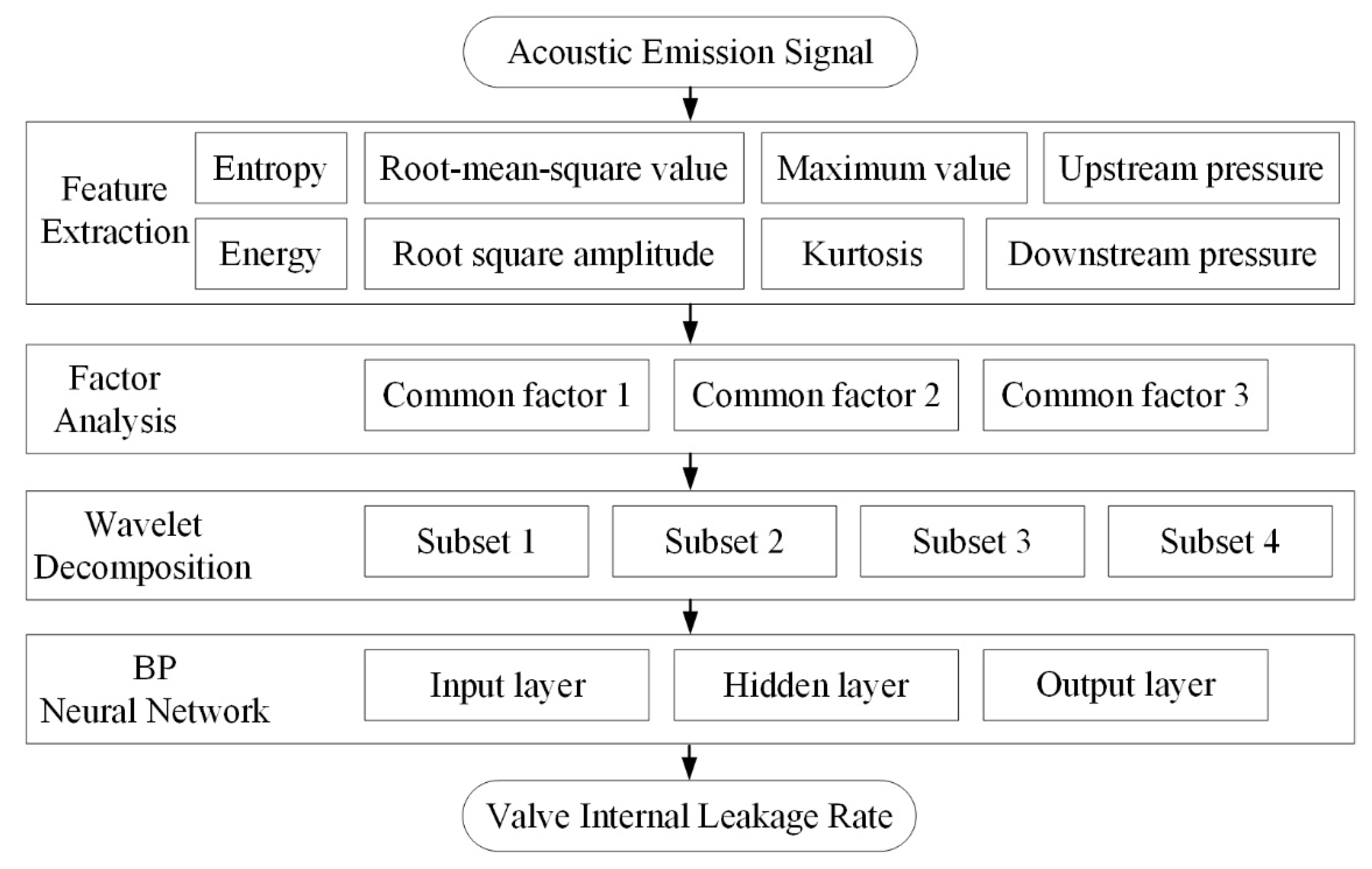
In this study, the AE signals of the internal leakage in a valve are acquired for leakage rate prediction. The novel valve leakage rate prediction method is based on AE technology, factor analysis, wavelet decomposition and BP neural network. Figure 4 describes its procedure, which can be summarized as the following steps:

Step 1: AE signals of the valve internal leakage are collected by the AE system.

Step 2: Eight feature parameters of the AE signal, including entropy, energy, maximum value, root mean square value, root square amplitude, kurtosis, upstream and downstream pressures, are extracted.

Step 3: Factor analysis is used to realize the dimensionality reduction of the AE signals.

Step 4: Wavelet decomposition is performed to obtain four decomposed feature subsets.

Step 5: The BP neural network model is established to predict the valve internal leakage rate.

Step 6: The valve internal leakage rate is obtained.

4.2. Dimensionality Reduction of Acoustic Emission Signals by Factor Analysis

Six parameters were extracted from the acoustic emission signals collected in the experiment, including entropy, energy, maximum value, root mean square value, root square amplitude and kurtosis. Meanwhile, the upstream and downstream pressures corresponding to each signal were also recorded. These high-dimensional features contain a lot of redundant features. If regression prediction analysis is conducted directly, it will be time-consuming and the prediction accuracy will be low. Therefore, before quantitative evaluation of the leakage rate, the high-dimensional features of the acoustic emission signal were reduced based on the factor analysis method. It is expected that a few common factors can be used to explain the complex relationship between multiple variables to be observed.

First, the principal component analysis method was used to extract common factors. Because of the strong correlation in the original data structure, the percentages of variance explained by the first three common factors were 69.635%, 13.823% and 8.658%, respectively. The cumulative variance percentages of these three common factors reached 92.116%, indicating that the loss of valve leakage signal characteristic variable data was very limited, and most of the useful information was retained. Therefore, the first three factors were selected as common factors.

Then, the extraction rate analysis was performed on the three extracted common factors. The common factor variances of the factor analysis are given in

Table 2. Common factor variance.

Parameters	Initial Value	Extraction Rate
Entropy	1.000	0.754
Energy	1.000	0.973
Maximum value	1.000	0.983
Root mean square value	1.000	0.990
Root square amplitude	1.000	0.992
Kurtosis	1.000	0.952
Upstream pressure	1.000	0.881
Downstream pressure	1.000	0.844

. It can be seen from Table 2 that the information extraction rate of the five variables—energy, maximum value, root mean square value, square root amplitude and kurtosis—is higher than 95%, indicating that most of the information in the variables were extracted by the common factors. The information extraction rate of upstream pressure, downstream pressure and entropy also reached more than 75%, indicating that the common factors can explain the information of the original sample data commendably. It is shown that the result of factor analysis is effective.

Next, the maximum variance method, a kind of orthogonal rotation method, was used to rotate the three extracted common factors so as to increase their explanation ability. The principal factor analysis method was used to extract the common factor load, and then Kaiser standardized maximum variance method was used to rotate the factor load four times until it converged iteratively. The factor load matrix after rotation is given in

Table 3. Factorial load matrix after rotation.

Parameters	Factor 1	Factor 2	Factor 3
Energy	0.969	0	0
Maximum value	0.935	0	0
Root mean square value	0.924	0	0
Root square amplitude	0.928	0	0
Downstream pressure	0.746	0	0
Entropy	0	0.686	0
Downstream pressure	0	0.924	0
Kurtosis	0	0	0.920

. It can be seen from Table 3 that Factor 1 has a high load on the five variables of energy, maximum value, root mean square value, root square amplitude and downstream pressure, indicating that these five variables can be explained by a common factor. Factor 2 has a high load on the two variables—upstream pressure and entropy, indicating that these two variables can be explained by a common factor. Factor 3 has a high load on the kurtosis variable, indicating that the kurtosis can be explained by Factor 3 alone.

4.3. Quantification of Internal Leakage Rate Based on Wavelet-BP Neural Network

Based on the sample feature set after dimensionality reduction by factor analysis in the previous section, wavelet decomposition was performed first. Wavelet decomposition can not only increase the number of sample feature sets, but also plays a decisive role in improving the prediction accuracy and anti-interference ability of the neural network quantitative model. Three-layer wavelet decomposition was performed on the sample feature set after dimensionality reduction, and finally, four decomposed sample feature subsets were obtained. The four sample feature subsets were inputted into the quantitative model of the valve internal leakage rate.

In order to evaluate the performance of the quantitative model based on neural network for valve leakage rate, mean absolute error (MAE), root mean square error (RMSE) and Pearson’s correlation coefficient (R) are introduced as evaluation indexes, as shown in Equations (7)–(9).

$$\mathrm{MAE}=\frac{1}{N}{\displaystyle \sum _{i=1}^N\left|y_i-{\overline{y}}_i\right|},$$

(7)

$$\mathrm{RMSE}=\sqrt{\frac{1}{N}{\displaystyle \sum _{i=1}^N{\left(y_i-{\overline{y}}_i\right)}^2}},$$

(8)

$$\mathrm{R}=\frac{{\displaystyle \sum _{i=1}^N\left(d_i-\overline{d}\right)\left(y_i-\overline{y}\right)}}{\sqrt{{\displaystyle \sum _{i=1}^N{\left(d_i-\overline{d}\right)}^2}·{\displaystyle \sum _{i=1}^N{\left(y_i-\overline{y}\right)}^2}}},$$

(9)

where N is the number of samples, y_i is the predicted value by the model, $\overline{y}$ is the average of the predicted value by the model, d_i is the sample value, $\overline{d}$ is the average of the sample. The smaller the value of MAE and RMSE, the better the performance of the model. The larger the value of R, the better the performance of the model.

The sample feature set after dimensionality reduction based on factor analysis is chosen as the sample data for establishing the quantitative prediction model of the valve leakage rate. The number of samples is 100. The sample feature set is divided into two parts, the sample training set and the sample test set, which accounts for 75% and 25% of the sample feature set, respectively. In the previous section, three common factors were extracted by factor analysis, and a three-dimensional feature set was obtained by dimensionality reduction. So, the input layer of the neural network prediction model contains three neurons. The output of the model is the valve leakage rate, so the output layer contains one neuron. In training the BP neural network model, the Sigmoid function is used for both the hidden and output nodes. The weight matrix is initialized to be subject to Gauss distribution N(0,1). The bias vector is initialized as 0. The training set is used to optimize the weight matrix and bias vector by reverse iteration. Then, the trial-and-error method was used to test the effect of the number of hidden layers and the number of neurons in each layer on the performance of the model.

Firstly, it is assumed that the model has only one hidden layer. The first hidden layer has only one neuron. In this case, a neural network model was established. The sample training set was used to train the model. When all the parameters of the model were determined, the sample test set was used to test the performance of the model. By analogy, the performance of the model when the first hidden layer has two, three, ..., nine neurons, was tested gradually. Three evaluation indexes, MAE, RMSE and R were used to evaluate the prediction performance of the model. By doing so, the index scores of the model performance for different numbers of neurons are shown in

Table 4. Scores of model evaluation indexes with a single hidden layer at different numbers of neurons.

Numbers of Neurons	MAE	RMSE	R
1	0.476255	0.581045	0.994024
2	0.548971	0.678835	0.988537
3	0.589502	0.713228	0.986409
4	0.627522	0.818928	0.980072
5	0.714719	0.907486	0.977476
6	0.745887	0.889888	0.980421
7	0.684662	0.852834	0.981729
8	0.712839	0.873321	0.979994
9	0.745381	0.950341	0.974458

.

It can be seen from Table 4 that when the model has only one hidden layer, as the number of neurons increases, the values of the model performance evaluation indexes, MAE and RMSE, increase gradually. While the evaluation index R shows a downward trend. When the model has only one hidden layer and only one neuron in the hidden layer, the evaluation scores of the model, MAE, RMSE and R, are 0.476255, 0.581045 and 0.994024, respectively, which is better than the model performance when the number of neurons is other values. Therefore, it can be concluded preliminarily that when the neural network has a hidden layer and the number of hidden layer neurons is one, the model proves the best performance. The optimal structure of the model can be expressed as 3-1-1.

Secondly, it is assumed that the model contains two hidden layers, and the first hidden layer has only one neuron. Similarly, the trial-and-error method was used to determine the optimal structure of the model. Following the steps above, the model performance index scores when the number of neurons in the second hidden layer varying was calculated, as shown in

Table 5. Scores of model evaluation indexes with double hidden layers at different numbers of neurons.

Neural Network Structure	MAE	RMSE	R
1, 1	0.502898	0.621259	0.992559
1, 2	0.606585	0.749687	0.989804
1, 3	0.53966	0.663171	0.991061
1, 4	0.579667	0.718581	0.988168
1, 5	0.543189	0.662200	0.990392
1, 6	0.747555	0.967281	0.973799
1, 7	0.585091	0.741581	0.984737
1, 8	0.711796	0.903873	0.974746
1, 9	0.705377	0.929872	0.974641

.

It can be seen from Table 5 that when the number of neurons in the second hidden layer is 1, the three evaluation indexes of the model, MAE, RMSE and R, have the best scores, 0.502898, 0.621259 and 0.992559, respectively. Therefore, the optimal structure can be expressed as 3-1-1-1. Compared with the optimal structure of the neural network with a single hidden layer, the performance of the model with double hidden layers is relatively low, but it has little difference. So, the hidden layers should increase continually and the trial-and-error verification is still required.

Next, a model containing three hidden layers is established, in which both the first and second hidden layers contain just one neuron. The trial-and-error method was used again to analyze the influence of the number of neurons in the third hidden layer on the performance of the model. The results are shown in

Table 6. Scores of model evaluation indexes with three hidden layers at different numbers of neurons.

Neural Network Structure	MAE	RMSE	R
1, 1, 1	0.461136	0.635044	0.989873
1, 1, 2	0.535604	0.642995	0.992614
1, 1, 3	0.530611	0.621348	0.992587
1, 1, 4	0.490249	0.611622	0.990989
1, 1, 5	0.572641	0.700308	0.986745
1, 1, 6	0.559857	0.699123	0.988644
1, 1, 7	0.785279	1.035246	0.964303
1, 1, 8	0.737673	0.888437	0.977561
1, 1, 9	0.738591	0.951983	0.971771

.

It can be seen from Table 6 that when the model has three hidden layers and the third hidden layer has only one neuron, the MAE index score of the model is the best, thus 0.461136. When the third hidden layer of the model contains four neurons, the RMSE index score of the model is the best, thus 0.611622. When the third hidden layer of the model contains two neurons, the R index score of the model is the best, thus 0.992614. Comprehensively analyzed, when the third hidden layer of the model contains four neurons, the optimal structure of the model can be expressed as 3-1-1-1-4-1. In this structure, the scores of the three evaluation indexes are 0.490249, 0.611622 and 0.990989, respectively, which is weaker than the 3-1-1 structure and better than the 3-1-1-1 structure.

Using the same method, the index scores of the model with four and five hidden layers were calculated in turn. The optimal structural models correspondingly were concluded. The optimal scores of each index of the models after the optimal structure of each hidden layer was obtained are shown in Figure 5.

It can be seen from Figure 5 that as the number of hidden layers of the model increases, the scores of MAE and RMSE show an upward trend, while R shows a downward trend, indicating that the performance of the model is weakening. Therefore, when the model contains only one hidden layer, the structure of the model is optimal. It can be obtained that the optimal structure of the BP neural network model for quantifying the valve leakage rate is 3-1-1, as shown in Figure 6. In the optimal structure, the input layer contains three neurons, including only one hidden layer with only one neuron and the output layer contains one neuron.

4.4. Comparison of Different Quantitative Models for Internal Leakage Rate

Firstly, the effectiveness of sample dimensionality reduction in improving the prediction performance of the model was verified. A wavelet-BP neural network model based on the sample feature set without dimensionality reduction was established, and the optimal structure of the valve leakage rate quantitative model is 8-6-4-1. It means the input layer of the model contains eight neurons; the model contains two hidden layers, of which the first hidden layer contains six neurons, and the second hidden layer contains four neurons; the output layer contains one neuron.

The comparison between the prediction results of the quantitative model of the wavelet-BP neural network based on the sample feature set by dimensionality reduction and without dimensionality reduction is shown in Figure 7.

It can be seen intuitively from Figure 7 that the prediction results of the quantitative model of the valve leakage rate by the wavelet-BP neural network based on the sample feature set reduced by the factor analysis have a high degree of agreement with the actual leakage rate. It is better than the prediction results of the wavelet-BP neural network based on the sample feature set without dimensionality reduction. It can also be seen from the consistency of the prediction results of the test set that the prediction model based on the dimensionality-reduced sample set has a better prediction performance. The main reason is that after the dimensionality reduction process of the sample feature set, the redundant information is removed, the complexity of the model is reduced, and the prediction accuracy is improved. In addition, the wavelet-BP neural network quantitative model based on the sample feature set after factor analysis is less volatile, and the model has better robustness.

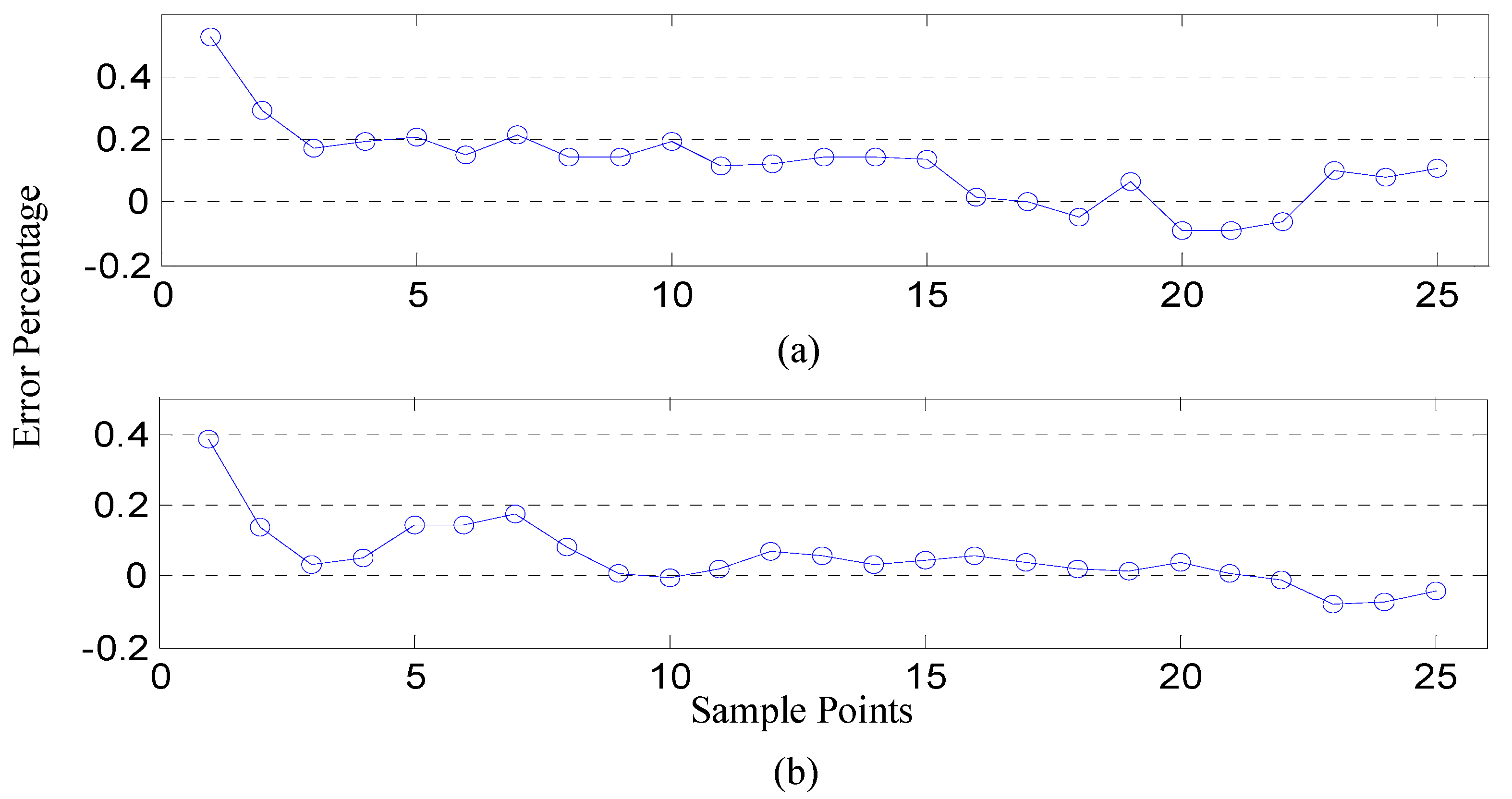
The prediction error of the wavelet-BP neural network model based on the sample feature sets by dimensionality reduction and without dimensionality reduction is shown in Figure 8. It can be seen from Figure 8b that the prediction error of the wavelet-BP neural network model based on the dimensionality-reduced sample feature set is mainly concentrated within ±10%, and only several sample points are greater than 10%, which indicates that the model has a higher prediction accuracy, and less volatility in prediction results. Compared with the wavelet-BP neural network model based on the sample feature set without dimensionality reduction, factor analysis of the sample feature set reduces the dimension, which increases the anti-interference ability of the model and improves the prediction accuracy of the model. It can also be seen from Figure 8b that when the leakage rate is small, the prediction percentage error of the model is significantly larger. The main reason for this is that when the leakage rate is small, the noise of the signal is relatively small, and the deviation caused by noise is large. Besides, under the same condition that the relative errors are consistent, the smaller the reference leakage rate, the greater the percentage error.

Secondly, the effectiveness of wavelet decomposition on the performance improvement of the quantitative model of the internal leakage rate was verified. For the sample feature set without wavelet decomposition, the optimal structure of the quantitative model for the valve internal leakage rate is 3-1-2-1. It means the input layer has three neurons; the first hidden layer has one neuron and the second hidden layer has two neurons; the output layer has one neuron.

The comparison between the prediction results of the quantitative model of the wavelet-BP neural network and BP neural network based on the sample feature set after dimensionality reduction is shown in Figure 9.

As can be seen from Figure 9, the prediction results of the quantitative model of the internal leakage rate based on the wavelet-BP neural network have a high degree of agreement with the actual leakage rate, and the prediction results are significantly better than that of the BP neural network model. Moreover, the prediction results of the wavelet-BP neural network model fluctuate gently, while the prediction results of the BP neural network model fluctuate sharply, indicating that the wavelet-BP neural network model has better robustness. The advantages of wavelet decomposition mainly lie in that the wavelet decomposition of the sample increases the number of sample sets, which makes the error of the model prediction results smaller and the predicted rate closer to the actual rate. Because of the three-layer wavelet decomposition of the sample set, the prediction results of the quantitative model established by the wavelet-BP neural network are less volatile, and the model is more robust.

The prediction errors of the wavelet-BP neural network model and the BP neural network model based on the sample feature set after dimensionality reduction are shown in Figure 10. It can be seen from Figure 10b that the prediction error of the quantitative model based on the BP neural network fluctuates within ±20% as a whole, which has a larger error. This shows that the wavelet decomposition of the sample feature set increases the anti-interference ability of the model, providing the wavelet-BP neural network quantitative model with good prediction performance.

Finally, a comprehensive comparison is made between the prediction results of the wavelet-BP neural network model after dimensionality reduction, the prediction results of the wavelet-BP neural network model without dimensionality reduction, and the prediction results of the BP neural network model after dimensionality reduction. The scores of the evaluation indexes, MAE, RMSE and R, are shown in

Table 7. Index scores of three models.

Models	MAE	RMSE	R
Wavelet-BP neural network model after dimensionality reduction	0.476255	0.581045	0.994024
Wavelet-BP neural network model without dimensionality reduction	1.0261	1.1005	0.9764
BP neural network model after dimensionality reduction	1.1916	1.2974	0.9501

. For the prediction results of the wavelet-BP neural network model after dimensionality reduction, the MAE, RMSE and R indexes are 0.476255, 0.581045 and 0.994024 respectively, which are far superior to the other two models, showing the best prediction performance.

5. Conclusions

This paper proposed an effective method for predicting the internal leakage rate of natural gas pipeline valves. The proposed method combines the advantage of factor analysis in reducing the dimensionality of AE signal sharply and the advantage of wavelet-BP neural network in improving the prediction accuracy and in resisting interference. The extraction rate of the three common factors obtained by factor analysis based on dimensionality reduction for the acoustic emission data reached more than 75%, and the load between the eight original sample parameters and the common factor almost reached more than 90%. This proves the effectiveness of factor analysis. The comparison of models with dimensionality reduction and without dimensionality reduction proves the advantage of factor analysis. The comparison of models with wavelet-BP neural network and BP neural network proves the advantage of wavelet decomposition. The prediction results show that the wavelet-BP neural network quantitative model based on the sample feature set after dimensionality reduction by factor analysis has a high prediction accuracy and a strong anti-interference ability. It can be used as a quantitative model for the prediction of the internal leakage rate in gas pipeline valves, which provides technical support and guarantees the safe operation of valves in gas transmission stations.

References

1. Pan, S.; Xu, Z.; Li, D.; Lu, D. Research on Detection and Location of Fluid-Filled Pipeline Leakage Based on Acoustic Emission Technology. Sensors 2018, 18, 3628. [Google Scholar] [CrossRef] [PubMed] [Green Version]
2. Murvay, P.-S.; Silea, I. A survey on gas leak detection and localization techniques. J. Loss Prev. Process. Ind. 2012, 25, 966–973. [Google Scholar] [CrossRef]
3. Datta, S.; Sarkar, S. A review on different pipeline fault detection methods. J. Loss Prev. Process. Ind. 2016, 41, 97–106. [Google Scholar] [CrossRef]
4. Lee, S.G.; Park, J.H.; Yoo, K.B.; Lee, S.K.; Hong, S.Y. Evaluation of internal leak in valve using acoustic emission method. Key Eng. Mater. 2006, 326, 661–664. [Google Scholar] [CrossRef]
5. Thompson, G.; Askari, A.R. Air leak detection through ball plug valves by vibration monitoring. Noise Vib. Control 1986, 17, 140–143. [Google Scholar]
6. Thompson, G.; Zolkiewski, G. An experimental investigation into the detection of internal leakage of gases through valves by vibration analysis. Proc. Inst. Mech. Eng. Part E J. Process. Mech. Eng. 1997, 211, 195–207. [Google Scholar] [CrossRef]
7. Juvik, T.; Hermansen, T.; Carr, R.; Hale, S. Online valve monitoring systems used on off-shore platforms in the North sea. In Proceedings of the International Conference on Offshore Mechanics and Arctic Engineering, Oslo, Norway, 23–28 June 2002; Volume 36126, pp. 333–337. [Google Scholar]
8. Sohaib, M.; Islam, M.; Kim, J.; Jeon, D.-C.; Kim, J.-M. Leakage Detection of a Spherical Water Storage Tank in a Chemical Industry Using Acoustic Emissions. Appl. Sci. 2019, 9, 196. [Google Scholar] [CrossRef] [Green Version]
9. Duong, B.P.; Kim, J.; Kim, C.-H.; Kim, J.-M. Deep Learning Object-Impulse Detection for Enhancing Leakage Detection of a Boiler Tube Using Acoustic Emission Signal. Appl. Sci. 2019, 9, 4368. [Google Scholar] [CrossRef] [Green Version]
10. Duong, B.P.; Kim, J.; Jeong, I.; Kim, C.H.; Kim, J.-M. Acoustic Emission Burst Extraction for Multi-Level Leakage Detection in a Pipeline. Appl. Sci. 2020, 10, 1933. [Google Scholar] [CrossRef] [Green Version]
11. Kaewwaewnoi, W.; Prateepasen, A.; Kaewtrakulpong, P. Measurement of valve leakage rate using acoustic emission. In Proceedings of the International Conference on Electrical Engineering/Electronics, Computer, Telecommunications, and Information Technology (ECTI’05), Kunming, China, 10–14 July 2005; pp. 597–600. [Google Scholar]
12. Kaewwaewnoi, W.; Prateepasen, A.; Kaewtrakulpong, P. Investigation of the relationship between internal fluid leakage through a valve and the acoustic emission generated from the leakage. Measurement 2010, 43, 274–282. [Google Scholar] [CrossRef]
13. Prateepasen, A.; Kaewwaewnoi, W.; Kaewtrakulpong, P. Smart portable noninvasive instrument for detection of internal air leakage of a valve using acoustic emission signals. Measurement 2011, 44, 378–384. [Google Scholar] [CrossRef]
14. Meland, E.; Henriksen, V.; Hennie, E.; Rasmussen, M. Spectral analysis of internally leaking shut-down valves. Measurement 2011, 44, 1059–1072. [Google Scholar] [CrossRef]
15. Heo, G.; Lee, S.K. Internal leakage detection for feed water heaters in power plants using neural networks. Expert Syst. Appl. 2012, 39, 5078–5086. [Google Scholar] [CrossRef]
16. Meland, E.; Thornhill, N.F.; Lunde, E.; Rasmussen, M. Quantification of Valve Leakage Rates. AIChE J. 2012, 58, 1181–1193. [Google Scholar] [CrossRef] [Green Version]
17. Ye, G.Y.; Xu, K.J.; Wu, W.K. Standard deviation based acoustic emission signal analysis for detecting valve internal leakage. Sens. Actuator A Phys. 2018, 283, 340–347. [Google Scholar] [CrossRef]
18. Zhu, S.B.; Li, Z.L.; Zhang, S.M.; Liang, L.L.; Zhang, H.F. Natural gas pipeline valve leakage rate estimation via factor and cluster analysis of acoustic emissions. Measurement 2018, 125, 48–55. [Google Scholar] [CrossRef]
19. Zhu, S.B.; Li, Z.L.; Zhang, S.M.; Zhang, H.F. Deep belief network-based internal valve leakage rate prediction approach. Measurement 2019, 133, 182–192. [Google Scholar] [CrossRef]
20. Sim, H.Y.; Ramli, R.; Saifizul, A.; Soong, M.F. Detection and estimation of valve leakage losses in reciprocating compressor using acoustic emission technique. Measurement 2020, 152, 107315. [Google Scholar] [CrossRef]
21. Ye, G.Y.; Xu, K.J.; Wu, W.K. Multivariable modeling of valve inner leakage acoustic emission signal based on Gaussian process. Mech. Syst. Signal. Proc. 2020, 140, 106675. [Google Scholar] [CrossRef]
22. Dunegan, H.L. Modal analysis of acoustic emission signals. J. Acoust. Emiss. 1997, 15, 53–61. [Google Scholar]
23. Mostafapour, A.; Davoodi, S. A theoretical and experimental study on acoustic signals caused by leakage in buried gas-filled pipe. Appl. Acoust. 2015, 87, 1–8. [Google Scholar] [CrossRef]
Figure 1. Schematic diagram of the wavelet decomposition principle.
Applsci 10 05544 g001
Figure 2. Model of the backpropagation (BP) neural network.
Applsci 10 05544 g002
Figure 3. Experimental platform for detection valve internal leakage in the gas pipeline.
Applsci 10 05544 g003
Figure 4. Block diagram of the valve internal leakage rate prediction method.
Applsci 10 05544 g004
Figure 5. Evaluation indexes of models with different hidden layers: (a) MAE varies with the number of hidden layers; (b) RMSE varies with the number of hidden layers and (c) R varies with the number of hidden layers.
Applsci 10 05544 g005
Figure 6. Optimal structure of the wavelet-BP neural network prediction model for valve internal leakage.
Applsci 10 05544 g006
Figure 7. The influence of dimensionality reduction on model prediction results.
Applsci 10 05544 g007
Figure 8. Comparison of the influence of dimensionality reduction on model prediction error: (a) prediction error of the wavelet-BP neural network model without dimensionality reduction and (b) prediction error of the wavelet-BP neural network model after dimensionality reduction.
Applsci 10 05544 g008
Figure 9. The influence of the wavelet decomposition on model prediction results.
Applsci 10 05544 g009
Figure 10. Comparison of the influence of wavelet decomposition on model prediction error: (a) prediction error of the wavelet-BP neural network model after dimensionality reduction and (b) prediction error of the BP neural network model after dimensionality reduction.
Applsci 10 05544 g010