Study on Prediction and Application of Initial Chord Elastic Modulus with Resonance Frequency Test of ASTM C 215

Abstract

For accurate design, construction, and maintenance, it is important to identify the elastic modulus of concrete. This is usually achieved using a destructive test based on American Society for Testing and Materials (ASTM) C469. However, obtaining an appropriate static elastic modulus (Ec) requires many specimens, and the testing is difficult and time-consuming. Thus, a dynamic elastic modulus (Ed) is often obtained through a natural frequency for a specific size (e.g., the longitudinal (LT) or transverse (TR) mode) based on a resonance frequency test. However, this method uses a gradient at a very low-stress part of the stress–strain curve and assumes a completely elastic body. In fact, the initial chord elastic modulus (Ei) of the stress–strain curve in a concrete fracture test differs from the Ed, owing to the non-homogeneity and inelasticity of the concrete. The Ei of the experimental value may be more accurate. In this study, the Ei was predicted using machine learning methods for natural frequencies. The prediction accuracy for Ei was analyzed based on f1–f4, as calculated through the LT and TR modes. The predicted Ei had higher correlations with the actual Ec and compressive strength (fc) than Ed. Thus, more accurate prediction of concrete mechanical properties is possible.

1. Introduction

The elastic modulus of concrete is an important factor for the trustworthy design, construction, and maintenance of structures, and can predict the deformation in an actual stress state [1,2]. The static elastic modulus (Ec) of concrete uses the secant elastic modulus of the stress–strain curve as obtained by ASTM C469. However, a large number of specimens is required to obtain a reliable representative value, and it is difficult to provide a sufficient assessment, owing to constraints on time and the difficulty of testing [3,4]. One alternative method comprises obtaining a dynamic elastic modulus (Ed), while resonance frequency test and ultrasonic pulse velocity method can be applied according to ASTM C215 and ASTM C597, respectively [5,6]. Among ultrasonic test methods, a pressure wave (P-wave) measurement provides easy and convenient testing, but the distribution of the data is large, owing to uneven distributions of aggregates, moisture, and voids in the test piece. In addition, although a large correlation between Ec and compressive strength (fc) has been reported as a result of using a shear wave (S-wave), which has a larger energy than a P-wave, it is difficult to measure and obtain consistent data (especially at low ages), owing to the influences of voids and moisture in the concrete [7,8,9,10]. The resonance frequency test is known for consistently predicting the Ed with less fluctuation in the collected data, as it is simple to measure and grasps the overall dynamic characteristics of the specimen. The resonance frequency test assumes that the concrete has a homogeneous elastic modulus, density, Poisson’s ratio, etc., and uses a method to calculate a theoretical elastic modulus for an initial stress range [6,11]. In the ASTM, the relationship between the dynamic modulus for the longitudinal (LT) and transverse (TR) modes was proposed using physical parameters such as the dimensions, mass, and first resonance frequency (f1) [6]. Subramaniam et al. applied f1 and the second resonance frequency (f2) of the LT mode in the Rayleigh Ritz theory, proposing a general equation for the Ed and dynamic Poisson’s ratio [11]. The Eds measured by these non-destructive examination (NDE) methods were larger than the value of Ec, and several empirical equations for predicting Ec through a certain reduction in the Ed ratio have been proposed [12,13,14]. However, the Ed measured according to the NDE method has a large deviation and degree [10]. In addition, the Ed measured with the resonance frequency test has been assumed to be the initial chord elastic modulus (Ei), owing to the deformation of an initial very small stress in the stress-strain curve. Nevertheless, concrete is a nonhomogeneous, inelastic material, and thus the value of Ed as measured with the theoretical equation such as ASTM’s is different from the actual Ei value [10]. In previous studies, the Ei was defined as a slope in the range of 10–50 μ in the stress-strain curve, and was compared to Ed and Ec. The modulus of elasticity was Ed > Ei (10 μ–50 μ) > Ec, and it was determined that there was a difference of 11.62% between the Ec and Ei. [15]. However, if the range of Ei is set to (10–50 μ) as in the previous studies, the correlation with Ec may be small, as the measured value in the initial part of the stress-strain curve is unstable, and has high variation [9,16]. Therefore, if the correct Ei value is extracted, the correlation of Ei–Ec is expected to be greater than that of Ed–Ec. To overcome the limitations of the fracture test and predict Ec more accurately, a non-destructive method for accurately predicting Ei is required.

In recent years, studies have been conducted to overcome the nonlinearity and improve the prediction accuracy of the mechanical properties (such as the Ec and fc) of concrete by considering various variables such as the water/binder ratio, type of binders/aggregates and corresponding ratios by machine learning (ML), rather than by general regression analysis. These studies focused on predicting the concrete strength and integrity more accurately with general ML algorithms, such as the support vector machine (SVM), ensemble and artificial neural network (ANN), and provided predictions with relatively improved accuracy [17,18,19,20]. For example, Erdal et al. used ensemble and ANN methods with cement, blast-furnace slag, water, and aggregate, and compared the accuracies of fc prediction for high-performance concrete; they found that the ensemble method was slightly better [21]. Park et al. predicted the Ec and fc using four Eds with SVM, ensemble, ANN, and multiple linear regression (MLR) methods, and announced that the ensemble and ANN were suitable [8]. Yan and Shi predicted the Ec by the fc using an ANN, SVM, linear regression, and four theoretical equations, and reported that the ML methods were more suitable than linear regression and theoretical equations [22]. Young et al. used an ANN, SVM, and linear regression to predict a 28-day intensity from data with varying mixing ratios and reported that ML methods were more accurate than linear regression [23]. Cihan used ANN, ensemble, and SVM methods to estimate the fc and slump values of concrete and reported that the ANN and ensemble approaches were superior to the SVM [24]. Among the ML methods, the ANN and ensemble methods overcome the nonlinear behavior of concrete and provide suitable contributions to quality prediction. However, although some studies have been conducted on the prediction of Ec and fc with Ed, few studies have been conducted with Ei. Therefore, it is necessary to analyze the relationships among Ed, Ec, and fc for the application of Ei, and to predict the correct Ei.

In this study, the difference between the dynamic elastic modulus (Ed) and initial chord elastic modulus (Ei) values obtained with the ASTM theoretical equation was analyzed based on the results of the resonance frequency test, and the relationship between the Ec and fc was analyzed through accurate prediction of the Ei. Three Ed values were obtained using the theoretical equations suggested by ASTM C215-14 and Subramaniam, as the frequencies of the LT and TR modes of the resonance frequency test. In addition, the exact Ei value at the origin was extracted through curve fitting to the stress–strain curve, and was compared with the Eds. The Ei was predicted using ML (ensemble, ANN) for the frequency, and the Ed was obtained by the resonance frequency test. In addition, the contributions of the variables were analyzed. The ML method was trained on several combinations, and a five-fold cross validation was performed to prevent the overfitting of the predicted results. The mean squared error (MSE) and mean absolute percentage error (MAPE) were used to analyze the errors between the predicted and actual Ei values. In addition, the relationships with the Ec and fc were analyzed to confirm the predicted possibility of using the Ei.

2. Materials and Methods

2.1. Materials and Preparation of Specimens

The concrete consisted of Type I Portland cement, river sand, supplementary cementitious materials (SCMs), and crushed granite (up to 25 mm in size). The concrete in this study replaced approximately 50% of the cement with granulated blast furnace slag (GBFS) and fly ash. It possessed high strength in the long term, but the initial strength development could be slow. Two concrete mixtures (Mix 1, Mix 2) were prepared with W/B ratios of 0.45 and 0.35, respectively, and were expected to develop fcs of 20 and 40 MPa at 28 days, respectively. The ratios of concrete mixture are summarized in

Table 1. Proportions of the concrete mixture groups ¹.

ID	Cement Type	W/B	S/A	W	C	S	G	Unit Quantity (kg/m3) Mineral Admixture		Chemical Admixture
								FA	GBFS	AE (Binder%)	SP (Binder%)
Mix1 (20 MPa)	Type I	0.45	0.46	259	121	777	934	58	69	0.9	-
Mix2 (40 MPa)		0.35	0.47	308	166	761	886	81	85	-	1

¹ SCMs: Supplementary cementitious materials, W: water, C: cement, S: sand, G: crushed cobblestone, FA: fly ash, SC: slag cement, AE: air-entraining agent, SP: superplasticizer, GBFS: granulated blast furnace slag.

. 300 cylinders were cast to a size of 150 × 300 mm according to ASTM C31/C31M-12 [25]. The Ec, fc, and Ed values were tested at different ages, i.e., 4, 7, 14, and 28 days. The 28-day fcs for the Mix1/Mix2 cylinders were 19.26 MPa /43.99 MPa, similar to the expected fc.

2.2. Destructive Tests for Elastic Modulus and Compressive Strength

For the measurement of the static elastic modulus (Ec) and compressive strength (fc), each cylinder was positioned vertically, with both ends polished, and the protrusions on the specimen surface removed. As shown in Figure 1, the Ec and fc for each concrete cylinder were measured with a universal testing machine (UTM, Instruments, Instron, MA, USA) with a capacity of 1000 kN, according to ASTM C39/C39M-14a and ASTM C469/C469M-14 [3,26]. The UTM was operated at a speed of approximately 0.28 MPa/s.

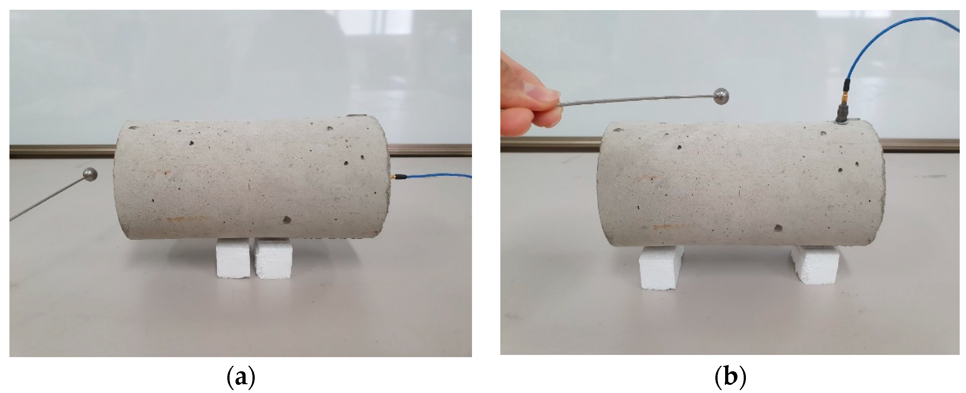
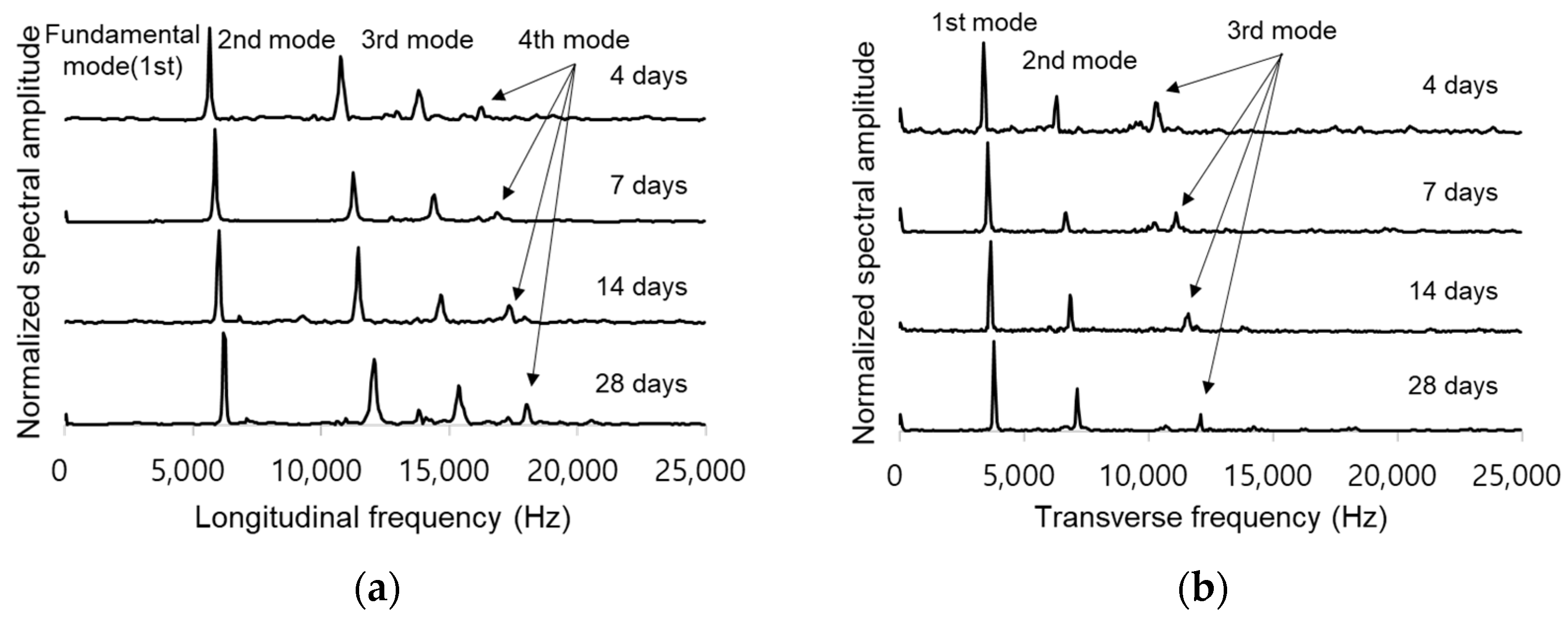
2.3. Dynamic Elastic Modulus Measurements with Resonance Frequency Tests

As shown in Figure 2, the three to four longitudinal and transverse resonance frequencies of the concrete cylinders were measured based on ASTM C215-14 [6]. A steel ball hammer with a diameter of 10 mm was used to generate stress waves in the concrete cylinder. This hammer was suitable for generating very low to 20 kHz frequency signals. An accelerometer (PCB 353B16, PCB, Depew, NY, USA) with a resonance frequency of approximately 70 kHz was used to measure the dynamic response of the concrete cylinders. The time signals measured with the accelerometer were stabilized by a signal conditioner (PCB 482C16, PCB, Depew, NY, USA) and were digitized with 1 MHz sampling through an oscilloscope (NI-PXIe 6366). The time signals were transformed into the frequency domain by a fast Fourier transform algorithm.

Figure 3 shows typical spectral amplitudes of the concrete cylinders at 4, 7, 14, and 28 days in the Mix 2 cylinder. The resonance frequency appears as a large amplitude in the amplitude spectrum. The most dominant frequency was considered as the basic resonance frequency of the longitudinal $f_{LT}$ and transverse $f_{TR}$ modes, with four resonance frequencies in the LT mode and three resonance frequencies in the TR mode. The first of these frequency values was used to calculate the Ed of the LT and TR modes, using Equations (1) and (2) from ASTM C215-14.

$$ASTM.LT={\alpha }_{LT}m{f}_{LT}^2\left(Pa\right)$$

(1)

$$ASTM.TR={\alpha }_{TR}m{f}_{TR}^2\left(Pa\right)$$

(2)

In the above, ASTM.LT and ASTM.TR are the Ed values calculated with $f_{LT}$ and $f_{TR}$, respectively, as the first resonance frequencies. ${\alpha }_{LT}$ has a constant value with regard to the dimensions of the specimen (=5.093 × ($L/d^2$)), where d is the diameter and L is the length. ${\alpha }_{TR}$ has a constant value with regard to Poisson’s ratio and the size of the cylinders (=1.6067 × ($L^{3}T/d^4$)). T is a correction factor corresponding to the Poisson’s ratio, and m is the mass of the cylinders in kg [6].

In addition, as in the method of predicting the dynamic elastic modulus (Ed) with two frequencies as proposed by Subramaniam et al., the dynamic Poisson’s ratio was obtained through Equation (3), and the Ed was predicted through Equation (4).

$$\mu =A_1{\left(\frac{f_2}{f_1}\right)}^2+B_1\left(\frac{f_2}{f_1}\right)+C_1$$

(3)

$$f1,f2.LT=2\left(1+\mu \right)\rho {\left(\frac{2\pi f_1{R}_0}{f_n^1}\right)}^2$$

(4)

Here, $f_1,f_2.LT$ is the Ed value calculated with $f_1$ and $f_2$, $f_1$ is the first frequency, $f_2$ is the second frequency, $R_0$ is the diameter of the cylinder, $A_1$, $B_1$, and $C_1$ are correction factors, $\rho$ is the density, and $f_n^1$ is a correction factor based on the dynamic Poisson’s ratio [11].

2.4. Initial Chord Elastic Modulus Measurement

To calculate the initial chord elastic modulus (Ei) from the measured stress and strain data, a predictive equation for the stress-strain curve of the existing concrete (such as Equations (5) and (6)) can be used [27,28]. However, the existing theoretical equations are suitable for hardened concrete; when measuring the slope of the 10 μ and 50 μ strain ranges applied in previous studies, the initial data value was unstable, and the variability was large. Thus, the error could be large. Therefore, as shown in Figure 4, instead of extracting the Ei with an existing theoretical equation, the curve was predicted through best curve fitting from the origin to the max fc′, and the slope of Ei was calculated from the origin.

$$fc=\frac{2{fc}^{\prime }\left(\frac{x}{\epsilon ce}\right)}{1+{\left(\frac{x}{\epsilon ce}\right)}^2}$$

(5)

$$fc={fc}^{\prime }\left[2\left(\frac{x}{\epsilon ce}\right)-{\left(\frac{x}{\epsilon ce}\right)}^2\right]$$

(6)

3. Machine Learning Methods

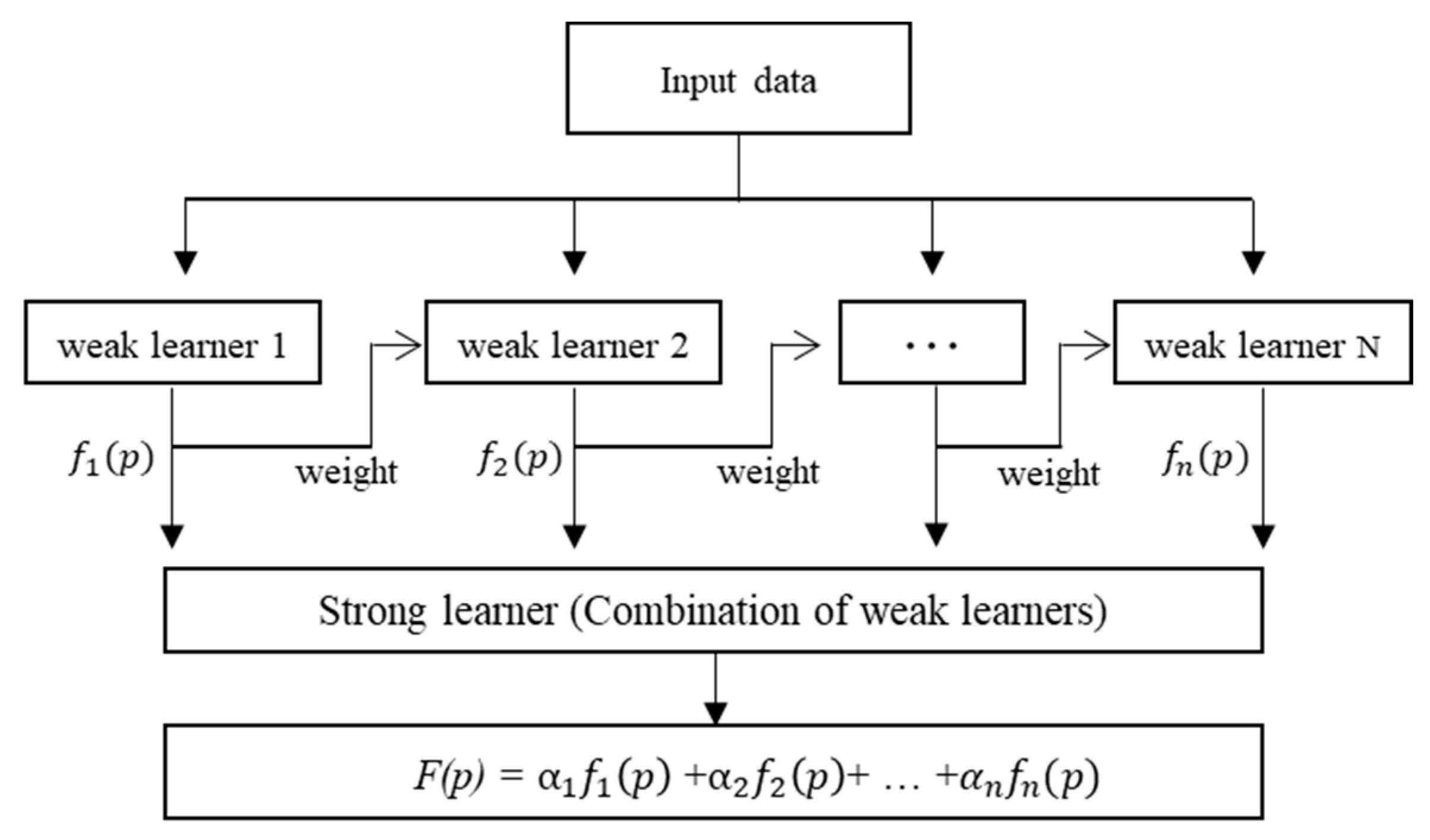
3.1. Ensemble Method

The ensemble method combines several weak learners to create learners with strong predictive power. This study used a regression tree ensemble method and boosting method to combine weak learners. The boosting method performs slightly better than a bagging method and shows a higher predictive power. In addition, the boosting method can compensate for weaknesses in learning the next regression tree, by assigning weights to reduce the error between the predicted and output values of the previously learned regression tree. Here, a least squares method was to calculate the error. As shown in Figure 5, least squares boosting (LSBoost) is a sequential ensemble method that sequentially builds a decision tree. It works in a way that compensates for errors in the previous tree and is defined as shown in Equation (7) [29,30].

$$F_T\left(x\right)={\displaystyle \sum }_{t=1}^T{f}_t\left(p\right)$$

(7)

Here, x, $f_t$, and $F_T\left(p\right)$ represent the input variable, weak learner, and strong learner, respectively.

Each weak learner produces an output which is a hypothesis for each sample of the training set. One weak learner is selected in each repetitive step t. Then, a coefficient is allocated to minimize the sum of the training errors at the final t-step acceleration classifier, as follows (Equation (8)):

$$E_t={\displaystyle \sum }_{i}E\left[F_{t-1}\left(p_i\right)+{\alpha }_{t}h(p_i\right)]$$

(8)

In the above equation, $F_{t-1}\left(p\right)$ and $E\left(F\right)$ are the accelerated learners and error functions generated up to the previous training stage, respectively, and $f_t\left(p\right)={\alpha }_{t}h\left(p\right)$ is weak learner considered for the final learner. In each iteration step of the training process, a weight of a value equal to the current error $E\left(F_{t-1}\left(p_i\right)\right)$ for the training data set is reflected in the next data set, thereby compensating for the error.

3.2. Artificial Neural Network (ANN)

An ANN is a statistical learning algorithm based on a biological neural network, i.e., its structure and function. ANNs make use of connected artificial neurons and perform nonlinear modeling through neurons explaining their unique behaviors by learning input parameters. The multilayer perceptron (MLP) is the most commonly employed ANN architecture; it is comprised of input, hidden, and output layers, as shown in Figure 6 [31]. As shown in Equation (9), all the neurons connected in every layer of the ANN include weights (w) and biases (b). In addition, the neuron values of the previous layers are modified by various weights and compensated through biases.

$$y_i=f\left(net\right)=f\left({\displaystyle \sum }_{i=1}^n{\omega }_i{p}_i+b_j\right)$$

(9)

In the above, p is the input value (i = 1, …, n), b denotes the bias of the neuron, w denotes the weight vector between neurons, f is the activation function, and y represents the output value. An MLP is ordinarily trained using an inverse propagation algorithm, where interconnected weights in the network are repeatedly adjusted to minimize errors (defined as root mean square errors) (RMSEs) [32]. Previous studies have reported that the Levenberg–Marquardt algorithm is suitable as it produces coherent results for the majority of ANNs [33].

4. Results and Discussion

4.1. Experimental Consistency of Static and Dynamic Tests

The static elastic modulus (Ec), initial chord elastic modulus (Ei), and compressive strength (fc) values were collected through static testing of the concrete according to ASTM C469/C469M-14 and ASTM C39/C39M-14a [3,26], and the Eds (ASTM.LT, f1,f2.LT, and ASTM.TR) values calculated as the first and second resonance frequencies were calculated using Equations (1)–(4), for frequencies obtained by dynamic testing according to ASTM C215-14. The ranges of physical and mechanical properties of the specimens in the Mix1 and Mix2 were summarized in

Table 2. The range of physical and mechanical properties in the Mix 1 and 2.

w/c	The Number of Specimens	Weight (kg)	Dimension		Density (kg/m3)	Age (Day)	fc (MPa)	Ec (MPa)
			Diameter (mm)	Length (mm)
0.45 (Mix1)	91	10.66 ~12.12 (11.19)	150 ~150 (150)	290.95 ~298.10 (293.97)	2051.58 ~2340.38 (2153.14)	4	7.33~8.56 (7.91)	9202~15,929 (10,368)
						7	9.31~10.85 (10.07)	10,930~13,256 (11,784)
						14	12.67~14.63 (13.87)	12,723~16,883 (14,735)
						28	17.65~20.68 (19.26)	14,552~20,915 (17,041)
0.35 (Mix2)	194	11.10 ~12.08 (11.63)	150 ~150 (150)	293.30 ~299.70 (297.50)	2125.88 ~2290.24 (2212.76)	4	20.96~26.19 (24.12)	14,566~23,879 (16,796)
						7	27.21~32.56 (29.62)	15,431~19,807 (18,079)
						14	32.82~42.38 (38.17)	15,523~24,009 (20,904)
						28	40.21~47.34 (43.99)	18,686~26,530 (22,860)

and the coefficient of variation (COV) which means the standard deviation (σ) divided by the mean value (μ) of the same group was used to evaluate the consistency of the test results in

Table 3. Summary of statistical analysis.

Days/Variable		ASTM.LT [MPa]		f1f2.LT [MPa]		ASTM.TR [MPa]		Ei [MPa]		Ec [MPa]		fc [MPa]
		Mix 1	Mix 2	Mix 1	Mix 2	Mix 1	Mix 2	Mix 1	Mix 2	Mix 1	Mix 2	Mix 1	Mix 2
Day 4	N	24	49	24	49	24	49	24	49	24	49	24	49
	μ	15,378	24,348	15,643	24,813	14,850	23,914	10,745	18,650	10,368	16,796	7.91	24.12
	COV	4.36%	3.81%	4.71%	4.00%	4.56%	4.01%	7.89%	7.36%	14.31%	7.84%	4.29%	5.10%
Day 7	N	19	49	19	49	19	49	19	49	19	49	19	49
	μ	17,643	26,166	18,003	26,561	17,151	25,294	13,301	20,467	11,784	18,079	10.07	29.62
	COV	4.30%	2.39%	4.36%	2.57%	5.16%	2.71%	4.36%	4.31%	4.90%	4.60%	4.57%	3.03%
Day 14	N	25	50	25	50	25	50	25	50	25	50	25	50
	μ	20,696	28,543	21,057	28,973	20,074	27,530	16,804	24,003	14,735	20,904	13.87	38.17
	COV	3.72%	2.47%	3.80%	2.64%	3.88%	3.01%	5.35%	5.81%	6.10%	6.96%	3.35%	5.47%
Day 28	N	23	46	23	46	23	46	23	46	23	46	23	46
	μ	23,814	30,348	24,239	30,805	22,959	29,652	19,648	25,853	17,041	22,860	19.26	43.99
	COV	3.94%	2.14%	4.35%	2.35%	3.92%	2.73%	6.25%	4.90%	6.88%	6.21%	4.09%	4.32%

. Outliers were detected using the Z-score method, and some data were removed from the statistical analysis [34]. The COV of the Ec by static testing ranged from 4.60% to 14.31%, and the COV of the fc ranged from 3.03% to 5.47%. The 28-day fc values of Mix1 and Mix2 were 19.26 MPa and 43.99 MPa, respectively, i.e., similar to the target fc. However, the COV of the Ec, which was slightly higher in Mix 1 (low curing age), was slightly distorted on the opposite side of the test piece; thus, the deformation during compression was not uniform. This appears to make the Ec more sensitive than the fc in static testing. The COV of the Ei ranged from 4.31% to 7.89%, and by using the method shown in Figure 4, it was possible to overcome the instability in the initial part of the stress–strain curve to collect consistent values. The COV ranges of ASTM.LT and ASTM.TR as measured by the longitudinal and transverse resonance frequency tests were 2.14%–4.36% and 2.71%–5.16%, respectively. The COV of f1f2.LT, in which the first and second frequencies in the longitudinal mode of the resonance frequency test were used, ranged from 2.35% to 4.71%. For ASMT.LT, f1,f2.LT, and ASTM.TR, the COV remained reasonably consistent.

4.2. Relationship among Static and Initial Chord and Dynamic Elastic Modulus

The static elastic modulus (Ec) of concrete can be determined using a dynamic test method. Various empirical equations have been proposed for the prediction of Ec in several studies, using measured Ed values. Popovics considered the density of concrete in the relationship between Ed and Ec and proposed Equation (10) for lightweight concrete and general concrete. ${\omega }_c$ represents the density of hardened concrete (kg/m³) [12].

$$E_c=\frac{446.09E_d{}^{1.4}}{{\omega }_c}\left(\mathrm{MPa}\right)$$

(10)

As another example, the British standard BS8110 Part 2 proposed Equation (11). This equation does not apply to concrete or lightweight aggregate concrete containing more than 500 kg of cement per 1 m³ of concrete [13].

$$E_c=1.25E_d-19000\left(\mathrm{MPa}\right)$$

(11)

Lydon and Balendran proposed an empirical relationship (Equation (12)) between the Ed and Ec [14].

$$E_c=0.83E_d\left(\mathrm{MPa}\right)$$

(12)

The values of dynamic elastic modulus (Ed) as measured by the three methods in Figure 7 were almost similar, and the values followed Eds (f1, f2.LT, ASTM.LT, and ASTM.TR) calculated as the first and second resonance frequencies. Compared to the added empirical equation, the predicted static elastic modulus (Ec) and measured value of do not match, and in fact, the Ed value may vary greatly depending on the test methods and size and type of cylinder. Therefore, it is difficult to select the correct empirical equation for producing the minimum error for the various dynamic tests and cylinders. As expected, the initial chord elastic (Ei) had a large margin of error with the Ed, and was in the middle of the Ed and Ec. In addition, the Ei is less variable and more consistent than the Ed in relation to the Ec.

Table 4. Correlation between static elastic modulus (Ec) and E-modulus.

Correlation	ASTM.LT-Ec	f1,f2.LT-Ec	ASTM.TR-Ec	Initial Chord Elastic Modulus (Ei)-Ec
Value	0.9376	0.9362	0.9364	0.9645

summarizes the correlations between Ed, Ei, and Ec. The correlation between the three Ed values and Ec was 0.93, and Ei and Ec were analyzed to have a greater correlation, at 0.96. Therefore, it is necessary to accurately predict the Ei as having a greater correlation with Ec.

Next, the E-moduli are compared, based on the most commonly used ASTM.LT value among the resonance frequency test for predicting the Ed. By comparing ASTM.LT values, other Eds (ASTM.LT, f1,f2.LT, and ASTM.TR) show linear trend, but the Eds, initial chord elastic modulus (Ei), and static elastic modulus (Ec) have nonlinear relationship. Ei and Ec show similar trends and data distributions; thus, it is more appropriate to use the Ei rather than Eds, according to the theoretical equation for Ec prediction.

In

Table 5. Comparison of errors and correlations between Ei and dynamic elastic moduli (Eds).

Type of Errors	ASTM.LT	f1,f2.LT	ASTM.TR
Mean square error (MSE)	2.53 × 107	2.95 × 107	1.88 × 107
Root MSE (RMSE)	5031	5427	4338
Mean absolute percentage error (MAPE)	26.32%	28.39%	22.59%
R	0.9572	0.9556	0.9551

, the errors and correlations of Ed and Ei are analyzed. MSE, RMSE, and MAPE were used as methods for confirming errors. The MSE and MAPE are defined in Equations (13) and (14), respectively, where n is the number of data, $A_i$ is the Ei value, and $P_i$ is the Ed value.

$$MSE=\frac{1}{n}{\displaystyle \sum }_{i=1}^n{\left(A_i-P_i\right)}^2$$

(13)

$$MAPE=\frac{1}{n}{\displaystyle \sum }_{i=1}^n\left|\frac{A_i-P_i}{A_i}\right|$$

(14)

As the three Eds have almost similar values and trends for the same cylinder, the correlation with Ei was close to 0.95. ASTM.TR had the smallest MAPE with the Ei.

Figure 8 shows the relationships between the ASTM.LT and initial chord elastic modulus (Ei) according to mixes and ages. The MAPEs of the dynamic elastic modulus (Ed) and Ei were large at low age and decreased as age increased. In addition, the difference between the Ed and Ei in Mix 2, a higher strength mixture, was smaller. This trend is considered to decrease the difference between the Ed value and Ei in the theoretical equation, as the moisture content inside the concrete is small (because the w/c ratio is small).

The difference between the dynamic elastic modulus (Ed) and initial chord elastic modulus (Ei) values from the three theoretical equations was confirmed using the method shown in Figure 9, and an analysis was conducted to confirm how accurately the Ei could be predicted by correcting for the Eds. The correction factors and MAPE according to the mixes and ages are summarized in

Table 6. Correction factors and MAPE for ages and mixes between Ed and Ei.

ID	Mix	Day 4	Day 7	Day 14	Day 28	Average
ASTM.LT	Mix 1	0.70 (6.38%)	0.75 (2.81%)	0.81 (3.12%)	0.83 (3.43%)	0.77 (7.47%)
	Mix 2	0.77 (4.69%)	0.78 (3.42%)	0.84 (4.69%)	0.85 (3.19%)	0.81 (5.94%)
f1,f2.LT	Mix 1	0.69 (7.02%)	0.74 (3.35%)	0.80 (3.51%)	0.81 (3.91%)	0.76 (7.63%)
	Mix 2	0.75 (5.54%)	0.77 (4.14%)	0.83 (4.81%)	0.84 (3.24%)	0.80 (6.12%)
ASTM.TR	Mix 1	0.72 (6.25%)	0.78 (4.17%)	0.84 (4.29%)	0.86 (4.79%)	0.80 (7.32%)
	Mix 2	0.78 (4.81%)	0.81 (3.82%)	0.87 (5.28%)	0.87 (4.13%)	0.83 (5.98%)

. Although the MAPE with the Ei could be lowered to 4.69%, 2.81%, 3.12%, and 3.43% (for days 4, 8, 14, 28, respectively) with corrections based on mixes and ages for the Eds values, this process was quite complicated and difficult. Therefore, the entire data were applied for the ASTM.LT, f1,f2.LT, and ASTM.TR, average correction factors of 0.80, 0.79, and 0.82. Compared to the actual Ei value, the MAPE values of ASTM.LT, f1,f2.LT, and ASTM.TR according to the correction factors showed errors of 6.40%, 6.50%, and 6.43%, respectively. However, the Ei is not suitable for predicting the entire section, as it is nonlinear with the theoretical equations.

Next, as a method for predicting the Ei, an analysis was conducted with the fundamentally collected frequencies in the resonance frequency test. Figure 9 shows the relationship between the first resonance frequency in the longitudinal mode and the E-modulus. The first to fourth frequencies are defined as f1 to f4. For f1, the ASTM equation has an exponential function form. The Ei and Ec have the same form. Based on these results, the Ei and Ec could be predicted using the ASTM method (correction coefficient, etc.), and the Ei and Ec could be predicted using the resonance frequencies (such as f1 and f2) collected in the resonance frequency test. Therefore, an analysis was conducted with the f1 to f4 resonance frequencies collected through the resonance frequency test.

Figure 10a shows the relationship between the four frequencies in the longitudinal (LT) mode and initial chord elastic modulus (Ei), and Figure 10b shows the relationship between the three frequencies in transverse (TR) mode and Ei. The number of used data and frequency range for the frequency combination of LT and TR modes are summarized in

Table 7. Summary of used data in the LT mode for machine learning analysis.

Type of Mode	The Number of Specimens	Variable	f1 (Hz)	f2 (Hz)	f3 (Hz)	f4 (Hz)	Weight (kg)	Diameter (mm)	Length (m)	Density (kg/m3)
LT.f1	285	Range	4450 ~6400				10.66 ~12.12	150	290.95 ~299.70	2051.58 ~2340.38
		Average	5641				11.49	150	296.38	2193.72
LT.f2	283	Range		8500 ~12,100			10.66 ~12.12	150	290.95 ~299.70	2051.58 ~2340.38
		Average		10,757			11.49	150	296.39	2193.79
LT.f3	275	Range			10,550 ~15,500		10.66 ~12.12	150	295.00 ~299.40	2051.58 ~2340.38
		Average			13,677		11.50	150	297.41	2194.86
LT.f4	230	Range				12,400 ~20,250	10.66 ~12.12	150	295.00 ~299.60	2051.58 ~2340.38
		Average				15,838	11.48	150	297.68	2191.51
LT.f1,f2	283	Range	4450 ~6400	8500 ~12,100			10.66 ~12.12	150	290.95 ~299.70	2051.58 ~2340.38
		Average	5640	10,757			11.49	150	296.39	2193.79
LT.f1,f2,f3	275	Range	4450 ~6400	8500 ~12,100	10,550 ~15,500		10.66 ~12.12	150	295.00 ~299.40	2051.58 ~2340.38

and

Table 8. Summary of used data in the LT mode for machine learning analysis.

Type of Mode	The Number of Specimens	Variable	f1 (Hz)	f2 (Hz)	f3 (Hz)	Weight (kg)	Diameter (mm)	Length (m)	Density (kg/m3)
TR.f1	285	Range	2750 ~3900			10.66 ~12.12	150	290.95 ~299.70	2051.58 ~2340.38
		Average	3441			11.49	150	296.38	2193.72
TR.f2	105	Range		5150 ~7700		10.71 ~12.12	150	290.95 ~299.50	2069.88 ~2340.38
		Average		6276		11.42	150	295.99	2182.91
TR.f3	105	Range			7750 ~12,250	10.71 ~12.12	150	290.95 ~299.50	2069.88 ~2340.38
		Average			9919	11.42	150	295.99	2182.91
TR.f1,f2	105	Range	2750 ~3850	5150 ~7700		10.71 ~12.12	150	290.95 ~299.50	2069.88 ~2340.38
		Average	3351	6276		11.42	150	295.99	2182.91
TR.f1,f2,f3	105	Range	2750 ~3850	5150 ~7700	7550 ~12,250	10.71 ~12.12	150	290.95 ~299.50	2069.88 ~2340.38
		Average	3351	6276	9919	11.42	150	295.99	2182.91

. The data with unclear peaks or inconsistent with others in the frequency domain were excluded from the analysis. As both the LT and TR modes increased from f1 to f4, the variance of the data increased, and the consistency of data decreased. f1 and f2 of the LT and TR modes have relatively small coefficient of variation (COV) values and are statistically stable, whereas the trend can be identified from f3, but the statistical stability is poor. The ratio of f1, f2, f3, and f4 at the bottom and top of the LT mode was similar to 1.9, 2.43, and 2.82, but in the TR mode, f1-f2 was 1.85, and f1-f3 showed a large error.

Next, the correlation between the frequencies of the LT and TR modes and initial chord elastic modulus (Ei) was analyzed, as shown in

Table 9. Correlation of frequencies and Ei in LT and TR modes.

Correlation	LT.f1-Ei	LT.f2-Ei	LT.f3-Ei	LT.f4-Ei	TR.f1-Ei	TR.f2-Ei	TR.f3-Ei
Values	0.9420	0.9397	0.8629	0.7071	0.9413	0.8992	0.7915

. In the LT mode, the correlation between the frequency and Ei was f1 > f2 > f3 > f4. The correlation values of f1 and f2 were almost identical and had a high correlation with Ei. In the TR mode, f1-Ei had the largest correlation at 0.94, but the correlation greatly decreased from f2. It was confirmed that the Ei can be predicted with f1 and f2 with high correlation, through analysis of the variability of the resonance frequency for each mode and correlation with the Ei.

4.3. Prediction of Initial Chord Elastic Modulus with Multiple Linear Regression

Subramaniam et al. applied f1 and f2 to Equation (3) to obtain a dynamic Poisson’s ratio, and proposed an equation for predicting the Ed through Equation (4) [11]. The multiple linear regression (MLR) results using the LT mode’s f1 and f2 values with high correlations with the Ei and small data variability were compared with those from the theoretical equation of Subramaniam. Equations (15) and (16) for f1, f2, and E-modulus (f1,f2.LT: Ed measured by the first and second frequency in LT modes, Ei) values were extracted using the curve fitting toolbox of MATLB R2019b and were compared in three dimensions, as shown in Figure 11.

$$Ei=-{3.088}^4+4.104\times f1+2.575\times f2$$

(15)

$$f1,f2.LT=-{2.853}^4+11.9\times f1-1.247\times f2$$

(16)

Generally, in the LT mode, f2 has a value of 1.8–2 times f1. The MLR plane has a similar specific gravity to f1 and f2 and has a positive correlation. In the Subramaniam equation, f1 has a high specific gravity and positive correlation, and f2 has a small specific gravity and negative correlation. The MAPE of the Ei as predicted by the MLR with f1 and f2 and actual Ei could be lowered by 5.04%, i.e., higher accuracy than the predicted result through general correction to the theoretical equation.

4.4. Prediction of Initial Chord Elastic Modulus with Ensemble Method

Recently, studies have been conducted to overcome the nonlinearity of data by applying machine learning (ML) methods, and to improve prediction accuracy and reliability. In this study, ML methods are applied to overcome the nonlinearity of data that is difficult to predict using basic regression analysis and correction factors. The errors of the initial chord elastic modulus (Ei) and actual Ei values as predicted by various combinations of frequencies by the ensemble method are summarized in

Table 10. Ei predicted by LT mode frequencies with ensemble.

LT Mode	f1	f2	f3	f4	f1~2	f1~3	f1~4
MSE	1.18 × 106	1.21 × 106	2.75 × 106	4.73 × 106	1.08 × 106	9.74 × 105	9.06 × 105
RMSE	1080	1100	1660	2170	1040	987	952
MAPE	3.90%	3.95%	5.69%	8.00%	3.67%	3.52%	3.51%
R	0.9716	0.9705	0.9332	0.8900	0.9738	0.9768	0.9798

and

Table 11. Ei predicted by TR mode frequencies with ensemble.

TR Mode	f1	f2	f3	f1~2	f1~3
MSE	1.36 × 106	1.64 × 106	1.83 × 106	1.13 × 106	7.74 × 105
RMSE	1160	1280	1350	1060	879
MAPE	4.31%	4.44%	5.79%	3.87%	3.40%
R	0.9668	0.9620	0.9577	0.9740	0.9822

. As a result of the analysis, when a single frequency was used, MAPE values of 3.90% and 4.31% were found for the longitudinal (LT) and transverse (TR) modes, respectively. In the ensemble method, using only f1 can reduce the error by 1–2% more than in the correction coefficient and MLR method. Thus, it is possible to predict a sufficiently accurate Ei value using only f1. As the number of frequencies being used increased, the accuracy tended to increase. In the LT/TR modes, maximum MAPE values of 3.51%/3.40% were shown. Through the correlation analysis shown in Table 10 and the predicted accuracy values in Table 9 and Table 10, approximate contributions to f1 to f4 can be inferred. However, as they are not exact values, an additional contribution analysis was performed.

The relative importance (RI) was calculated using the Statistics and Machine Learning Toolbox of MATLAB R2019b to identify the detailed contribution of each variable from a combination of four frequency variables. As presented in Figure 12 and Figure 13, the results of the contribution analysis showed that f1 was more than 75% in the all combinations and had a dominant effect on the Ei prediction. However, even if the contribution of other factors is low, they can contribute to some prediction accuracy. Also, the difference in the contribution of each variable for each case is due to the data difference, and especially when consistent data from f1 to f4 were used, the contribution of f1 tends to be large.

Next, an analysis was conducted by considering various variables for the concrete cylinder. The Ei was predicted by the ML method by adding the mass (M), length/diameter (L/d), area (A), volume (V), and density (ρ) as dimensional variables, with the frequency obtained by the resonance frequency test. It was found that M, L/d, A, V, and ρ do not contribute to Ei prediction, as they have constant values for the same specimen. Additionally, the Ei was predicted with variables such as the curing age (day), W/B, frequencies of longitudinal (LT) and transverse (TR) mode, and RIs for each variable, as summarized in Figure 12 and Figure 13. In the LT and TR modes, f1 contributed more than 87%, and f2 contributed more than 6%, accounting for most of the ratio. The W/B ratio was expected to have an impact but did not contribute to the actual Ei prediction. Thus, it is considered that this factor is contained in the main resonance frequencies such as f1 and f2, such that the elastic modulus and strength can be accurately predicted using only the main resonance frequency, i.e., without W/B information.

Although the day variable was very small, it contributed partly to the accuracy of initial chord elastic modulus (Ei) prediction, and the prediction results are shown in Figure 14. When the number of frequencies (including the day) is increased from f1 to f4 for the LT mode, the errors are 3.79%, 3.69%, 3.51%, and 3.47% in the ensemble method, respectively, and 3.66%, 3.57%, 3.42%, and 3.31 in ANN method, respectively. Even in the TR mode, the predicted results including the day improved from 0.1% to 0.2%. This means that the frequency obtained by the resonance frequency test includes the day information, and it is sufficient to use only the frequency to predict the Ei. Moreover, although the TR mode frequency predicted the Ei with higher accuracy, it is more appropriate to use the LT mode, which appears accurately up to the fourth mode. This is because f3 of the TR mode has a large dispersion and low consistency, and some frequencies are unclear.

Additionally, the initial chord elastic modulus (Ei) values predicted with the ensemble, artificial neural network (ANN), multiple linear regression (MLR), and correction factor methods are compared with the actual Ei for the LT mode frequency (i.e., with a greater correlation with the Ei than the TR mode). As a result of comparing the predicted Ei and actual Ei values, the MALR of the MLR method was 5.04%, and the correction factor method had an error of 6.33%. The MLR method using two frequencies has a higher predictive performance than the normal correction. In addition, the nonlinearity of the low age mix was partially compensated for by using two frequencies. For the ANN and ensemble methods, the MAPEs were 3.31% and 3.51%, respectively, and the use of ML reduced the errors as compared to normal calibration and MLR analysis. This is because the ANN and ensemble methods can compensate for nonlinearity of data by providing weight correction for additional frequencies. Therefore, it is possible to more accurately predict the Ei through the ML method.

4.5. Relationship between Initial Chord and Static Elastic Modulus

Table 12. Comparison of correction factors and MAPE of Ei and Ec according to mix and age.

Type	Day 4	Day 7	Day 14	Day 28	Average
Mix 1	0.95 (5.51%)	0.89 (2.97%)	0.87 (3.94%)	0.91 (6.31%)	0.91 (5.27%)
Mix 2	0.90 (4.15%)	0.88 (2.97%)	0.88 (4.78%)	0.89 (4.88%)	0.89 (4.14%)

shows the correction factors and MAPE for the Ei and Ec values extracted from Figure 4. For Mix 1 and Mix 2, by applying the correction factors of 0.91–0.95 and 0.89–0.90 for each age, respectively, the MAPE could be minimized. As a result of applying the average correction factor for each mix, the Ec could be predicted with an error of approximately 5%. In addition, it was found that the correction factor of 0.89 had the lowest MAPE for the entire data set (Mix 1 + Mix 2).

The initial chord elastic modulus (Ei) values predicted by the four methods had errors of 3–6% from the actual Ei, so the correction factors with the static elastic modulus (Ec) were calculated to be equal to 0.89. The Ec values were predicted by applying a correction factor (0.89) to the predicted Ei, which is compared with the actual Ec in Figure 15. The LT mode has a higher correlation with the Ei than the TR mode, and the frequency of the LT mode is used, because the resonance frequency is clearly seen up to the higher-order mode.

The predicted static elastic modulus (Ec) through the correction of ASTM.LT (Ed measured by the first frequency in LT modes) and measured mean absolute percentage error (MAPE) of Ec was 6.57% and had the largest error. It is difficult to overcome the nonlinearity of concrete, as the theoretical ASTM equation based on the resonance frequency test has a constant density and Poisson’s ratio within a general range. The MAPEs between the Ec values predicted by the ensemble, ANN, and MLR methods and the actual Ec were determined to be 4.63%, 4.69%, and 5.53%, respectively. Two or more frequencies are used to compensate for the nonlinearity of concrete, and have a linear relationship with the actual Ec.

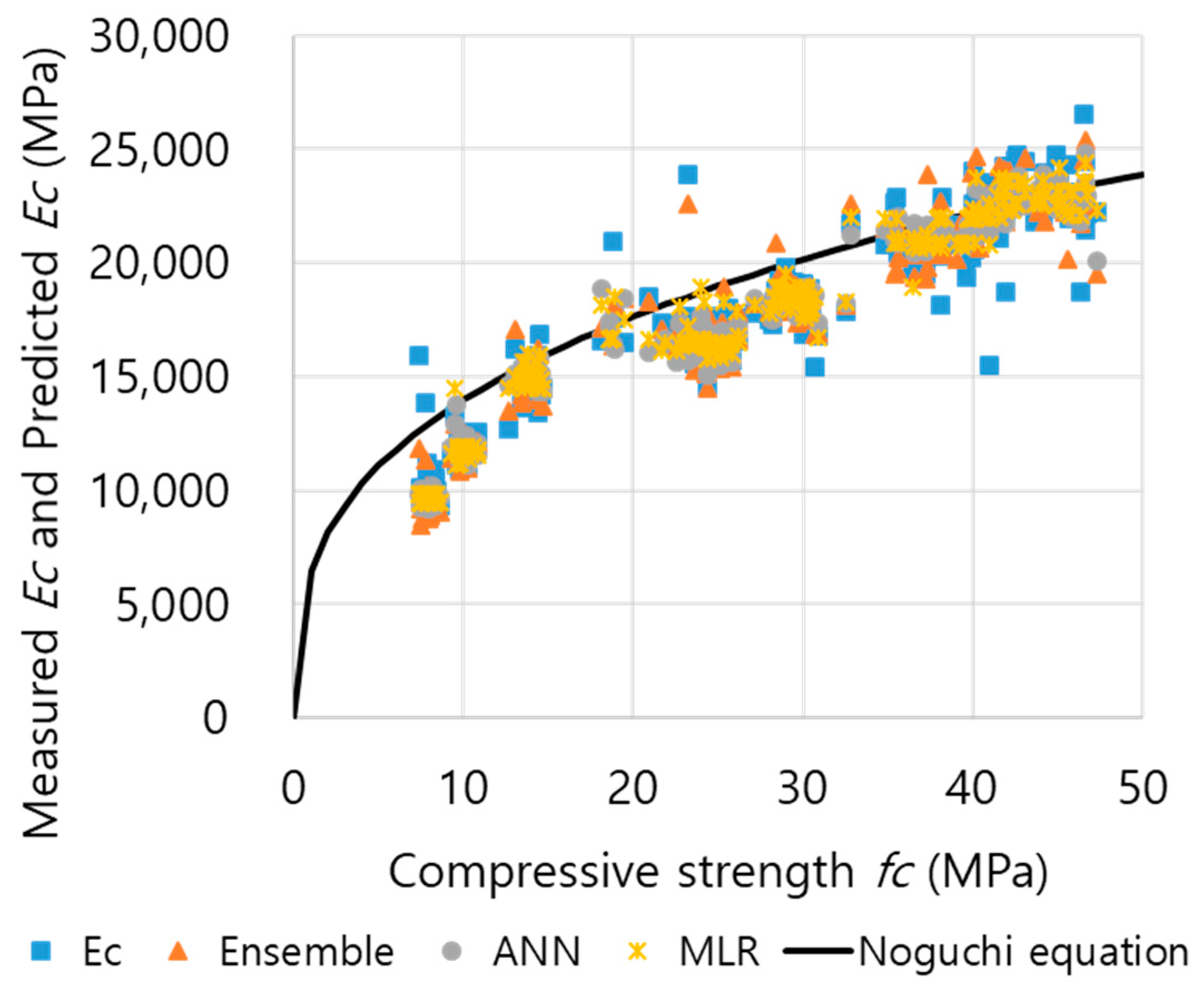
4.6. Relationship between Initial Chord and Compressive Strength

In the concrete cylinder in this study, materials similar to crushed cobblestone and granulated blast furnace slag (GBFS) were used, and Equation (17) (proposed by Noguchi) was used for comparison with the theoretical strength curve; k1 is the aggregate, and k2 is the correction coefficient of the SCMs [35]. According to

Table 13. Practical values of correction factor k1 and k2.

Lithological Type of Coarse Aggregate	k1	Type of Addition	k2
Crushed limestone, calcined bauxite	1.20	Silica fume, ground-granulated blast-furnace slag, fly ash fume	0.95
Crushed quartzitic aggregate, crushed andesite, crushed basalt, crushed clay slate, crushed cobblestone	0.95	Fly ash	1.10
Coarse aggregate, other than above	1.00	Addition other than above	1.00

, 0.95 for both k1 and k2 was used. Such concrete has the advantage of slow strength development at an early age but demonstrates significant progress for long-term strength.

$$E_c=k_1{k}_{2}33500{(f_c/60)}^{1/3}{({\omega }_c/2400)}^2\left(\mathrm{MPa}\right)$$

(17)

Figure 16 shows the relationship between the static elastic modulus (Ec) (Ec predicted from Ei, actual Ec) and compressive strength (fc). The theoretical strength curve of the Noguchi equation and trend of the measured Ec and fc data are suitable, and close to the line. Therefore, the Ec and fc are well-measured, and the values of Ec and fc are within a reasonable range. The results were the same for the Ec values predicted using the initial chord elastic modulus (Ei). Thus, it was confirmed that there is a high correlation (with intensity) when predicting the correct Ec using the Ei.

In this study, to confirm the accurate prediction and applicability of actual initial chord elastic modulus (Ei) values, the Ei was compared with the dynamic elastic modulus (Ed) of three theoretical equations, using a resonance frequency test. In addition, the relationship among the predicted Ei and static elastic modulus (Ec) values and the compressive strength (fc) was analyzed. It was found that the Ei is more correlated with the Ec than the Ed, confirming the need for accurate Ei prediction. In addition, it was confirmed that the correlation between the frequencies collected by the resonance frequency test according to the ASTM method (but not the fracture test) and the Ei and Ec was high, and that the Ei and Ec could be predicted using the resonance frequency. As a result of predicting the Ei using ML (ensemble, ANN), multiple linear regression (MLR), and correction factor methods from the collected frequency, it was possible to overcome the nonlinear behavior of concrete in the range of the initial Ec. Thus, the prediction error was smaller than when using the MLR or correction factor methods. The predicted Ei showed a higher correlation with the Ec and fc than the Ed and was able to identify the applicability of the Ei.

5. Conclusions

Predicting the static elastic modulus (Ec) is important for concrete structures. The ASTM resonance frequency test is commonly used in predicting a consistent dynamic elastic modulus (Ed) using a nondestructive method. The resonance frequency test calculates the Ed for a very small stress in the stress–strain curve and assumes that the Ed is equal to the initial chord elastic modulus (Ei). However, the calculated Ed derives a large error for utilizing the Ec and fc, owing to the nonlinearity of the concrete. Therefore, the correct Ei as extracted through the curve fitting of the stress-strain curve showed a better correlation between the Ec and fc than the Ed. These results indicate that it is desirable to measure and utilize accurate Ei values. In this study, it was possible to predict the actual Ei quite accurately by applying the ensemble, ANN, MLR, and correction factor methods to the f1 to f4 frequencies of longitudinal (LT) and transverse (TR) modes collected by the ASTM resonance frequency test. If several frequency variables were used, the contributions of the variables were extracted, and the relationships with the Ec and fc were analyzed using the predicted Ei. The following conclusions were drawn.

• The Ed values calculated by three theoretical equations (ASTM, Rayleigh Ritz) of the resonance frequency test were in the order of f1,f2.LT > ASTM.LT > ASTM.TR, and had nearly the same values. The size of the elastic modulus as measured by static and dynamic tests was Ed > Ei > Ec. In addition, it is determined that it is desirable to utilize the Ei, as the correlation with Ec is analyzed as Ei > Ed.
• The Popovis equation for the relationship between Ec and Ed gives results similar to the Eds of the ASTM, and the Lydon and Balendran equations are similar to Ei values. BS8110 Part 2 is not suitable, as because it has a large error from the Ed and Ei in the resonance frequency test.
• As a result of comparing an E-modulus based on ASTM.LT, f1,f2.LT, and ASTM.TR had a clear linear relationship, and they were close in the line of equality. They were identified as having a nonlinear relationship with the Ei and Ec. As the theoretical equations assumed the concrete as a perfectly elastic body for microscopic stress, it was difficult to overcome the nonlinear behavior of the actual Ei and Ec, owing to challenges in considering inhomogeneity and inelasticity of concrete. Thus, it is more appropriate to accurately predict and utilize the Ei, which has a similar nonlinear behavior with the Ec.
• As a result of applying ASTM.LT, f1,f2.LT, and ASTM.TR to the correction factors, the MAPE in the Ei could be lowered to 6.40%, 6.50%, and 6.43%, respectively. In addition, the Ed in the three equations and Ei of the MAPE decreased in order in days 4, 7, 14, and 28. The theoretical equation is suitable for concrete after 28 days but is considered difficult to use to accurately predict lower ages.
• In the relationship between Ei and frequency, the correlation of Ei-f1 was the largest, the nonlinearity increased as the mode appeared later, and the density and consistency of the data gradually decreased. In addition, the Ei and Ec values and first frequency of the resonance frequency test tended to be similar to an exponential function, indicating that prediction of the Ei and Ec based on frequency was possible.
• As a result of predicting the Ei using only frequencies through the ensemble and ANN methods, the MAPE decreased by 3.90% in the case of using only f1, and by 3.51% in the case of using f1-f4. Accordingly, the nonlinear behavior could be overcome by using ML.
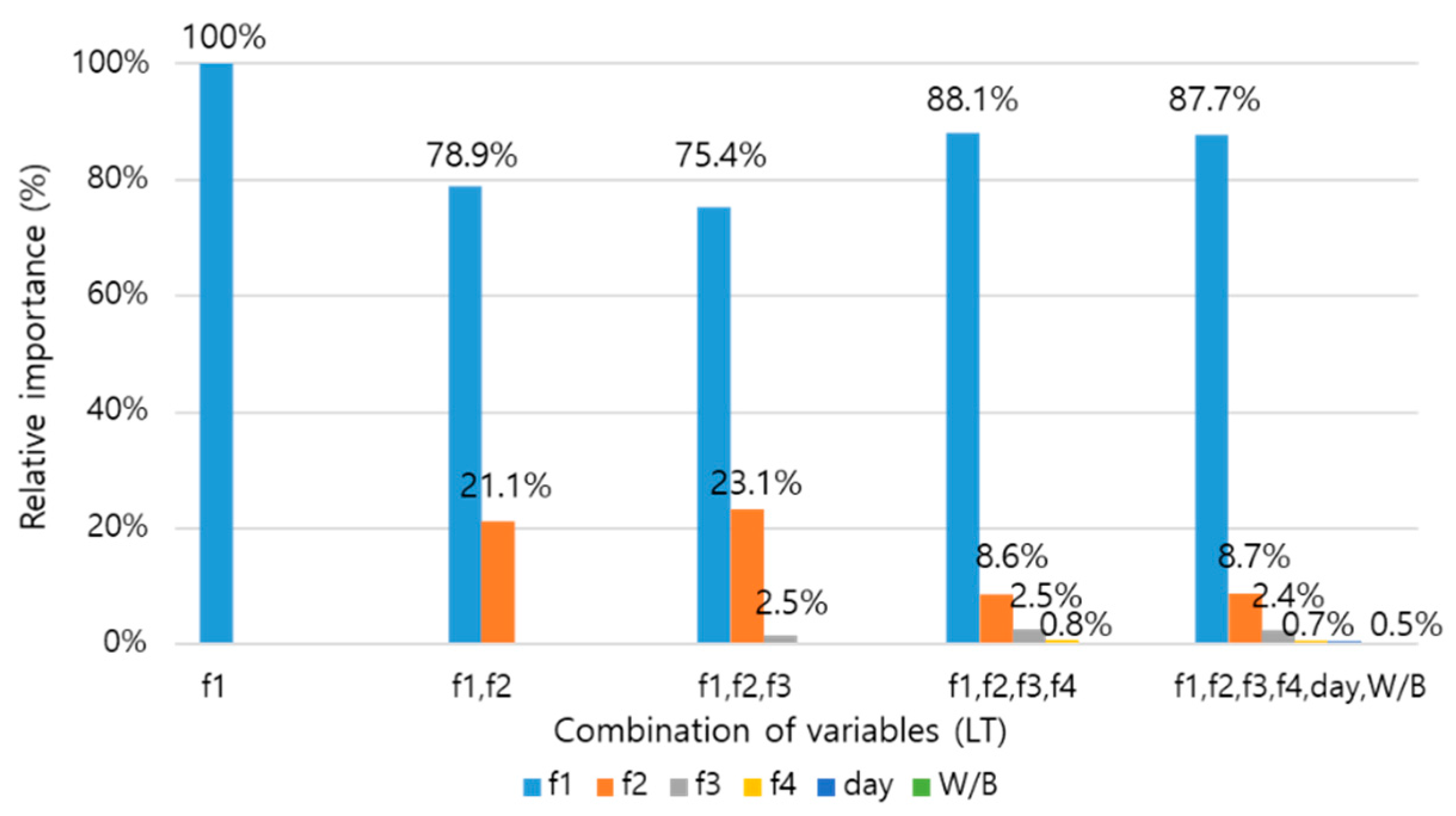
• As a result of analyzing the contributions of variables in predicting the Ei, f1 and f2 were dominant, the RI of the size factor was 0, and 0.3% of the day variables contributed to the Ei prediction. Therefore, it is possible to predict a sufficiently accurate Ei using only the frequencies, i.e., without other variables.
• As a result of predicting the Ec by applying a correction factor of 0.89 to the predicted Ei in four ways, the MAPE ranged from 4.6% to 6.57%, and the correlation between the predicted Ec and fc was high. Therefore, far more accurate Ei values can be predicted by the ASTM method in the future, and more accurate design, construction, and maintenance will be possible if this approach is used for calculating the Ec and fc.

References

1. Mehta, P.K.; Monteiro, P.J.M. Concrete-Microstructure, Properties, and Materials, 4th ed.; McGraw-Hill Education: New York, NY, USA, 2013. [Google Scholar]
2. ASTM Standard C666/C666M-15. Standard Test Method for Resistance of Concrete to Rapid Freezing and Thawing; ASTM International: West Conshohoken, PA, USA, 2015. [Google Scholar]
3. ASTM Standard C469/C469M-14. Standard Test Method for Static Modulus of Elasticity and Poisson’s Ratio of Concrete in Compression; ASTM International: West Conshohoken, PA, USA, 2014. [Google Scholar]
4. Popovics, J.S. A Study of Static and Dynamic Modulus of Elasticity of Concrete; ACI-CRC Final Report; American Concrete Institute: Farmington Hills, MI, USA, 2008. [Google Scholar]
5. ASTM Standard C597M-16. Standard Test Method for Pulse Velocity through Concrete; ASTM International: West Conshohoken, PA, USA, 2016. [Google Scholar]
6. ASTM Standard C215-14. Standard Test Method for Fundamental Transverse, Longitudinal, and Torsional Resonant Frequencies of Concrete Specimens; ASTM International: West Conshohoken, PA, USA, 2016. [Google Scholar]
7. Lee, B.J.; Kee, S.-H.; Oh, T.K.; Kim, Y.Y. Effect of Cylinder Size on the Modulus of Elasticity and Compressive Strength of Concrete from Static and Dynamic Tests. Adv. Mater. Sci. Eng. 2015, 2015, 1–12. [Google Scholar] [CrossRef] [Green Version]
8. Park, J.Y.; Yoon, Y.G.; Oh, T.K. Prediction of Concrete Strength with P-, S-, R-Wave Velocities by Support Vector Machine (SVM) and Artificial Neural Network (ANN). Appl. Sci. 2019, 9, 4053. [Google Scholar] [CrossRef] [Green Version]
9. Lee, B.J.; Kee, S.-H.; Oh, T.; Kim, Y.-Y. Evaluating the Dynamic Elastic Modulus of Concrete Using Shear-Wave Velocity Measurements. Adv. Mater. Sci. Eng. 2017, 2017, 1–13. [Google Scholar] [CrossRef] [Green Version]
10. Jurowski, K.; Grzeszczyk, S. Influence of Selected Factors on the Relationship between the Dynamic Elastic Modulus and Compressive Strength of Concrete. Materials 2018, 11, 477. [Google Scholar] [CrossRef] [Green Version]
11. Kolluru, S.V.; Popovics, J.S.; Shah, S.P. Determining Elastic Properties of Concrete Using Vibrational Resonance Frequencies of Standard Test Cylinders. Cem. Concr. Aggreg. 2000, 22, 81–89. [Google Scholar] [CrossRef]
12. Popovics, S. Verification of relationships between mechanical properties of concrete-like materials. Mater. Struct. 1975, 8, 183–191. [Google Scholar] [CrossRef]
13. British Standard Institute. Structural Use of Concrete—Part 2: Code of Practice for Special Circumstance; BS 8110-2:1995; BSI: London, UK, 1985. [Google Scholar]
14. Lydon, F.D.; Balendran, R.V. Some observations on elastic properties of plain concrete. Cem. Concr. Res. 1986, 16, 314–324. [Google Scholar] [CrossRef]
15. Diogenes, H.J.F.; Cossolino, L.C.; Pereira, A.H.A.; Eldebs, M.K.; Eldebs, A.L.H.C. Determination of modulus of elasticity of concrete from the acoustic response. IBRACON Struct. Mater. J. 2011, 4, 803–813. [Google Scholar]
16. Aguilar, R.; Ramirez, E.; Hacch, V.G.; Pando, M.A. Vibration-based nondestructive testing as a practical tool for rapid concrete quality control. Constr. Build. Mater. 2016, 104, 181–190. [Google Scholar] [CrossRef]
17. Shih, Y.F.; Wang, Y.R.; Lin, K.L.; Chen, C.W. Improving non-destructive concrete strength tests using support vector machines. Materials 2015, 8, 7169–7178. [Google Scholar] [CrossRef]
18. Chopra, P.; Sharma, R.K.; Kumar, M. Prediction of compressive strength of concrete using artificial neural network and genetic programming. Adv. Mater. Sci. Eng. 2016, 2016, 1–10. [Google Scholar] [CrossRef] [Green Version]
19. Chithra, S.; Kumar, S.S.; Chinnaraju, K.; Ashmita, F.A. A comparative study on the compressive strength prediction models for high performance concrete containing nano silica and copper slag using regression analysis and artificial neural networks. Constr. Build. Mater. 2016, 114, 528–535. [Google Scholar] [CrossRef]
20. Han, I.J.; Yuan, T.F.; Lee, J.Y.; Yoon, Y.S.; Kim, J.H. Learned Prediction of Compressive Strength of GGBFS Concrete Using Hybrid Artificial Neural Network Models. Materials 2019, 12, 3708. [Google Scholar] [CrossRef] [PubMed] [Green Version]
21. Erdal, H.I.; Karakurt, O.; Namli, E. High performance concrete compressive strength forecasting using ensemble models based on discrete wavelet transform. Eng. Appl. Artif. Intell. 2013, 26, 1246–1254. [Google Scholar] [CrossRef]
22. Yan, K.; Shi, C. Prediction of elastic modulus of normal and high strength concrete by support vector machine. Constr. Build. Mater. 2010, 24, 1479–1485. [Google Scholar] [CrossRef]
23. Young, B.A.; Hall, A.; Pilon, L.; Gupta, P.; Sant, G. Can the compressive strength of concrete be estimated from knowledge of the mixture proportions?: New insights from statistical analysis and machine learning methods. Cem. Concr. Res. 2019, 115, 379–388. [Google Scholar] [CrossRef]
24. Cihan, M.T. Prediction of Concrete Compressive Strength and Slump by Machine Learning Methods. Adv. Civ. Eng. 2019, 2019, 1–11. [Google Scholar] [CrossRef]
25. ASTM Standard C31/C31M-12. Standard Practice for Making and Curing Concrete Test Specimen in the Field; ASTM International: West Conshohoken, PA, USA, 2012. [Google Scholar]
26. ASTM Standard C39/C39M-14a. Standard Test Method for Compressive Strength of Cylindrical Concrete Specimens; ASTM International: West Conshohoken, PA, USA, 2014. [Google Scholar]
27. Carreora, D.J.; Cju, K.H. Stress-strain relationship for plain concrete in compression. ACI J. 1985, 82, 797–804. [Google Scholar]
28. Hognestad, E. A Study on Combined Bending and Axial Load in Reinforced Concrete Members; Report: University of Illinois Engineering Experiment Station, No. 399; University of Illinois: Champaign, IL, USA, 1951. [Google Scholar]
29. Benkaddour, M.K.; Bounoua, A. Feature extraction and classification using deep convolutional neural networks, PCA and SVC for face recognition. Trait. Signal 2017, 34, 77–91. [Google Scholar] [CrossRef]
30. Hansen, L.K.; Salamon, P. Neural network ensembles. IEEE Trans. Pattern Anal. Mach. Intell. 1990, 12, 993–1001. [Google Scholar] [CrossRef] [Green Version]
31. Rosenblatt, F. Principles of Neuro Dynamics: Perceptrons and the Theory of Brain Mechanisms; Spartan Books: Washington, DC, USA, 1962; pp. 29–51. [Google Scholar]
32. Rumerlhar, D.E. Learning representation by back-propagating errors. Nature 1986, 323, 533–536. [Google Scholar]
33. Daliakopoulos, I.N.; Coulibaly, P.; Tsanis, I.K. Groundwater level forecasting using artificial neural networks. J. Hydrol. 2005, 309, 229–240. [Google Scholar] [CrossRef]
34. Barnett, V.; Lewis, T. Outliers in Statistical Data, 3rd ed.; John Wiley & Sons: New York, NY, USA, 1994. [Google Scholar]
35. Noguchi, T.; Tomosawa, F.; Nemati, K.M.; Chiaia, B.M.; Fantilli, A.P. A practical equation for elastic modulus of concrete. ACI Struct. J. 2009, 106, 690–696. [Google Scholar]
Figure 1. Experimental setup for static destructive test.
Applsci 10 05464 g001
Figure 2. Resonance frequency test setup. (a) longitudinal mode and (b) transverse mode.
Applsci 10 05464 g002
Figure 3. Resonance frequency by curing ages according to ASTM resonance test. (a) frequencies of longitudinal mode, (b) frequencies of transverse mode.
Applsci 10 05464 g003
Figure 4. Extraction of initial chord elastic modulus (Ei) from stress-strain curve.
Applsci 10 05464 g004
Figure 5. Procedure of ensemble from an input sample.
Applsci 10 05464 g005
Figure 6. Procedure of artificial neural network from an input sample.
Applsci 10 05464 g006
Figure 7. Comparison of static elastic modulus (Ec), Ei, and dynamic elastic modulus (Ed).
Applsci 10 05464 g007
Figure 8. Comparison of Ed and Ei by ages and mixes according to ASTM.LT. (a) Mix 1 (20 MPa), (b) Mix 2 (40 MPa).
Applsci 10 05464 g008
Figure 9. Comparison of first frequency of LT mode and E-modulus.
Applsci 10 05464 g009
Figure 10. Relationship between the frequencies and Ei of the resonance frequency test. (a) LT frequencies-Ei, (b) TR frequencies-Ei.
Applsci 10 05464 g010
Figure 11. Comparison of prediction results with two frequencies. (a) Predicted Ei with multiple linear regression (MLR), (b) Predicted Ed with Equation (4).
Applsci 10 05464 g011
Figure 12. Relative importance according to combination of variables in LT mode.
Applsci 10 05464 g012
Figure 13. Relative importance according to combination of variables in TR mode.
Applsci 10 05464 g013
Figure 14. Comparison of Ei predicted with machine learning (ML) and actual Ei. (a) Ei predicted by frequency of LT mode, (b) Ei predicted by frequency of TR mode.
Applsci 10 05464 g014
Figure 15. Comparison of Ec predicted with Ei and actual Ec.
Applsci 10 05464 g015
Figure 16. Relationship between Ec (measured Ec and predicted Ec) and fc.
Applsci 10 05464 g016