Induction Motor Fault Classification Based on FCBF-PSO Feature Selection Method

Abstract

This study proposes a fast correlation-based filter with particle-swarm optimization method. In FCBF–PSO, the weights of the features selected by the fast correlation-based filter are optimized and combined with backpropagation neural network as a classifier to identify the faults of induction motors. Three significant parts were applied to support the FCBF–PSO. First, Hilbert–Huang transforms were used to analyze the current signals of motor normal, bearing damage, broken rotor bars and short circuits in stator windings. Second, ReliefF, symmetrical uncertainty and FCBF three feature-selection methods were applied to select the important features after the feature was captured. Moreover, the accuracy comparison was performed. Third, particle-swarm optimization (PSO) was combined to optimize the selected feature weights which were used to obtain the best solution. The results showed excellent performance of the FCBF–PSO for the induction motor fault classification such as had fewer feature numbers and better identification ability. In addition, the analyzed of the induction motor fault in this study was applied with the different operating environments, namely, SNR = 40 dB, SNR = 30 dB and SNR = 20 dB. The FCBF–PSO proposed by this research could also get the higher accuracy than typical feature-selection methods of ReliefF, SU and FCBF.

1. Introduction

Nowadays, automated production has become a trend. The number of unmanned factories is increasing, which means that the stability requirements of machinery and equipment are also increasing. Therefore, failure analysis of the motor and how to determine the type of failure has become an important subject. In general, motor failures are divided into two categories: electrical and mechanical failures. Most mechanical damage occurs in stators, rotors and bearings. Among them, bearing failure is the most common as shown in

Table 1. Proportion of motor failure types.

Failure Type	Occurrence Percentage
Bearing damage	45%
Stator damage	35%
Rotor damage	10%
Others damage	10%

[1].

In this research, the current signal amount was measured and analyzed under different motor conditions. Current signal was selected for measurement because it was less affected by vibration and temperature signals. It also could be used for online monitoring to understand the motor operating status in real time. There are several studies focusing on data analysis methods, such as fast Fourier transform (FFT), wavelet transform (WT) and Hilbert–Huang transform (HHT). However, data of FFT need periodicity and selection of wavelet functions is difficult for wavelet multianalysis [2,3]. The HHT use empirical mode decomposition (EMD) to decompose the signal and allow intrinsic mode functions (IMF) to hold unique frequency information that can capture more useful features.

In recent years, measurement signals have been converted by analysis methods and classified by algorithms such as artificial neural network (ANN) [4], probability neural network (PNN) [5,6] and backpropagation neural network (BPNN) [7,8]. These have been frequently used in different fields. For the BPNN, its neurons are set in advance. The number of the neurons and the learning rate are extremely important. The gradient method is used to find the best solution. Therefore, this research uses BPNN for discussion.

In [9], Yu, Lei and Liu, Huan proposed a fast correlation-based filter (FCBF) feature-selection method that uses symmetric uncertainty (SU)—instead information gain (IG)—to determine the correlation between features and categories, or whether there is redundancy between the features. This study was done through the calculation of the SU value between features and categories, features and features, and compared with the results of ReliefF feature selection proposed by Kononeill in 1994. The FCBF is one of the feature-weighting algorithms [10] to address complex and multi-category situations. The comparison results show that the FCBF method is faster than other methods and obtains corresponding classification results. Furthermore, if a higher correlation threshold is set, the efficiency of the FCBF can be further improved. In addition, the FCBF method can obtain a better classifier recognition result by changing the feature selection order [11].

In this study, particle-swarm optimization (PSO) is applied to optimize the weights of important features after screening. Inspired by the observation of swarming bird behavior during foraging, it is used to find the best solution to improve the accuracy (Acc) of the classifier. The PSO is a group-based optimization search technology, similar to a genetic algorithm (GA) [12]. PSO and GA have ability to randomly initialize, and both use adaptive values for random search. However, although there is no guarantee that the best solution can be found, for PSO, it has memory.

2. Signal Analysis and Neural Network

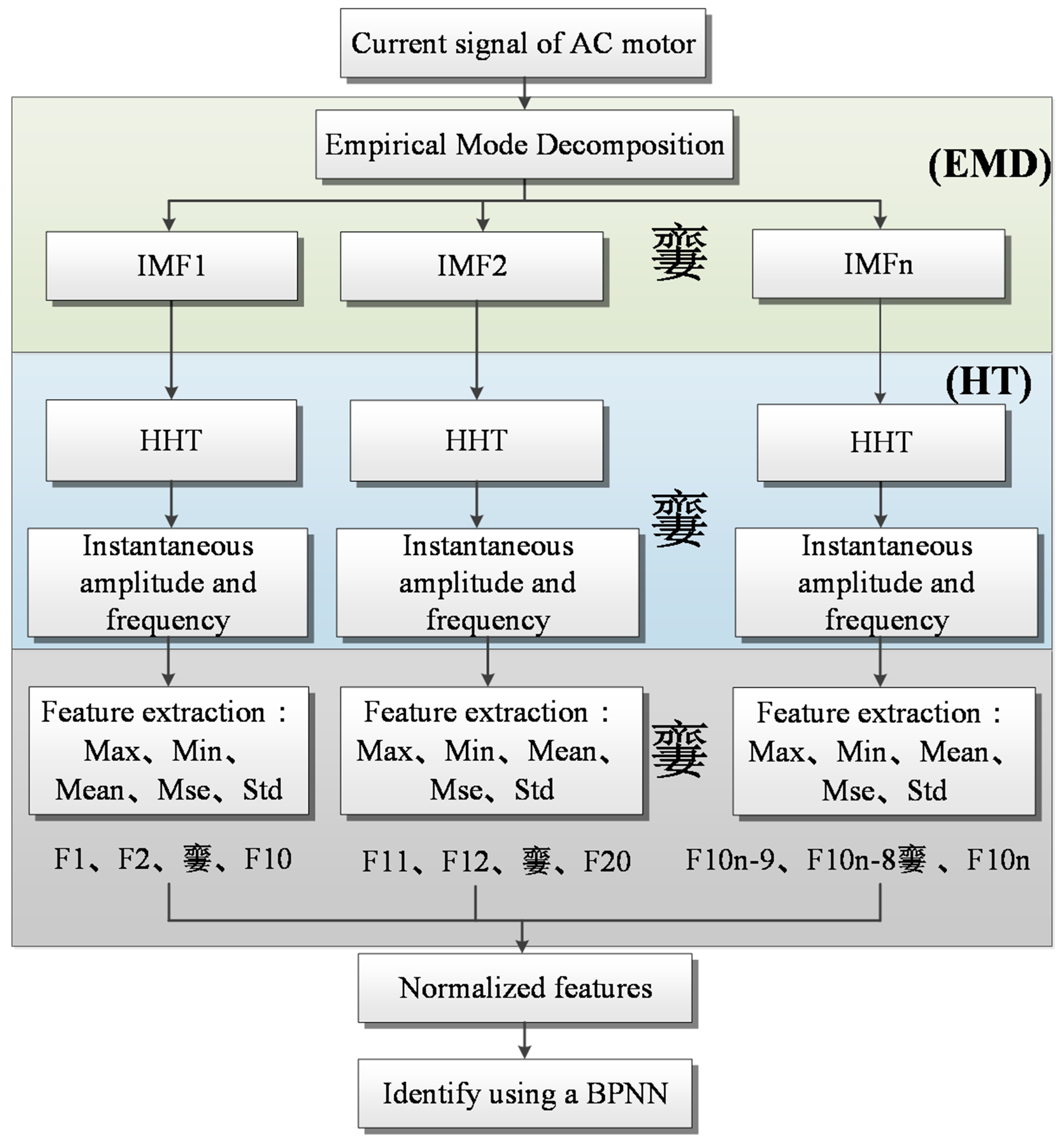
2.1. Hilbert–Huang Transform (HHT)

According to the mathematical theory of modern well-known mathematician Hilbert, HHT proposed by Norden E. Huang in 1998 [13]. The original signal is decomposed into IMF by EMD [14,15] to obtain the instantaneous frequency of the analysis data. HHT conversion has a good analysis effect on the analysis of nonstable or nonlinear signals.

2.1.1. Intrinsic Mode Functions

For any function, if the following two conditions are met, it can be called the IMF:

• The sum of the number of local maximum and local minima must be the same as or different from the number of zero-crossings, which means that an extreme value must have a zero-crossing point behind it.
• At any time, the upper envelope defined by the local maximum and the lower envelope defined by the local minimum must be averaged to approach zero.

2.1.2. Empirical Mode Decomposition

EMD is the signal processing before HHT, which decomposes the signal into a combination of IMF. Due to the HHT’s restrictions on the instantaneous frequency, if the general signal data are directly used, the complete and correct instantaneous frequency cannot be obtained. The steps of EMD screening IMF are listed as follows:

Step 1.

Input the original signal $x(t)$ to find the local maximum and local minima. Connect their values to upper envelope $H(t)$ and lower envelope $L(t),$ respectively;

Step 2.

Calculate the average of the upper envelope $H(t)$ and the lower envelope $L(t)$ to get the mean envelope $m(t)$;

Step 3.

Subtract the original signal $x(t)$ from the mean line $m(t)$ to get $h(t)$;

Step 4.

Check whether $h(t)$ meets the conditions of the IMF. If not, go back to Step 1 and replace $x(t)$ with $h(t)$. Rescreen until $h(t)$ meets the conditions and termination of IMF, and store $h(t)$ as the component $C_i$ of IMF;

Step 5.

Subtract the $h(t)$ from original signal$x(t)$ to get $R(t)$;

Step 6.

Check whether $R(t)$ is monotonic function or not. If yes, stop decomposition. If not, repeat Step 1 to Step 5.

Therefore, the original data can be decomposed into n IMFs and a trend function, and we can perform HHT on the IMF for signal analysis. The flowchart of the EMD is shown in Figure 1.

2.2. Hilbert Transform (HT)

The Hilbert transform (HT) method changes the previous analysis of nonlinear and nonsteady state. For the combination of IMF, HT is used to obtain the instantaneous amplitude and instantaneous frequency between signals.

Through the equation, the instantaneous amplitude $a_i(t)$ and instantaneous phase angle ${\varphi }_i(t)$ can be obtained, which can be converted into (1) and (2). By differentiating the time with the instantaneous phase ${\varphi }_i(t)$, the instantaneous frequency ${\mathsf{\omega }}_i(t)$ can be obtained, as shown in (3).

$$a_i(t)=\sqrt{C_i{}^2(t)+H_i{}^2(t)}$$

(1)

$${\varphi }_i(t)=arctan\left[\frac{H_i(t)}{C_i(t)}\right]$$

(2)

$${\omega }_i(t)=\frac{d{\varphi }_i(t)}{dt}$$

(3)

Then, through these calculations, the distribution including frequency, time, and energy can be obtained using the instantaneous amplitude $a_i(t)$ and the instantaneous frequency ${\mathsf{\omega }}_i(t)$. This result is called the Hilbert spectrum.

2.3. Neural Network (NN)

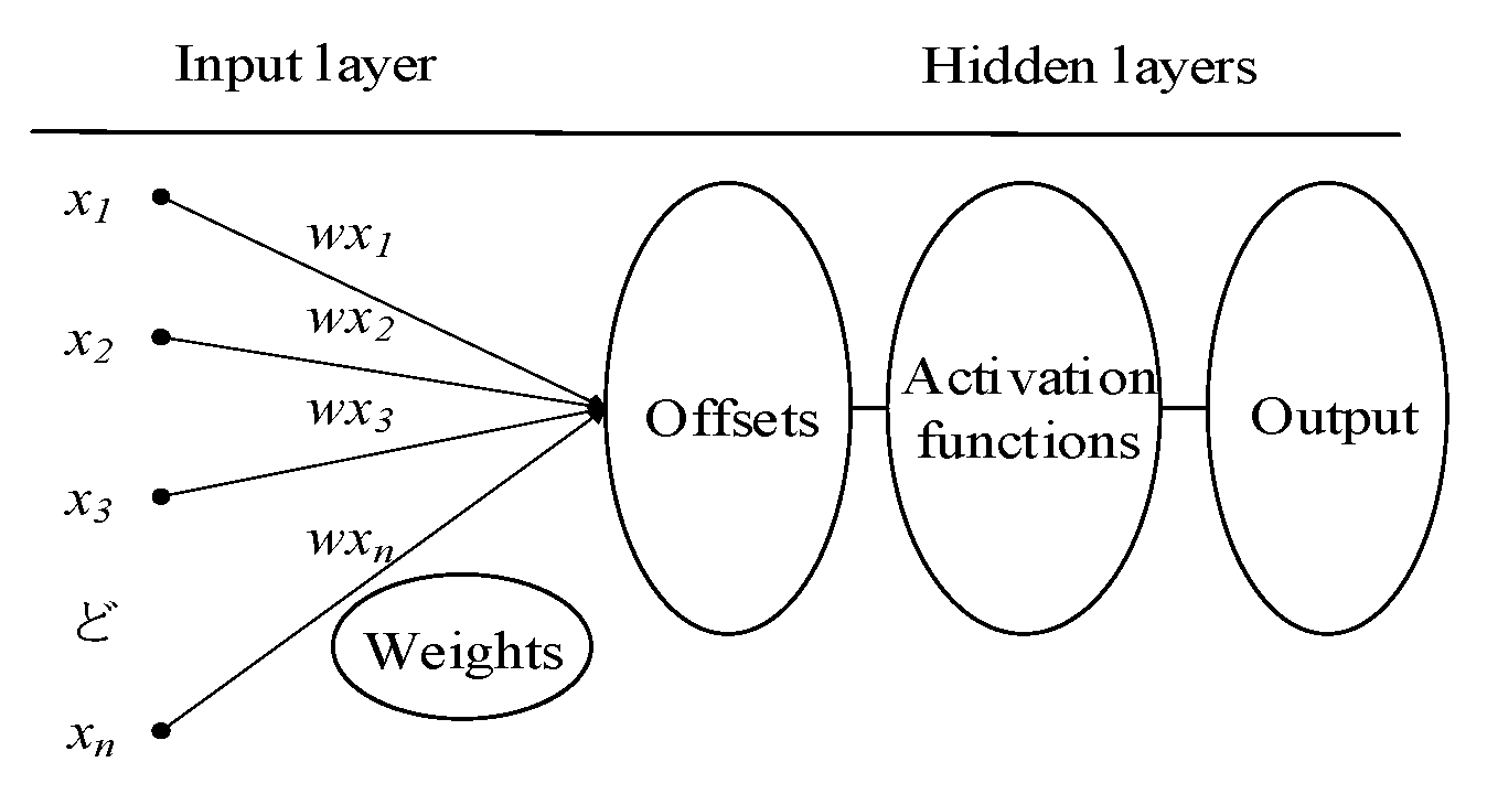
2.3.1. Architecture of NN

Neural network (NN) was proposed by Mcculloch and Pitts in 1943. According to the information processing method established by the biologic nervous system, the network structure is constructed by several neurons. Through the interconnection of many neurons, the information transmitted from the outside world is processed and memorized, so that the corresponding response to the resulting changes can be facilitated. This includes an input layer, n hidden layers and an output layer.

2.3.2. Back Propagation Neural Network (BPNN)

The neural network (NN) is an operational model, consisting of interconnected neurons. Each node represents a specific output function, called the activation function [16]. Each connection between two neurons represents a weight. In the initial stage, the weights and offsets of NN are fixed and there is no learning ability. In 1986, the BPNN feedforward neural network model was proposed by Rumelhart et al. [17]. The network refers to the hierarchy of neurons. It consists of input layers, hidden layers and output layers. As shown in Figure 2, this research used the neural network toolbox (NNTOOL) in Matlab to create and train cascaded artificial neural networks. In the experiment, a three-layer feedforward neural network is trained by using the scaled conjugate gradient (SCG) algorithm. The activation function at the hidden layer is a hyperbolic tangent sigmoid transfer function and output layers are log-sigmoid transfer functions in the network. The numbers of hidden neurons applied in the verification are 10. As long as its weight, net-input and transfer function have derivative functions, the network can be trained. Moreover, the reason to choose SCG is that it is based on supervised learning and is comparatively faster than the standard backpropagation model [18].

3. Feature-Selection Method and Application

To achieve the best performance of the algorithm, the choice of features can be regarded as an extremely important method. Including in feature selection are feature extraction and feature construction. Among them, Yu and Liu [9] classified the feature subsets into four categories: (a) completely irrelevant and noisy features, (b) weakly relevant and redundant features, (c) weakly relevant and nonredundant features and (d) strongly relevant features. An optimal subset mostly contains all the features in the category (c) and (d) as shown in Figure 3. In addition, feature selection involves two main objectives, which are to maximize the classification accuracy and minimize the number of features [19]. Strongly relevant features are indispensable for the enhancement of discriminative power and prediction accuracy. Sometimes, weakly relevant features can be useful for improving prediction accuracy if a feature is nonredundant and compatible with evaluation measures [20]. Moreover, the curse of dimensionality of data poses a severe challenge to many existing feature-selection methods with respect to efficiency and effectiveness [21,22]. The results of this research also compared various feature selection methods to highlight the efficiency and effectiveness of FCBF [23,24]. In summary, the main purpose of FCBF–PSO proposed in this study is to quickly screen out important features and improve accuracy.

3.1. ReliefF

ReliefF is a feature-weighting algorithm proposed by Kira in 1992. Because it is limited to the classification of two kinds of data, it has not been applied too much. Hence, Kononeill expanded it in 1994. ReliefF feature selection is proposed to deal with more complex multi-category situations [25]. This method is simple and relatively efficient in execution. This feature-selection method uses correlations between the calculation characteristics and each fault category by randomly selecting any sample $Y_m$ from its training sample set and through the sample set of the same category as $Y_m$, taking K of the same category as $Y_m$. The neighboring sample H can be called near-hits. Similarly, find k-nearest neighbor samples M from the sample set and which are different from the $Y_m$ category, which can be called near-misses. This study sorts the weights of the features from high into low to facilitate the research. However, a limitation of this algorithm is that it cannot effectively remove redundant features. the steps of ReliefF are listed as follows:

Step 1.

Set feature set $F=\{F_1{,F}_2{\dots \dots ,F}_N$}, sample category, $Y=\left\{Y_1{,Y}_2{\dots \dots ,Y}_N\right\}$, sampling times Z, the number of neighbor samples K, the threshold r of feature weights and the initial weight of each feature are zero;

Step 2.

Randomly select any sample $Y_m$ from all the sample types of Y;

Step 3.

Extract K adjacent samples of the same category as the sample $Y_m$;

Step 4.

K Near-misses are also found from the sample set sums different from the $Y_m$ category;

Step 5.

Calculate the weight of each feature in (4);

Step 6.

Repeat sampling to determine whether the number of sampling times Z was reached. If not, return to Step 2 and repeat until the maximum number of sampling times is reached;

Step 7.

Sorting features according to feature weights from large to small is mean the importance of the selected features;

Step 8.

Calculate the sum of the feature weights of the first n items (expressed as W_all)

Step 9.

If W_all < r then n + 1 and repeat Step 8 until W_all > r stops, where r is 90% of the sum of all feature weights;

Step 10.

Output the feature.

$$\begin{array}{c}W(N)=W(N)-{\displaystyle \sum _{j=1}^K\frac{diff(N,Y,H_j)}{ZK}}\\ +{\displaystyle \sum {}_{C\notin class}(Y)}\left[\frac{p(C)}{1-p(class(R))}{\displaystyle \sum _{j=1}^{K}diff(N,Y,H_j(C))}\right]\\ /(ZK)\end{array}$$

(4)

Among them, N is the number of features, K is the nearest neighbor sample taken by samples of different categories, Y is the sample category, Z is the number of samplings and k-nearest neighbors $H_j(j=1,2,\dots K)$ in the same sample set of $Y_m$ can be found, $y_1$ and $y_2$ in ${diff(N,y}_1{,y}_2)$ can expressed as the difference from feature N.

3.2. Symmetrical Uncertainty (SU)

3.2.1. Information Entropy

Information entropy is the average amount of information contained in a message, which was proposed by Shannon in 1948 [26]. Among them, entropy is generally understood as a measure of uncertainty rather than certainty. Because the more random the message, the greater the entropy value, which also explains the probability distribution of the sample in information theory. The reason for using the logarithm of probability distribution as the information measure is that it is additive. The formula for entropy is shown in (5). Moreover, the information gain is shown in (6).

$$H(t)=-k{\displaystyle \sum _i^{N}P(x_i)}I(x_i)$$

(5)

$$I(X)={\displaystyle \sum _i^N\ln P(x_i)}$$

(6)

Among them, P is the probability mass function of x, k is a proportional constant corresponding to the selected metric, and i is the information body of x.

3.2.2. Symmetrical Uncertainty Method

For variables, the correlation and degree of influence between them is usually the most direct and fastest method of judgment. By calculating the correlation coefficient, it is usually possible to quickly obtain the correlation between the two, but if the correlation is used to select features, it usually results in a tendency to select features with larger values. Therefore, this research uses the method of SU to calculate the correlation between features and targets [27]. Calculation of SU is shown in (7).

$$SU(X,Y)=\frac{I(X)}{H(X)+H(Y)}$$

(7)

It can also be explained from the definition that it is a form of information gain normalization. Nonlinear related information variables defined based on information entropy, used to reconstruct the degree of correlation between nonlinear random variables. Among them, the symmetric uncertainty is calculated using the SU value, which effectively corrects the bias about the selected feature. After normalizing the information gain, the SU value is between 0 and 1. Make the two different types relatively fair when comparing and explain that when $SU(X,Y)=1$, it means that X and Y are completely related; otherwise, when $SU(X,Y)=0$, it can be judged that X and Y are completely independent individuals.

3.3. Fast Correlation-Based Filter (FCBF)

This research uses the FCBF feature-selection method, which was proposed in 2004. It uses the SU value to replace the information gain and performs the calculation of selection [28]. This method can be divided into two parts. First use the features to sort the SU value of the fault type and use the threshold setting to delete the less influential features. Then compare the features, as shown in Figure 4. Because the correlation between features $T_1$ and $T_2$, $T_4$ is higher than the relationship between $T_2$, $T_4$ and category, consider $T_2$, $T_4$ as redundant features with less correlation and delete them. The advantage of this method is that you can compare the correlation of features and perform feature selection at the same time and use features with higher correlation to filter other features that have not been deleted. In this way, the efficiency of calculation while filtering is achieved and the calculation is accelerated, and the recognition rate is improved.

The steps of the process of FCBF feature selection are as follows:

Step 1.

Set the data set $(x_i{,t}_i)$,${i=1,\dots \dots ,N\mathrm{and}x}_i{=[x}_{i1}{,x}_{i2}{,\dots \dots ,x}_{id}{]}^T\in R^n$,$t_i{=[t}_{i1}{,t}_{i2}{,\dots ,t}_{im}{]}^T\in R^m$. Sample category is ${Y=(y}_1{,y}_2{,\dots y}_N)$;

Step 2.

Calculate the SU value between each feature $t_i$ and category Y;

Step 3.

Store the $SU(t_i,Y)$ values of each feature and category in descending order into the S set;

Step 4.

Calculate the sum of SU in the first n items in the S set (expressed as $SU\_all$);

Step 5.

If $SU\_all<r$, then n+1 repeat to Step 4 until $S\_all$ > r stops, where r is 90% the sum of the S set;

Step 6.

Remove features after nth from S (Remove features with less influence);

Step 7.

Select the feature $T_1$ with the largest ${SU(t}_i,Y)$ value from S as the main feature for selecting;

Step 8.

Calculate the $SU(t_i{,T}_1)$ of other features and main features in order and the ${SU(t}_i,Y)$ values between this feature and category Y;

Step 9.

If ${SU(t}_i{,T}_1) \ge {SU(t}_i,Y)$, it is regarded as a redundant feature and deleted from S;

Step 10.

The main feature is stored in S’ and deleted from S;

Step 11.

Repeat Step 7 to Step 10 until S is the empty set and stop;

Step 12.

The output S’ is expressed as an important feature.

Among them, the process of FCBF feature screening is divided into two stages. First, the SU value is used to distinguish the features, and second, by comparing the correlation between the features and the features, to distinguish whether the features are redundant. The flowchart of this method is shown in Figure 5.

3.4. Application of FCBF–PSO

PSO is a type of macro-heuristic algorithm proposed by James Kennedy and Russell Eberhart in 1995. This algorithm was developed from bird watching and foraging behaviors. The principle is that multiple randomly distributed particles in space represent individuals in the bird population, and the position of each particle is assumed to be the best potential solution in the optimization problem. Since each particle is a feasible solution, the particle will have a fitness value after the operation. Based on the particle’s own experience and the group’s experience, the flight speed and direction are updated again and iteratively repeated to make all particles converge to the best solution. As shown in (8) and (9) [29]. Among them, this study combines the feature-selection method of FCBF to optimize the weight of the selected features. The acceleration factors $C_1$ and $C_2$ are linearly reduced from 2.5 to 0.5. The weight $\mathsf{\omega }$ is arbitrarily selected from 0.5 to 1 as in (10). Steps of FCBF–PSO is listed as follows:

$$\begin{array}{c}{V}_i(t+1)=\omega \times V_i(t)+C_1(t)r_1(t)(P_{best}-X_i)\\ +C_2(t)r_2(t)(G_{best}-X_i)\end{array}$$

(8)

$$X_i(t+1)=X_i(t)+V_i(t+1)$$

(9)

$$\omega =0.5+rand/2$$

(10)

Step 1.

Initially, in the d-dimensional space, parameters including particle number, number of iteration T, acceleration factors $C_1$, $C_2$ and its own weight $\mathsf{\omega }$ are set to form a particle population;

Step 2.

In space, assume that each feature is the coordinate of each particle $X_i{=(X}_{i1}{,X}_{i2}{,\dots \dots ,X}_{ij})$ and the flying speed of each particle is $V_i{=(V}_{i1}{,V}_{i2}{,\dots \dots ,V}_{ij})$;

Step 3.

Use FCBF feature-selection method to output important features $F_j$;

Step 4.

Bring the coordinates of the particles into the features $F_i{=(X}_{i1}{\times F}_1{,X}_{i2}{\times F}_2{,\dots \dots ,X}_{ij}{\times F}_j)$ to obtain the individual best solution $P_{best}$ and the group best solution $G_{best}$;

Step 5.

Use $P_{best}$ and $G_{best}$ to modify the particle’s flight speed $V_{i\_new}$ as shown in (10);

Step 6.

Correct the position $X_{i\_new}$ of the particle with the updated flight speed $V_{i\_new}$ to find a new position and speed;

Step 7.

If it meets the set number of iterations $T_{Max}$, it will stop, otherwise repeat Step 3 to Step 5, usually the termination condition is to reach the best solution or to reach the number of iterations set by yourself;

Step 8.

All particles converge to obtain the best solution;

Step 9.

Finally, after the optimization process, a set of solutions with the optimal particle coordinates $X_{best}$ can be obtained, which is the optimized feature weight.

Among them, the method of optimizing feature weights of FCBF–PSO retains the important features of FCBF feature-selection method and optimizes the weights. The flowchart of the method proposed by this institute is shown in Figure 6.

4. Experiment of Motor Failure and Measurement Signal Method

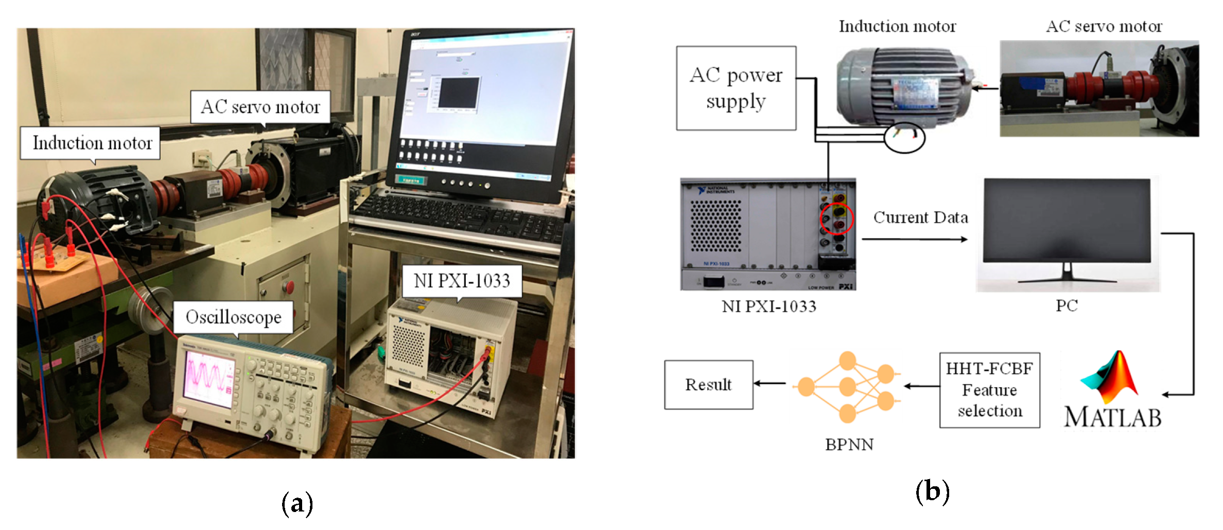
4.1. Experiment Apparatus

The equipment used in this experiment was a three-phase squirrel-cage induction motor. Its specifications are shown in

Table 2. Specifications of the induction motor.

Three-Phase Squirrel-Cage Induction Motor Specifications
Voltage	220 V/380 V	Output	2 HP 1.5 kW
Speed	1715 rpm	Current	5.58 A/3.23 A
Insulation	E	Poles	4
Effectiveness	83.5(100%)	Frequency	60 Hz

, and the types of induction motor failures used in this study are shown in Figure 7a–f. The power test platform is shown in Figure 7g, NI PXI-1033 signal acquisition device, digital electric meters and personal computers. The power test platform also includes servo motors, torque sensors and control panels. By using the above equipment, the measurement and analysis of the motor current signal could be completed.

4.2. Experiment Process

First, the flow of this study uses the servo motor of the power platform to be the load and is driven by the AC motor to made the motor run. Secondly, the motor current signal of any phase was captured for four different faulted through the signal picker, in which the sampling time of each data were 100 s, the acquisition frequency was 1000 Hz and 100 signals were measured for each signal. Finally, used the compiler analysis program MATLAB to HHT the measured signal on the computer and combine various feature screening methods. Using BPNN to compare its accuracy, the flow chart of its experimental architecture is shown in Figure 8a,b. We also repeated the calculation 200 times to obtain the average accuracy and performed the feature-selection method multiple times to ensure this study was repeatable and stable.

5. Identification Result of Motor Fault Type

5.1. Original Signal

The current signals of induction motors were analyzed using EMD. Signal measurement and result for healthy motor shown as Figure 9a,b. The waveform, vibration and frequency of each IMF were different.

5.2. HHT Feature Extraction

In this study, the current signal of the motor was first acquired and the EMD was applied to extract the IMF of 1 to 8 layers. Then, through HHT analysis, the instantaneous amplitude and instantaneous frequency of each layer were obtained. Then, we extracted the maximum, minimum, average, root mean square and standard deviation of the instantaneous amplitude and instantaneous frequency of each layer as the feature basis (10 features for each layer). Next, we normalized it so that the eigenvalues of the 4 motor types were distributed between 0 and 1 for easy comparison. Finally, F1, F2, F3... F79, F80 could be obtained, a total of 80 features, the method was shown in Figure 10.

According to the above extraction method, using HHT to extract a schematic diagram of features, we could get features F1, F2, F3... F79, F80. According to the features of the normal motor and three different fault conditions and retrieve 100 data as the basis for discrimination. Then, we used Matlab software to draw feature maps, where the vertical axis is the number of features and the horizontal axis is the number of samples. The research also simulated the actual operation of the induction motor, added the white noise with SNR = 40 dB, SNR = 30 dB and SNR = 20 dB. It could be found from the feature diagram that the current signal of the motor was analyzed by HHT to extract its features. The results show that compared to other motor failure the difference in bearing damage between features F40 to F47 was apparently. This suggests that they were the important features and easy to identify the fault. As the noise increased to 20 dB, the feature distribution of normal, broken rotor bar and short circuit in stator windings becomes more similar, which also increased the difficulty of identification, as shown in Figure 11a,b.

5.3. Results of Induction Motor Fault Classification

First, the features of the measurement signal were extracted by HHT. The number of features was the most, but there may be more features that cannot clearly distinguish the type of failure, so that the accuracy could only reach 88.26%. Second, through ReliefF feature-selection method, features with lower feature weights could be deleted, removing 72% of the total number of features. If FCBF were used, it could be divided into two stages for screening features. In the initial stage, comparing the SU values of features and fault types, most of the features with lower impact could be deleted, removing 76% of the total number of features. Later, through the feature-to-feature correlation screening method, FCBF could effectively delete redundant features. A total of 87.5% of the total features can be deleted, as shown in

Table 3. Number of features of each feature-selection method.

Method	Number of Features
HHT	80
HHT-ReliefF	22
HHT-SU	19
HHT-FCBF	10

. In order to prove that FCBF also had the advantage of running time, this study also calculated the time (Run 200 times to get the methods average running time). The result showed that FCBF had the ability to achieve a fast identification than ReliefF and SU, as shown in

Table 4. Running time (in seconds) of the three feature selection algorithms.

	HHT	ReliefF	SU	FCBF
∞ dB	0.413	0.336	0.334	0.311
40 dB	0.418	0.345	0.335	0.320
30 dB	0.407	0.358	0.339	0.326
20 dB	0.413	0.373	0.345	0.330

. In summary, the feature-selection method FCBF could delete the most features after the selection, which was the best for the three kinds of feature-selection method.

In this study, BPNN was used to classify each fault condition of the motor and white noise of 40 dB, 30 dB and 20 dB was added for research. It can be observed from

Table 5. Accuracy of each feature-selection method ($\infty$ dB).

Normal	Accuracy (BPNN%)
Method	Normal	Bearing	Rotor	Stator	Average
HHT	72.44	95.71	94.01	90.9	88.26
ReliefF	75.64	93.9	96.76	94.03	90.05
SU	75.67	96.34	95.12	92.97	90.02
FCBF	75.21	98.63	96.51	92.68	90.75
FCBF–PSO	78.41	98.73	98.98	95.28	92.85

that in the absence of noise, the accuracy of HHT was 88.26% and the accuracy using HHT combined with ReliefF, SU value and FCBF were 90.05%, 90.02% and 90.75%. Among the three methods, FCBF could obtain better accuracy. Using HHT combined with FCBF–PSO particle group to optimize the weight of the feature, the accuracy could be increased from 88.26% to 92.85%. Therefore, it could be shown that the FCBF–PSO method proposed in this research could delete fewer important features and give the corresponding weights to the selected features after optimization.

As seen in

Table 6. Accuracy of each feature-selection method (40 dB).

40 dB	Accuracy (BPNN%)
Method	Normal	Bearing	Rotor	Stator	Average
HHT	70.61	94.52	93.49	90.39	87.25
ReliefF	70.03	95.5	94.75	93.15	88.35
SU	70.56	92.25	91.02	89.66	85.87
FCBF	71.19	96.96	93.4	93.89	88.86
FCBF–PSO	75.56	98.6	96.72	95.16	91.76

, a slight white noise SNR = 40 dB is added to the signal. The accuracy of HHT is 87.25% and after effectively removing unnecessary features through three feature-selection methods, the recognition results obtained are 88.35%, 85.87% and 88.86%. Explain that after screening, these three methods can also maintain the accuracy. Finally, using the method of FCBF–PSO proposed in this research to identify the fault condition, the results show that the accuracy can be increased from 87.25% to 91.76%.

Second, as shown in

Table 7. Accuracy of each feature-selection method (30 dB).

30 dB	Accuracy (BPNN%)
Method	Normal	Bearing	Rotor	Stator	Average
HHT	63.89	91.24	84.56	82.91	80.64
ReliefF	62.17	91.66	87.75	86.69	82.06
SU	63.24	92.56	85.66	82.88	81.08
FCBF	62.67	92.49	87.15	84.19	81.62
FCBF–PSO	65.87	93.57	89.04	86.56	83.76

, when the white noise increases to SNR = 30 dB, the method of combining HHT with SU value can maintain the accuracy of 81.08% when the number of features decreases. The feature-selection methods of ReliefF and FCBF can delete features and the accuracy is improved to 82.06% and 81.62%. With the FCBF–PSO method in this study, accuracy can reach 83.76%, which is the best of all methods.

Finally—as shown in

Table 8. Accuracy of each feature-selection method (20 dB).

20 dB	Accuracy (BPNN%)
Method	Normal	Bearing	Rotor	Stator	Average
HHT	60.77	83.56	67.55	67.28	69.66
ReliefF	61.06	89.47	66.99	68.18	71.42
SU	58.35	85.1	69.85	68.11	70.35
FCBF	61.54	87.25	64.72	65.88	69.84
FCBF–PSO	65.42	88.78	68.9	67.62	72.68

—in the case of severe noise with SNR = 20 dB, the classification accuracy of each feature-selection method is significantly reduced. The accuracy of ReliefF is 71.42%, the SU value is 70.35% and FCBF is 69.84%. The method of combining HHT with FCBF–PSO proposed in this study can improve the average accuracy to 72.68% when most features are deleted.

5.4. Feature Selection and Results

5.4.1. ReliefF Screening and Accuracy

This study uses ReliefF’s feature screening mechanism to select features after HHT analysis. It is found that applying this feature-selection method can compare neighbor samples with each other and give corresponding weight to features with different correlations. Through the method to reduce the number of features, you can delete unimportant features while comparing in a short time and update the weights in real time. Moreover, through the preset threshold and sampling times have reached a balance, from which to obtain better recognition results. The number of features of ReliefF is reduced from 80 features originally analyzed using HHT to 22 features (72.5% of the total number of features deleted), and its accuracy is calculated using BPNN. The results show that when the number of features reaches 5, the accuracy can be achieved close to that of the undelete features. After recognition, the accuracy can also be increased from 88.69% to 90.05%, as shown in Figure 12. This shows that the research uses ReliefF method to quickly obtain highly related features and delete the features that affect the classification to maintain more effective recognition ability. However, this method still has the disadvantage of being unable to delete redundant features. Hence, that the complexity of the system operation is relatively increased.

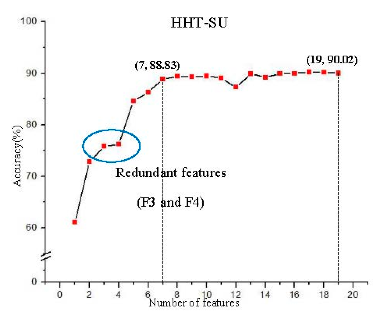
5.4.2. SU Value Screening and Accuracy

Second, this study uses the feature-selection method of SU value to bring in the correlation coefficient for calculation. By obtaining the correlation between features and categories, the features will gradually obtain recognition results from high to low correlation. It is found that when the number of features reaches 7, the accuracy of this method tends to be stable. Moreover, it can be reduced to 19 features (76.25% of the total number of features can be deleted). After all features are identified, the recognition result can be increased from 88.83% to 90.2%, as shown in Figure 13. However, this method is the same as ReliefF, and it also cannot remove redundant features, so there are still a few features with more influence to affect the accuracy of classification.

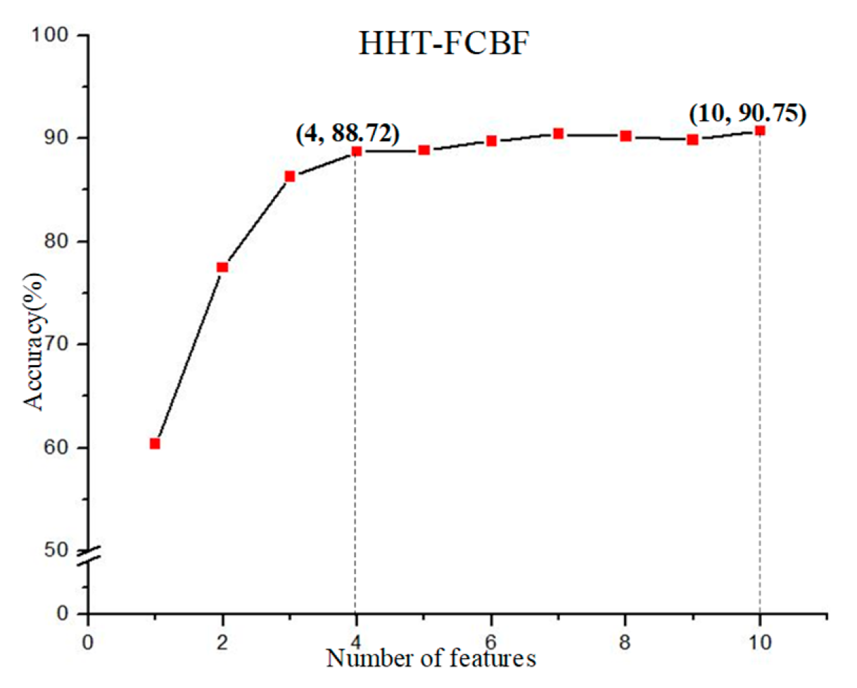
5.4.3. FCBF Screening and Accuracy

Finally, this study uses the feature selection mechanism of FCBF to select the features after analysis. The results indicate that this feature-selection method cannot only effectively delete features with less influence, but also compare features with extremely high correlation. In this way, a two-stage screening process is performed to reduce the number of features. While comparing it can delete redundant features in a short period of time, quickly achieve balance and obtain better recognition results. For the FCBF method, the selected features are gradually identified from important to relatively unimportant features. It was found that the number of features was reduced from 80 features originally analyzed using HHT to 10 features (87.5% of the total number of features was deleted). When using the classifier to calculate its accuracy, when the number of features reaches 4, the accuracy of this method tends to be stable. Moreover, when gradually completed, the accuracy of all features can be effectively increased from 88.72% to 90.75%, as shown in Figure 14. This shows that this screening method can obtain important features compared to the first two and delete unnecessary features that affect the classification to maintain effective identification.

5.4.4. Influence of Various Characteristics on Accuracy

This section mainly discusses the important features by each feature-selection method, which may be different due to the basis of each method screening, so that the number of important features and feature numbers also have different results. Therefore, this study ranks the importance of the features selected by the three different methods. It can be found that the importance and number of features are also not the same due to the different amount of noise, as shown in

Table 9. Importance and quantity of screening features.

Analytical Method	Noise	Methods	Number of Features	Sort by Important Features after Screening (The Redundant Features are Bold)
HHT	$\infty$ dB	ReliefF	22	F5, F45, F3, F1, F42, F2, F4, F16, F44, F43, F41, F61, F30, F6, F15, F33, F29, F77, F65, F26, F66, F55
		SU	19	F41, F43, F44, F42, F45, F5, F1, F2, F4, F31, F49, F11, F3, F38, F67, F56, F48, F30, F15
		FCBF	10	F41, F45, F5, F4, F31, F49, F11, F38, F67, F30
	40 dB	ReliefF	28	F3, F5, F45, F1, F42, F5, F44, F43, F2, F31, F56, F26, F23, F6, F28, F37, F66, F53, F13, F14, F16, F35, F63, F54, F51, F41, F60, F33
		SU	19	F41, F43, F44, F42, F45, F5, F1, F4, F2, F69, F33, F25, F80, F3, F54, F35, F67, F22, F40
		FCBF	11	F41, F45, F5, F4, F2, F69, F33, F25, F80, F67, F22
	30 dB	ReliefF	34	F3, F5, F45, F1, F38, F42, F28, F44, F4, F43, F26, F29, F30, F63, F46, F16, F37, F51, F8, F6, F75, F9, F20, F61, F10, F11, F48, F41, F15, F64, F50, F40, F68, F49
		SU	24	F43, F44, F41, F42, F45, F5, F4, F3, F16, F72, F58, F1, F59, F27, F71, F76, F6, F32, F37, F78, F62, F68, F70, F56
		FCBF	13	F43, F42, F45, F4, F16, F72, F58, F27, F71, F76, F6, F37, F62
	20 dB	ReliefF	49	F3, F45, F5, F11, F42, F44, F6, F43, F15, F55, F67, F19, F18, F21, F60, F51, F8, F40, F56, F1, F4, F70, F37, F10, F23, F26, F72, F62, F9, F66, F16, F61, F2, F25, F22, F24, F30, F20, F54, F53, F39, F48, F50, F29, F36, F73, F69, F46, F76
		SU	29	F43, F44, F45, F42, F41, F4, F74, F10, F76, F65, F11, F9, F3, F78, F8, F73, F22, F80, F63, F29, F64, F72, F5, F79, F46, F19, F30, F14, F69
		FCBF	15	F43, F45, F42, F41, F4, F74, F10, F65, F11, F22, F80, F29, F46, F14, F69

. By comparing the features in Table 9 with Figure 13 and Figure 14, it can be found that the algorithm of SU value have redundant features compared to FCBF. Hence, we marked the redundant features are bold.

The FCBF–PSO method proposed by this research, PSO features weights for the important features after screening. This method retains all FCBF screening features and uses PSO to optimize the weights of the screening features. Compared with the pre-screening, the accuracy is increased by 4.59%, and the total number of features of 87.5% can be deleted. Simulate the many influencing factors of the actual operating environment of the motor, this study also added white noise of 40 dB, 30 dB and 20 dB to the initial measurement signal for research. Experimental results show that the method has obvious feature deletion under 40-dB and 30-dB noise conditions. Eleven and 13 important features can be obtained, respectively, and the accuracy can reach 91.76% and 83.76%. When the noise is 20 dB, the number of features is reduced to 15 after screening, and the recognition result is significantly reduced, but the accuracy of 72.68% can still be maintained. The comparison between the classifier and the number of features shows that the FCBF–PSO method proposed in this study is the best, as shown in

Table 10. Comparison of the number of features and identification results with this research method.

SNR(dB)	Without Feature Selection		Feature-Selection Methods								Compare FCBF–PSO with HHT
			Typical Feature-Selection Methods						New Method
			ReliefF		SU		FCBF		FCBF–PSO
	Number of Features	Acc (%)	Number of Features	Acc (%)	Number of Features	Acc (%)	Number of Features	Acc (%)	Number of Features	Acc (%)	Acc (%)
$\infty$	80	88.26	22	90.05	19	90.02	10	90.75	10	92.85	+4.59
40	80	87.25	28	88.35	19	85.87	11	88.86	11	91.76	+4.51
30	80	80.64	34	82.06	24	81.08	13	81.62	13	83.76	+3.12
20	80	69.66	49	71.42	29	70.35	15	69.84	15	72.68	+3.02

.

6. Conclusions

This study classifies the current signals of normal, bearing damage, broken rotor bar and short circuits in stator windings of AC induction motors. Among them, we used the signal extractor to capture the current signal of the motor and use HHT to extract its maximum, minimum, average, root mean square and standard deviation features. In addition, we propose feature-selection methods for comparison, including ReliefF that gives feature weights, calculation of SU value indicating the degree of feature influence and FCBF to delete redundant features. Finally, we combined the PSO to optimize the weight of important features and tested the system’s noise immunity by adding white noise. We repeated results calculations 200 times to obtain an average accuracy and performed the feature-selection method multiple times. The results showed stable numbers in both features and accuracy. Moreover, using FCBF–PSO to optimize feature weights to identify fault types had better results. The following are the main research results of this study:

• In this study, through the comparison of feature-selection methods, ReliefF, SU value and FCBF were used to improve the invalid or poor features on the classifier. Under normal circumstances, the number of features decreased by 72.5%, 76.25% and 87.5%, respectively. In terms of accuracy of classification, only the SU method values decreased slightly by 1.16%. The other two feature screening methods were optimized. When adding severe noise (SNR = 20 dB), the number of features of the three screening feature methods improved. As far as accuracy was concerned, in addition to the obvious improvement of FCBF, the other two methods still could achieve more than 70% classification ability.
• This study also used a PSO optimization model to optimize the feature weights of the three-phase induction motor signals obtained by the FCBF feature-selection method. This method also preserved all the features of FCBF. Under normal circumstances, its classification accuracy through BPNN could reach 92.85%, which was superior to other feature-selection methods. It also improved the accuracy of 4.59% higher than that of HHT. Then doping it with different noise SNR = 40 dB, SNR = 30 dB and SNR = 20 dB white noise, its accuracy also increased by 4.51%, 3.12% and 3.02%. Therefore, it was shown that this method could obtain a higher classification accuracy.

References

1. Bazurto, A.J.; Quispe, E.C.; Mendoza, R.C. Causes and failures classification of industrial electric motor. In Proceedings of the 2016 IEEE ANDESCON, Arequipa, Peru, 19–21 October 2016; pp. 1–4. [Google Scholar] [CrossRef]
2. Susaki, H. A fast algorithm for high-accuracy frequency measurement: Application to ultrasonic Doppler sonar. IEEE J. Ocean. Eng. 2002, 27, 5–12. [Google Scholar] [CrossRef]
3. Borras, D.; Castilla, M.; Moreno, N.; Montano, J.C. Wavelet and neural structure: A new tool for diagnostic of power system disturbances. IEEE Trans. Ind. Appl. 2001, 37, 184–190. [Google Scholar] [CrossRef]
4. Jin, N.; Liu, D.-R. Wavelet Basis Function Neural Networks for Sequential Learning. IEEE Trans. Neural Netw. 2008, 19, 523–528. [Google Scholar] [CrossRef] [PubMed]
5. Perera, N.; Rajapakse, A.D. Recognition of fault transients using a probabilistic neural-network classifier. IEEE Trans. Power Deliv. 2010, 26, 410–419. [Google Scholar] [CrossRef]
6. Tripathy, M.; Maheshwari, R.; Verma, H. Power Transformer Differential Protection Based On Optimal Probabilistic Neural Network. IEEE Trans. Power Deliv. 2009, 25, 102–112. [Google Scholar] [CrossRef]
7. Ying, S.; Jianguo, Q. A Method of Arc Priority Determination Based on Back-Propagation Neural Network. In Proceedings of the 2017 4th International Conference on Information Science and Control Engineering (ICISCE), Changsha, China, 21–23 July 2017; pp. 38–41. [Google Scholar]
8. Wu, W.; Feng, G.; Li, Z.; Xu, Y. Deterministic Convergence of an Online Gradient Method for BP Neural Networks. IEEE Trans. Neural Netw. 2005, 16, 533–540. [Google Scholar] [CrossRef] [PubMed]
9. Yu, L.; Liu, H. Efficient feature selection via analysis of relevance and redundancy. J. Mach. Learn. Res. 2004, 5, 1205–1224. [Google Scholar]
10. Robnik-Šikonja, M.; Kononenko, I. Theoretical and empirical analysis of ReliefF and RReliefF. Mach. Learn. 2003, 53, 23–69. [Google Scholar] [CrossRef] [Green Version]
11. Senliol, B.; Gulgezen, G.; Yu, L.; Çataltepe, Z. Fast Correlation Based Filter (FCBF) with a different search strategy. In Proceedings of the 2008 23rd International Symposium on Computer and Information Sciences, Istanbul, Turkey, 27–29 October 2008; pp. 1–4. [Google Scholar] [CrossRef]
12. Ishaque, K.; Salam, Z. A Deterministic Particle Swarm Optimization Maximum Power Point Tracker for Photovoltaic System under Partial Shading Condition. IEEE Trans. Ind. Electron. 2012, 60, 3195–3206. [Google Scholar] [CrossRef]
13. Huang, N.E.; Shen, Z.; Long, S.R.; Wu, M.C.; Shih, H.H.; Zheng, Q.; Yen, N.-C.; Tung, C.C.; Liu, H.H. The empirical mode decomposition and the Hilbert spectrum for nonlinear and non-stationary time series analysis. Proc. R. Soc. A Math. Phys. Eng. Sci. 1998, 454, 903–995. [Google Scholar] [CrossRef]
14. Zhang, H.; Wang, F.; Jia, D.; Liu, T.; Zhang, Y. Automatic Interference Term Retrieval from Spectral Domain Low-Coherence Interferometry Using the EEMD-EMD-Based Method. IEEE Photonics-J. 2016, 8, 1–9. [Google Scholar] [CrossRef]
15. Kijewski-Correa, T.; Kareem, A. Efficacy of Hilbert and Wavelet Transforms for Time-Frequency Analysis. J. Eng. Mech. 2006, 132, 1037–1049. [Google Scholar] [CrossRef]
16. Sharma, V.; Rai, S.; Dev, A. A Comprehensive Study of Artificial Neural Networks. Int. J. Adv. Res. Comput. Sci. Softw. Eng. 2012, 2, 278–284. [Google Scholar]
17. Kumar, A.; Tyagi, N. Comparative analysis of backpropagation and RBF neural network on monthly rainfall prediction. In Proceedings of the 2016 International Conference on Inventive Computation Technologies (ICICT), Coimbatore, India, 26–27 August 2016; Volume 1, pp. 1–6. [Google Scholar]
18. Upadhyay, P.K.; Pandita, A.; Joshi, N. Scaled Conjugate Gradient Backpropagation based SLA Violation Prediction in Cloud Computing. In Proceedings of the 2019 International Conference on Computational Intelligence and Knowledge Economy (ICCIKE), Dubai, UAE, 11–12 December 2019; pp. 203–208. [Google Scholar]
19. Xue, B.; Zhang, M.; Browne, W.N.; Yao, X. A Survey on Evolutionary Computation Approaches to Feature Selection. IEEE Trans. Evol. Comput. 2015, 20, 606–626. [Google Scholar] [CrossRef] [Green Version]
20. Ang, J.C.; Mirzal, A.; Haron, H.; Hamed, H.N.A. Supervised, Unsupervised, and Semi-Supervised Feature Selection: A Review on Gene Selection. IEEE/ACM Trans. Comput. Biol. Bioinform. 2015, 13, 971–989. [Google Scholar] [CrossRef] [PubMed]
21. Gopika, N.; Kowshalaya, A.M.M.E. Correlation Based Feature Selection Algorithm for Machine Learning. In Proceedings of the 2018 3rd International Conference on Communication and Electronics Systems (ICCES), Coimbatore, India, 15–16 October 2018; pp. 692–695. [Google Scholar]
22. Sawhney, H.; Jeyasurya, B. A feed-forward artificial neural network with enhanced feature selection for power system transient stability assessment. Electr. Power Syst. Res. 2006, 76, 1047–1054. [Google Scholar] [CrossRef]
23. Song, Q.; Ni, J.; Wang, G. A Fast Clustering-Based Feature Subset Selection Algorithm for High-Dimensional Data. IEEE Trans. Knowl. Data Eng. 2011, 25, 1–14. [Google Scholar] [CrossRef]
24. Yu, L.; Liu, H. Feature Selection for High-Dimensional Data: A Fast Correlation-Based Filter Solution. In Proceedings of the Twentieth International Conference on Machine Learning, Washington, DC, USA, 21–24 August 2003; pp. 856–863. [Google Scholar]
25. Kononenko, I.; Šimec, E.; Robnik-Šikonja, M. Overcoming the Myopia of Inductive Learning Algorithms with RELIEFF. Appl. Intell. 1997, 7, 39–55. [Google Scholar] [CrossRef]
26. Armay, E.F.; Wahid, I. Entropy simulation of digital information sources and the effect on information source rates. In Proceedings of the 2011 2nd International Conference on Instrumentation, Communications, Information Technology, and Biomedical Engineering, Bandung, Indonesia, 8–9 November 2011; pp. 74–78. [Google Scholar]
27. Hall, M.A. Correlation Based Feature Selection for Machine Learning. Ph.D. Thesis, University of Waikato, Hamilton, NewZealand, 1999. [Google Scholar]
28. Djellali, H.; Guessoum, S.; Ghoualmi-Zine, N.; Layachi, S. Fast correlation based filter combined with genetic algorithm and particle swarm on feature selection. In Proceedings of the 2017 5th International Conference on Electrical Engineering-Boumerdes (ICEE-B), Boumerdes, Algeria, 29–31 October 2017; pp. 1–6. [Google Scholar]
29. Lee, C.-Y.; Tuegeh, M. Optimal optimisation-based microgrid scheduling considering impacts of unexpected forecast errors due to the uncertainty of renewable generation and loads fluctuation. IET Renew. Power Gener. 2020, 14, 321–331. [Google Scholar] [CrossRef]
Figure 1. Flowchart of EMD.
Applsci 10 05383 g001
Figure 2. Feature selection method and application.
Applsci 10 05383 g002
Figure 3. Classifications based on relevancy and redundancy.
Applsci 10 05383 g003
Figure 4. Method of fast correlation-based filter (FCBF) delete redundant feature.
Applsci 10 05383 g004
Figure 5. Flowchart of FCBF feature selection.
Applsci 10 05383 g005
Figure 6. Flowchart of FCBF–PSO method.
Applsci 10 05383 g006
Figure 7. (a) Bearing damage motor (aperture: 1.96 mm × 0.53 mm) (b) schematic diagram of bearing damage (c) broken rotor bar motor (2 holes ~8 mm deep: 10 mm) (d) schematic diagram of broken rotor bar (e) short circuit in stator windings motor (2 coil short circuit) (f) short circuit model in stator (g) power test platform.
Applsci 10 05383 g007
Figure 8. (a) Setup of actual measurement (b) flowchart of experimental architecture.
Applsci 10 05383 g008
Figure 9. (a) Original signal from healthy motor and (b) component after using empirical mode decomposition (EMD).
Applsci 10 05383 g009
Figure 10. Architecture diagram of Hilbert–Huang transform (HHT) extraction features.
Applsci 10 05383 g010
Figure 11. (a) Feature distribution of motor failure ( dB); (b) feature distribution of motor failure (20 dB).
Applsci 10 05383 g011
Figure 12. ReliefF method and accuracy.
Applsci 10 05383 g012
Figure 13. Symmetrical uncertainty (SU) value method and accuracy.
Applsci 10 05383 g013
Figure 14. FCBF method and accuracy.
Applsci 10 05383 g014