Figure 1.
Rotating and outer domain: (a) rotation domain for wind turbine simulation; (b) entire computational domain for numerical simulation.
Figure 1.
Rotating and outer domain: (a) rotation domain for wind turbine simulation; (b) entire computational domain for numerical simulation.
Figure 2.
The computational mesh domain for the wind turbine: (a) full grid domain, (b) sliding mesh regions, (c) close-up view of the blade surface, (d) close-up view of the hub surface mesh and (e) close-up view of nacelle and tower.
Figure 2.
The computational mesh domain for the wind turbine: (a) full grid domain, (b) sliding mesh regions, (c) close-up view of the blade surface, (d) close-up view of the hub surface mesh and (e) close-up view of nacelle and tower.
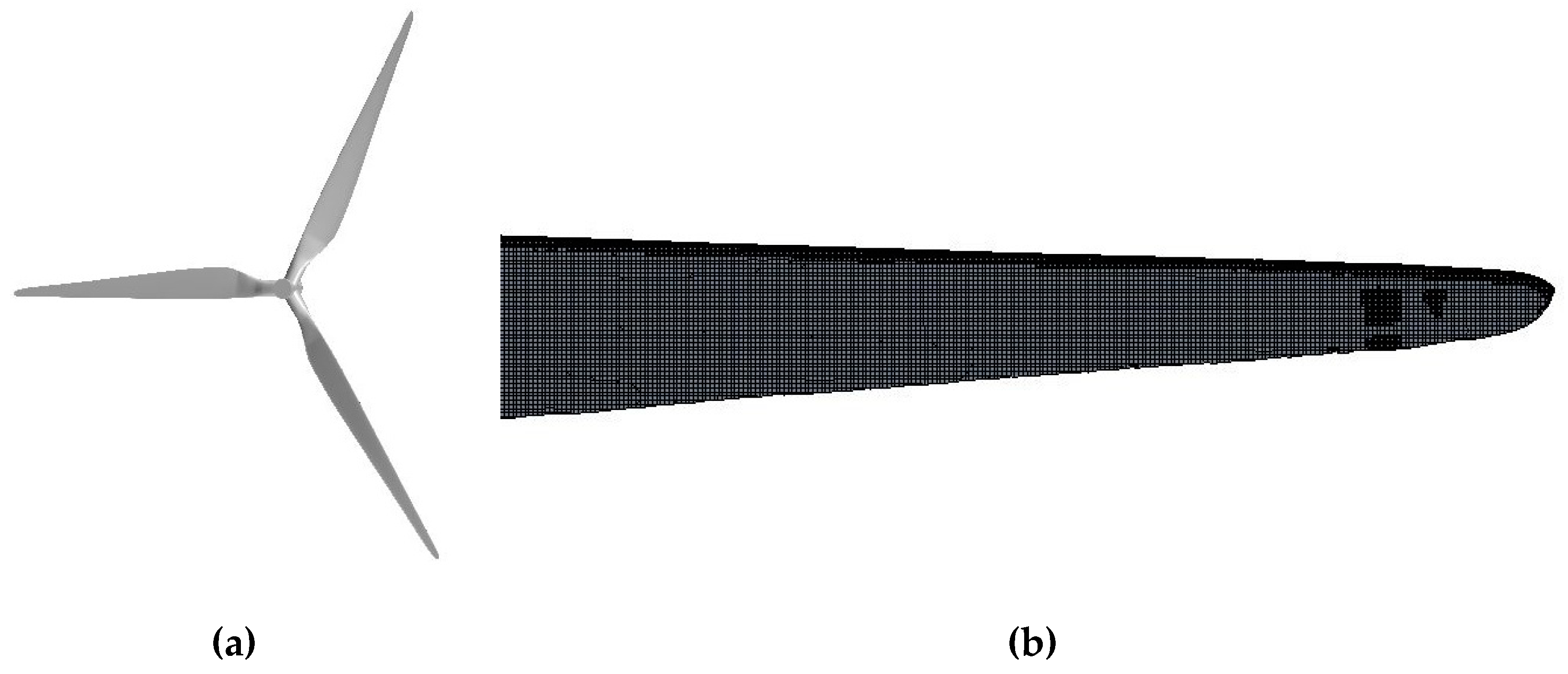
Figure 3.
Geometric model and surface grid: (a) the rotor geometric model; (b) the blade surface grid.
Figure 3.
Geometric model and surface grid: (a) the rotor geometric model; (b) the blade surface grid.
Figure 4.
Comparison of thrust and torque between wind tunnel experiment and CFD simulation at different wind speeds (Case 3).
Figure 4.
Comparison of thrust and torque between wind tunnel experiment and CFD simulation at different wind speeds (Case 3).
Figure 5.
Geometric model of a 5 MW reference wind turbine: (a) the rotor geometric model; (b) the full configuration model.
Figure 5.
Geometric model of a 5 MW reference wind turbine: (a) the rotor geometric model; (b) the full configuration model.
Figure 6.
Comparisons of thrust and power.
Figure 6.
Comparisons of thrust and power.
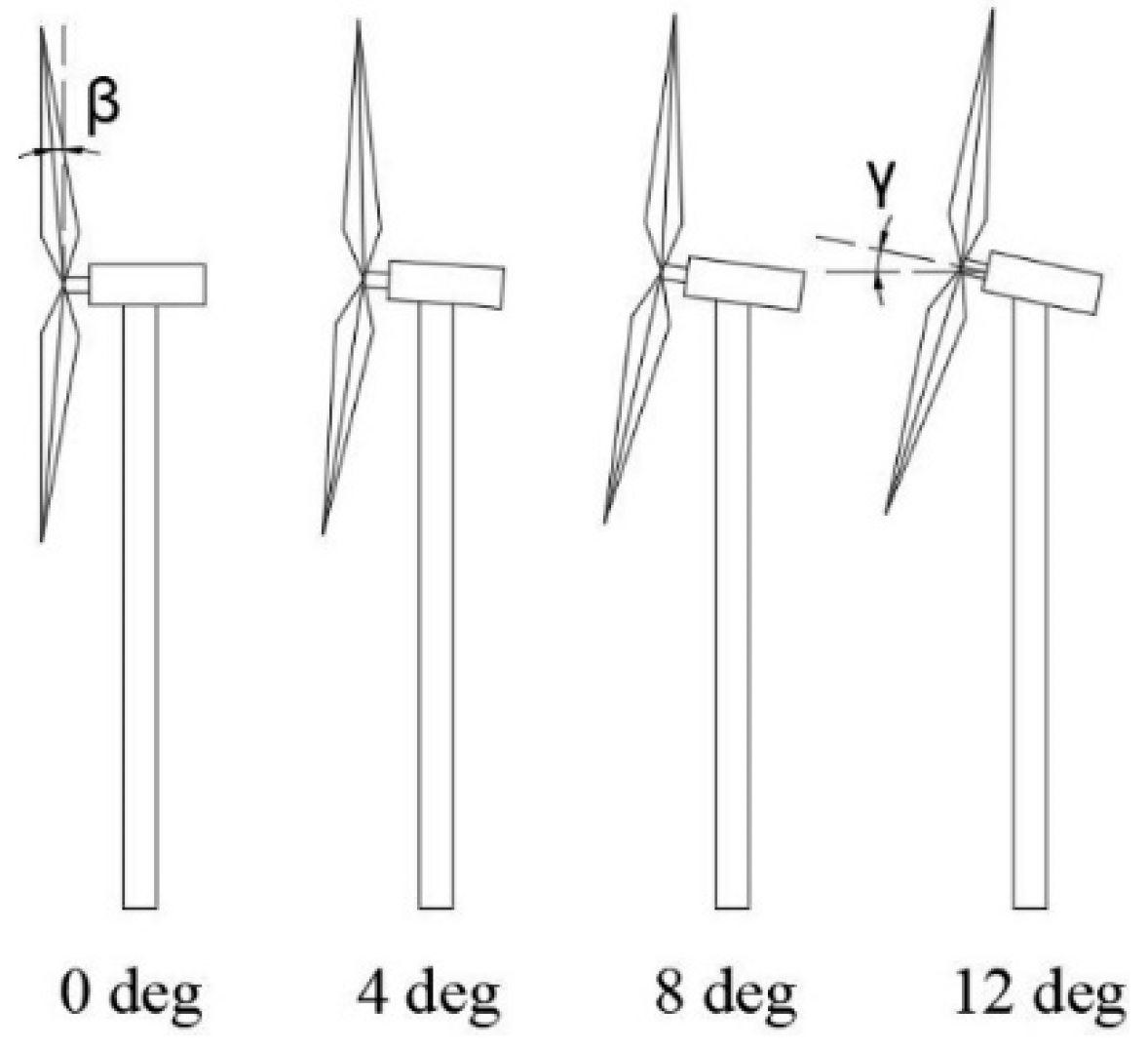
Figure 7.
Structure of the wind turbine at different tilt angles.
Figure 7.
Structure of the wind turbine at different tilt angles.
Figure 8.
Definition of the azimuth.
Figure 8.
Definition of the azimuth.
Figure 9.
Comparison of thrust and power at different nacelle tilt angles.
Figure 9.
Comparison of thrust and power at different nacelle tilt angles.
Figure 10.
Comparison of thrust and power at different nacelle tilt angles (partial enlargement).
Figure 10.
Comparison of thrust and power at different nacelle tilt angles (partial enlargement).
Figure 11.
Blade position (ψ = 60°).
Figure 11.
Blade position (ψ = 60°).
Figure 12.
Instantaneous pressure magnitude and streamlines diagram (r/R = 0.5).
Figure 12.
Instantaneous pressure magnitude and streamlines diagram (r/R = 0.5).
Figure 13.
Instantaneous pressure magnitude and streamlines diagram (r/R = 0.7).
Figure 13.
Instantaneous pressure magnitude and streamlines diagram (r/R = 0.7).
Figure 14.
Instantaneous pressure magnitude and streamlines diagram (r/R = 0.9).
Figure 14.
Instantaneous pressure magnitude and streamlines diagram (r/R = 0.9).
Figure 15.
The average thrust and average tangential force per unit of span along the blade span for Blade 1.
Figure 15.
The average thrust and average tangential force per unit of span along the blade span for Blade 1.
Figure 16.
Thrust and tangential force per unit of span along the blade span for Blade 1.
Figure 16.
Thrust and tangential force per unit of span along the blade span for Blade 1.
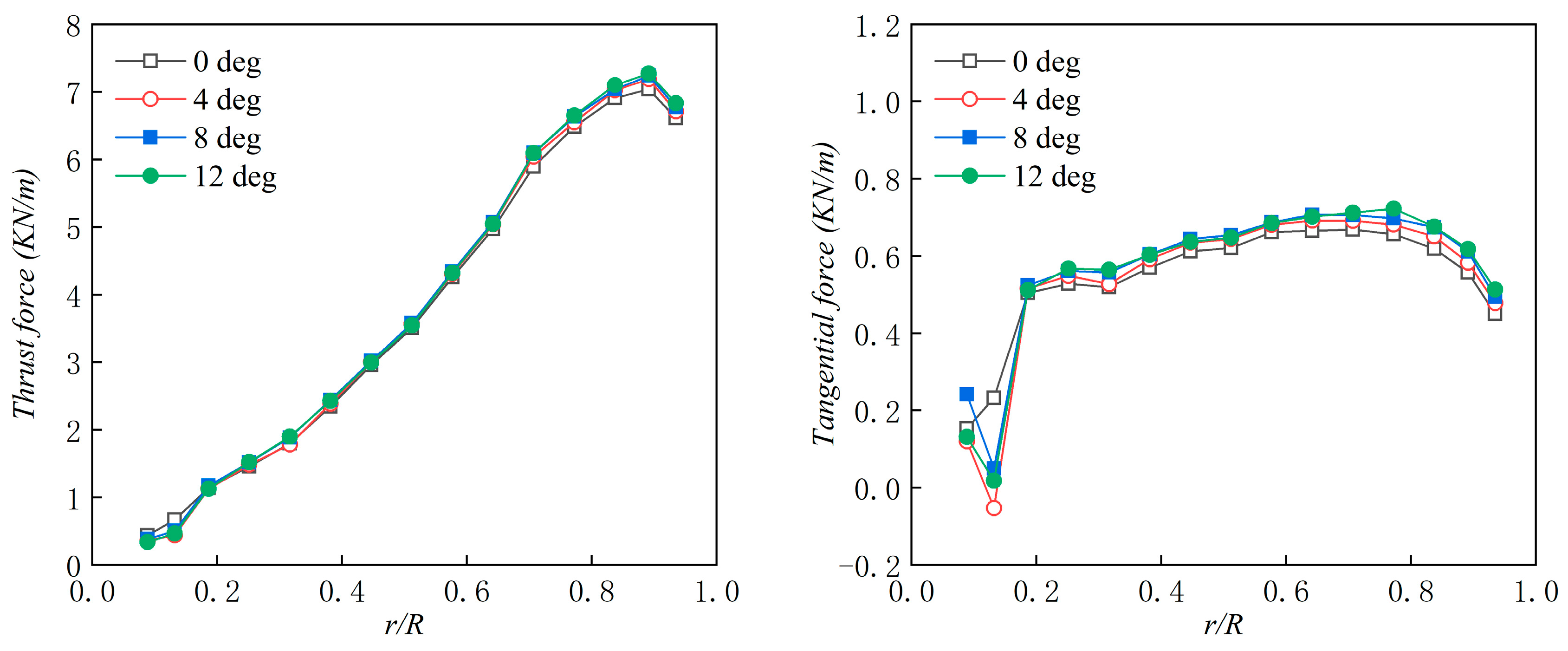
Figure 17.
Thrust force per unit of span along the rotor span for Blade 1.
Figure 17.
Thrust force per unit of span along the rotor span for Blade 1.
Figure 18.
Tangential force per unit of span along the rotor span for Blade 1.
Figure 18.
Tangential force per unit of span along the rotor span for Blade 1.
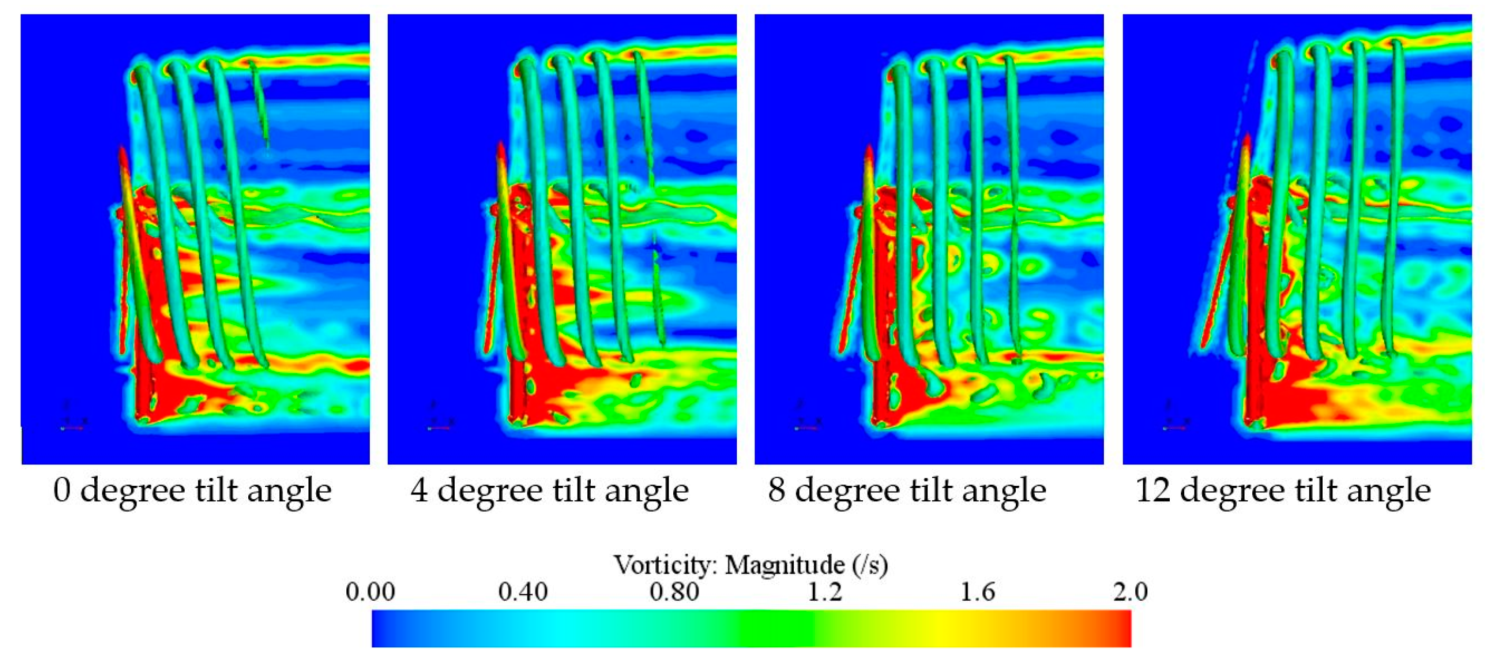
Figure 19.
Side-view of instantaneous isovorticity contours for different nacelle tilt angles.
Figure 19.
Side-view of instantaneous isovorticity contours for different nacelle tilt angles.
Figure 20.
Instantaneous x-vorticities at different sections for four tilt angles.
Figure 20.
Instantaneous x-vorticities at different sections for four tilt angles.
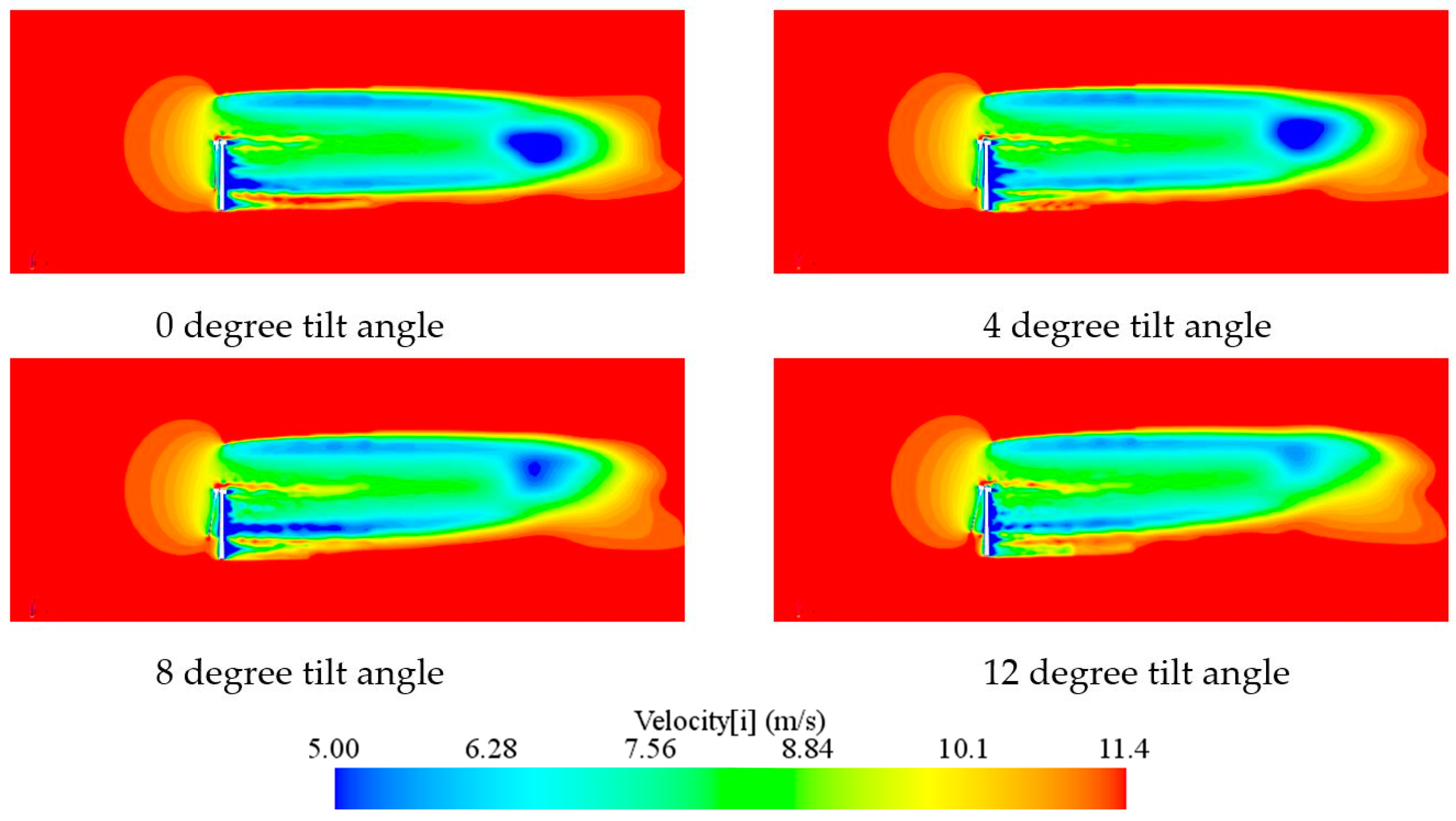
Figure 21.
Vertical section x-velocity profiles at y = 0 m.
Figure 21.
Vertical section x-velocity profiles at y = 0 m.
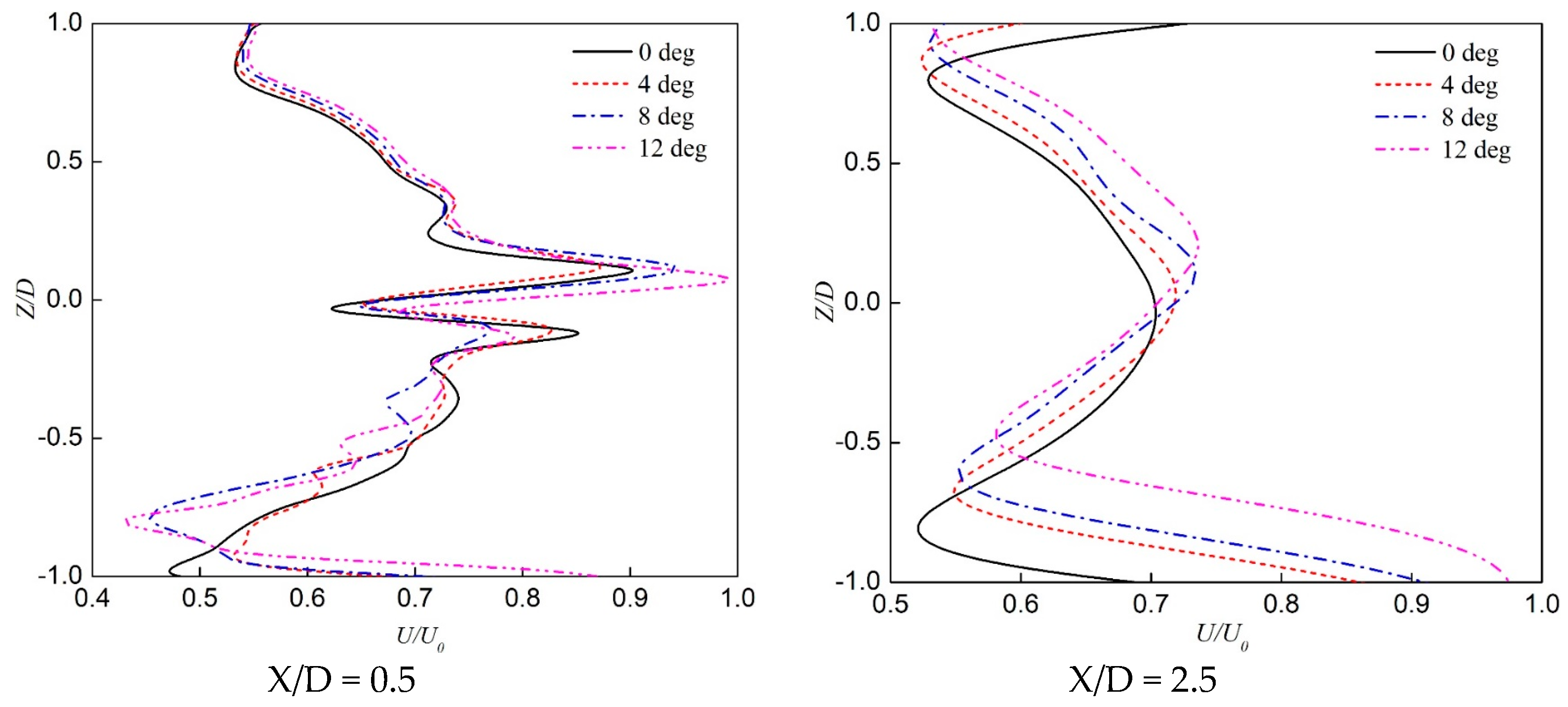
Figure 22.
The distribution of instantaneous axial velocity along blade span at the wind turbine downstream positions of 0.5D, 2.5D, 3.5D and 4.5D.
Figure 22.
The distribution of instantaneous axial velocity along blade span at the wind turbine downstream positions of 0.5D, 2.5D, 3.5D and 4.5D.
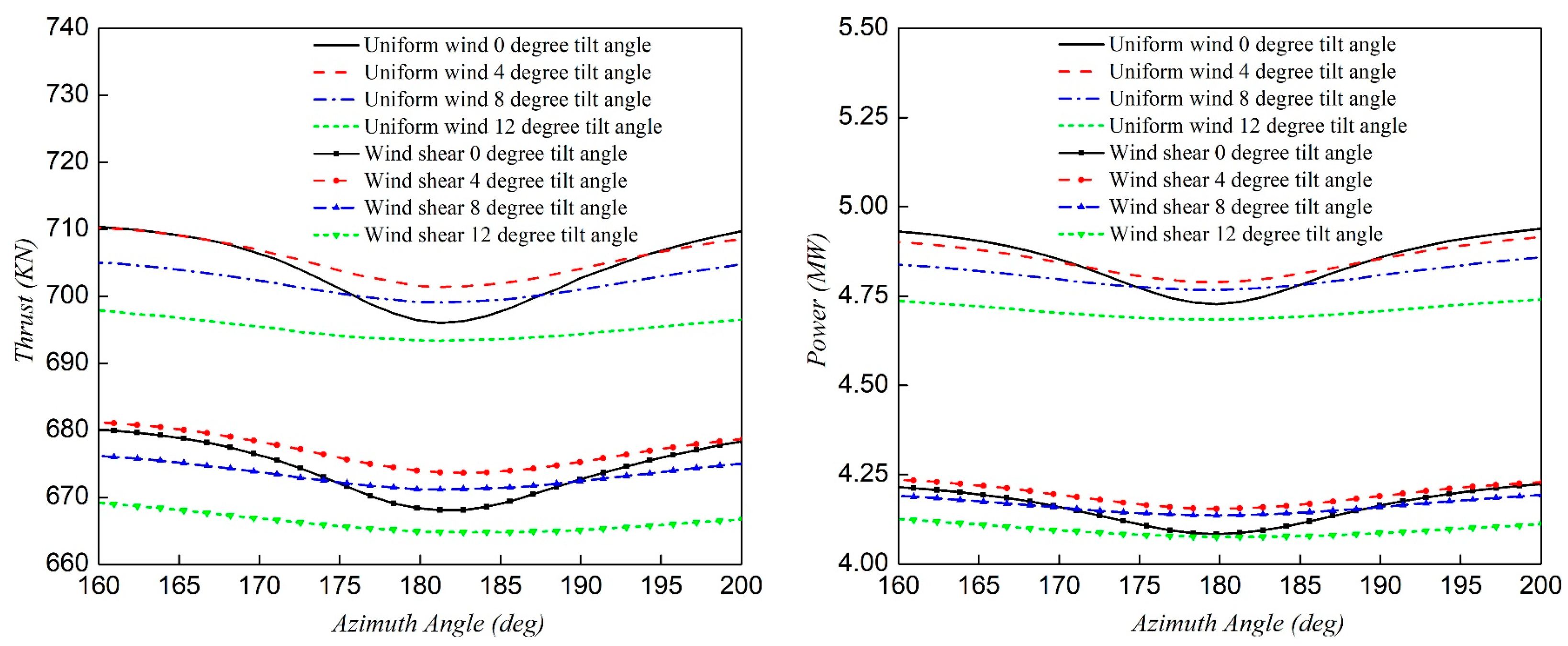
Figure 23.
Thrust and power versus azimuth angle for various tilt angles at = 11.4 m/s (γ = 0.2, = 0.14).
Figure 23.
Thrust and power versus azimuth angle for various tilt angles at = 11.4 m/s (γ = 0.2, = 0.14).
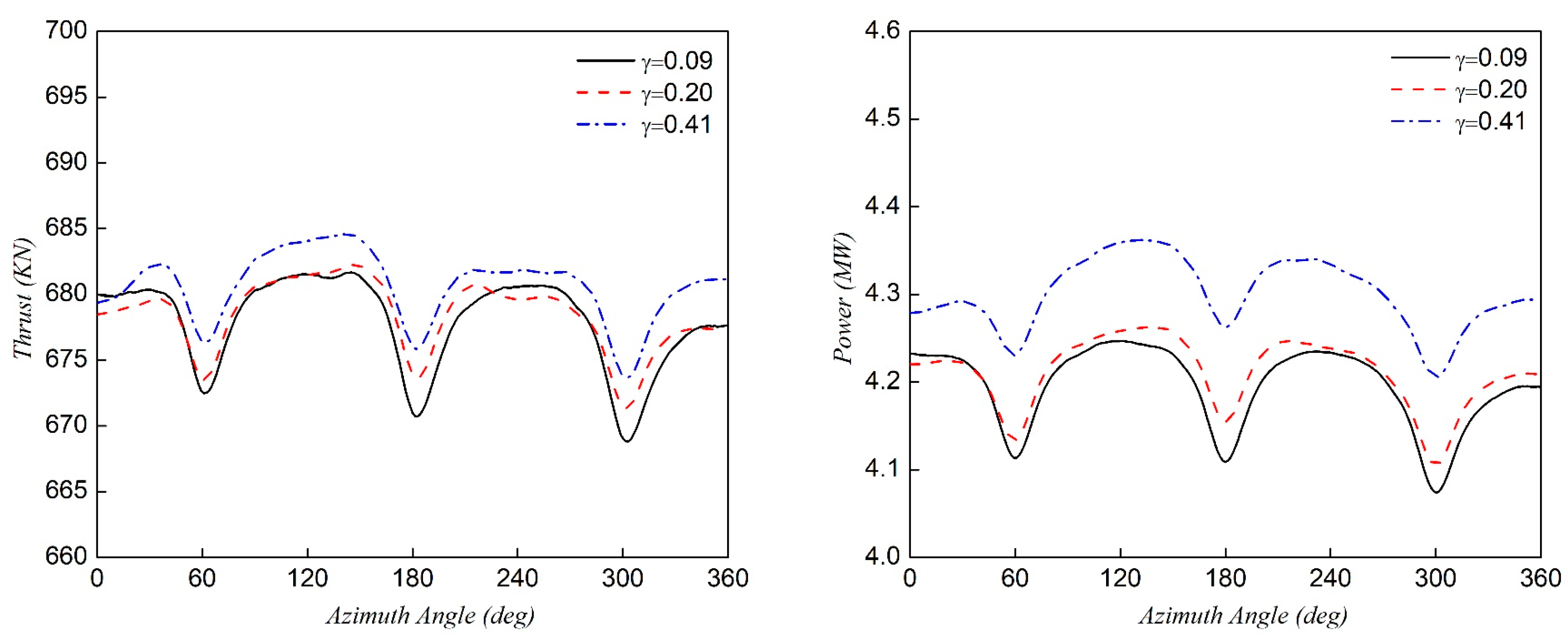
Figure 24.
Thrust and power versus azimuth angle for various wind shear exponents (γ) at = 11.4 m/s ( = 0.14, tilt angle = 4°).
Figure 24.
Thrust and power versus azimuth angle for various wind shear exponents (γ) at = 11.4 m/s ( = 0.14, tilt angle = 4°).
Figure 25.
Thrust and power versus azimuth angle for various expected values of the turbulence intensity () at = 11.4 m/s (γ = 0.2, tilt angle = 4°).
Figure 25.
Thrust and power versus azimuth angle for various expected values of the turbulence intensity () at = 11.4 m/s (γ = 0.2, tilt angle = 4°).
Table 1.
Principal dimensions of the scale model.
Table 1.
Principal dimensions of the scale model.
| Specifications | DTU Down-Scaled |
|---|
| Number of Blades | 3 |
| Rotor Diameter (m) | 2.37 |
| Hub Diameter (m) | 0.178 |
| Rated Wind Speed (m/s) | 5.53 |
| Rated Rotor Speed (rpm) | 330 |
Table 2.
Mesh size of blade surface.
Table 2.
Mesh size of blade surface.
| CFD Mesh Type | Case 1 | Case 2 | Case 3 | Case 4 |
|---|
| Maximum Size (mm) | 3.000 | 2.000 | 1.500 | 1.100 |
| Minimum Size (mm) | 0.500 | 0.350 | 0.250 | 0.180 |
| Total Mesh Number (million) | 1.850 | 3.240 | 4.630 | 9.400 |
Table 3.
Comparison of thrust between experiment and CFD simulation at different grid densities.
Table 3.
Comparison of thrust between experiment and CFD simulation at different grid densities.
| CFD Mesh Type | LIFES50+ Wind Tunnel Data (N), [14] | Present Study (N) | Error (%) |
|---|
| Case 1 | 68.631 | 70.010 | 2.000 |
| Case 2 | 69.660 | 1.500 |
| Case 3 | 69.520 | 1.300 |
| Case 4 | 69.500 | 1.300 |
Table 4.
Comparison of torque between experiment and CFD simulation at different grid densities.
Table 4.
Comparison of torque between experiment and CFD simulation at different grid densities.
| CFD Mesh Type | , [14]
| | Error (%) |
|---|
| Case 1 | 6.232 | 5.690 | 8.700 |
| Case 2 | 5.850 | 6.100 |
| Case 3 | 5.900 | 5.300 |
| Case 4 | 5.920 | 5.000 |
Table 5.
Principal dimensions of the NREL 5 MW reference wind turbine.
Table 5.
Principal dimensions of the NREL 5 MW reference wind turbine.
| Specifications | |
|---|
| Rated Power (MW) | 5 |
| Rotor Orientation, Configuration | Upwind, 3 blades |
| Rated Wind Speed (m/s) | 11.4 |
| Rated Rotor Speed (rpm) | 12.1 |
| Rotor Diameter (m) | 126 |
| Hub Diameter (m) | 3 |
| Hub Height (m) | 90 |
| Tower Base Diameter (m) | 6 |
| Tower Top Diameter (m) | 3.87 |
| Pre-cone (°) | 2.5 |
Table 6.
Mesh size of blade surface.
Table 6.
Mesh size of blade surface.
| CFD Mesh Type | Case 1 | Case 2 | Case 3 |
|---|
| Maximum Size (m) | 0.20 | 0.10 | 0.05 |
| Minimum Size (m) | 0.04 | 0.02 | 0.01 |
| Total Mesh Number (Million) | 1.52 | 4.80 | 9.53 |
Table 7.
Comparison of power between NREL data and CFD simulation at different grid densities.
Table 7.
Comparison of power between NREL data and CFD simulation at different grid densities.
| CFD Mesh Type | NREL Data (MW), [16] | Present Study (N) | Error (%) |
|---|
| Case 1 | 5.000 | 4.767 | 4.700 |
| Case 2 | 4.981 | 0.380 |
| Case 3 | 5.020 | 0.400 |
Table 8.
Power for uniform wind and wind shear flow conditions at = 11.4 m/s (γ = 0.2, = 0.14).
Table 8.
Power for uniform wind and wind shear flow conditions at = 11.4 m/s (γ = 0.2, = 0.14).
| Tilt Angle (°) | Average Power Pa (MW) | Power Pm at 180° Azimuth Angle (MW) | |
|---|
| Uniform Wind | Wind Shear | Error (%) | Uniform Wind | Wind Shear | Error (%) | Uniform Wind | Wind Shear |
|---|
| 0 | 4.92 | 4.20 | 14.63 | 4.73 | 4.08 | 13.74 | 0.19 | 0.12 |
| 4 | 4.91 | 4.21 | 14.26 | 4.79 | 4.15 | 13.36 | 0.12 | 0.06 |
| 8 | 4.85 | 4.18 | 13.81 | 4.78 | 4.14 | 13.39 | 0.07 | 0.04 |
| 12 | 4.75 | 4.12 | 13.26 | 4.68 | 4.08 | 12.82 | 0.07 | 0.04 |
Table 9.
The power for various wind shear exponents (γ) at = 11.4 m/s ( = 0.14, tilt angle = 4°).
Table 9.
The power for various wind shear exponents (γ) at = 11.4 m/s ( = 0.14, tilt angle = 4°).
| Wind Shear Exponents | Average Power Pa (MW) | Average Thrust Ta (KN) |
|---|
| Power | Relatively Uniform Wind Error (%) | Thrust | Relatively Uniform Wind Error (%) |
|---|
| 0.00 | 4.91 | 0.00 | 709.16 | 0.00 |
| 0.09 | 4.19 | 14.66 | 677.89 | 4.41 |
| 0.20 | 4.21 | 14.26 | 678.38 | 4.34 |
| 0.41 | 4.30 | 12.42 | 680.64 | 4.02 |


