Analyzing Six Indices for Online Short-Term Voltage Stability Monitoring in Power Systems

Abstract

In recent years, the importance of online monitoring short-term voltage stability has been considerably increased. Unstable cases due to response of fast dynamic loads such as induction motors to the serious disturbances can be avoided by online monitoring of voltage transients and activating fast and appropriate controls to encounter deep and prolonged voltage drop. In this paper, a set of indices based on the phasor measurement unit (PMU) measurements are introduced and compared for short-term voltage stability. To increase efficiency of the indices, a special algorithm for each index is proposed by using the investigation of the results of applying them to six disturbances’ scenarios simulated on the IEEE 39 bus system. The disturbance scenarios are representative of different cases of stable, unstable, and deep and prolonged voltage drop associated with short-term voltage transients. The performance of these indices are studied in terms of the time and accuracy required for determining the short-term voltage stability/instability cases. It is shown that the proposed method has better performance in comparison with other techniques that can be applied to power systems in reality.

1. Introduction

In recent years, due to the ever-increasing electrical demand and the limitations associated with financial resources, power systems are usually operated near their transmission capability limits [1]. Therefore, new real-time monitoring and control techniques are necessary to guarantee secure operation of modern power systems. One of the main stability issues in modern power system is the voltage stability that needs to be monitored for keeping the system operation in safe mode. Based on time frame of appearance instability, voltage stability problem can be classified into long-term and short-term voltage stability studies [2]. Due to increase of amounts of dynamic loads, especially induction motors, which led to increasing the reactive power demand under reduced-voltage conditions, power systems have become more vulnerable to short-term voltage stability (SVS) problems. Therefore, the monitoring of short-term voltage stability (SVS) has become necessary to be taken into consideration especially for modern power systems and future smart grids [3,4,5].

Short-term voltage instability should be identified to prevent significant voltage drop which might lead to damage of equipment and disruption of power balance and finally might cause a system’s collapse. In [6], an SVS analysis from the perspective of active and reactive power balancing has been proposed.

In the last few decades, model-based methods have been utilized for analyzing short-term voltage stability, in which these methods have focused on the dynamic modeling and aggregation of fast acting load components like induction motor loads [7]. However, model-based methods for SVS monitoring have some difficulties in modeling dynamic loads and setting load parameters. It has been clearly demonstrated that the application of model-based methods in reality might encounter infeasibility due to reasons such as the wide diversity of the used components of the system loads and their different characteristics, and the unavailability of the required load information of all areas in the control center in real-time [4,8]. Therefore, the effectiveness of model-based methods is limited in real-time applications.

With the introduction of a phasor measurement unit (PMU) that acquires time-synchronized measurements at a much higher sampling rate rather than conventional measurement devices, wide-area measurement systems (WAMS) have been widely deployed in reality. Due to deployment of WAMS, the real-time voltage and current phasors become available in control centers which helps in improving the online monitoring and control of modern power systems [9,10]. Therefore, data-based or model-free methods can be adopted and developed for online stability monitoring in modern and future power systems. In data-based methods, PMUs data are used to calculate indices for voltage instability detection. In [11,12], long term voltage stability indicators based on PMU data have been proposed for stability monitoring and can identify critical loads in a system. Recently, Lyapunov exponents (LE) have been extensively used in literature for short-term voltage instability prediction.

In [7], a data-driven method based on the voltage magnitude measured by PMUs has been explained for LE calculation. In [13], the authors have discussed the influence of oscillations and improper parameter settings in instability detection with LE; they proposed an improved phase rectification (PR)-based SVS monitoring method which removes that weakness using modal analysis. In [14], the authors have introduced a framework which uses the PMUs data for calculating LEs. They significantly improved their framework performance under noisy measurements by averaging the latest data packages received in the control center.

Some voltage indices have been suggested in literature and used for dynamic VAR planning based on describing the integration of voltage deviation or the voltage violation time span. These indices have been used for quantifying the short-term voltage stability and the related risk level to optimal placement of dynamic VAR support against short-term voltage instability [15,16,17,18]. In [19], a practical SVS index based on voltage curves has been developed which gives continuous assessment results on the SVS and can be used in the optimization of the offline preventive control for improving the SVS of power systems.

Nowadays, power system operators around the world recommend suggesting new voltage stability indices that can help with improving the overall stability and security in modern power systems. In [15], two voltage severity indices based on NERC/WECC N-1 contingency criteria have been developed. These severity indices utilize PMU data and have been adopted for optimal placement of VAR support in modern power systems. Authors in [17,18] have defined and used a transient voltage severity index to quantify the transient voltage performance of the system buses following the clearance of disturbances. In [16], the stability prediction has been done using the definition of lower and upper reference boundaries for voltage trajectory and calculation trajectory violation integral. In [12], voltage stability index (VSRI) has been used to assess voltage stability. However, the suggested instruction for VSRI needs time intervals of more than 10 seconds so is not suitable for SVS monitoring. It is clear that the aforementioned voltage stability indices suggested in literature are not suitable for short-term voltage stability monitoring due to technical issues limiting their feasibility. Therefore, a research gap in the field of defining suitable short-term voltage stability indices exists that needs to be fulfilled by either applying suitable modifications to the existing long-term voltage stability indices or by suggesting new indices. The main aim of this research is to solve the above-mentioned research gap by modifying the existing indices and by proposing a novel practical index suitable for SVS monitoring.

This paper proposes a novel index for monitoring short-term voltage stability in modern power systems. Likewise, the paper reviews the existing short-term voltage stability indices and compares them with each-other and with the proposed novel index for determining the most suitable and feasible index for implementation in reality. The main aim of this work is to gather and provide appropriate voltage indices which are used in literature for different applications (other than SVS applications) and then to investigate their ability in SVS monitoring and assessment. The paper focuses on the simply computed SVS indices that can be adopted in reality and to avoid any complexities and unpractical techniques. In addition, with applying appropriate modifications and changes, six simple computing voltage indices for SVS monitoring using online measurement PMU data are introduced. Most of these indices are used in literature for reactive power planning and one of them is used as a long-term voltage index, but they have never been introduced for SVS monitoring and assessment. By applying these indices for six scenarios related to SVS phenomena that are obtained from simulations on a 39-bus test system, simple instructions are developed for using these indices as proper indices for SVS monitoring. To compare the reliability and speed of proposed indices, a suitable database is generated by simulations, and indices’ abilities in short-term voltage instability detection are obtained and compared with each other. Results show that proposed SVS indices have good performance in SVS monitoring and assessment. The main contributions of this paper are:

• The proposal of novel data-based short-term voltage stability method for modern power systems.
• The ability assessment of reactive power stability compensation and long-term stability indices for SVS monitoring in modern power systems.
• Modifying traditional voltage stability indices to be able for assessing SVS in smart grids.
• Evaluating six different indices for SVS in the power system and selecting the most appropriate one.

The organization of the paper is as follows. The SVS indices are reviewed and their mathematical formulas are presented in Section 2. In Section 3, first, six suitable scenarios are defined and obtained using simulations; then, SVS indices are applied for scenarios to extract their corresponding instructions for SVS monitoring. For assessing SVS indices with their instructions, a database is generated and these indices’ errors in SVS monitoring are obtained and compared in Section 4. Finally in Section 5, conclusions are presented.

2. Mathematical Preliminaries: SVS Indices

As aforementioned, this paper aims to investigate short-term voltage stability monitoring techniques and to propose a new SVS technique using data based methods. It has been focused on the simply computed SVS indices which have acceptable reliability and speed from the short-term instability detection viewpoint. In this section, Lyapunov exponents as an important SVS index are studied first; Then, five other voltage indices are introduced and are then modified for power system SVS monitoring by adopting proper changes.

2.1. Lyapunov Exponents

One of the introduced indices for SVS monitoring is a Lyapunov exponent, which is adapted from ergodic theory of dynamic systems. LEs in nonlinear systems can be considered as eigenvalues in linear systems. The purpose of using LEs in the SVS monitoring is voltage stability/instability prediction by investigation of converging/diverging voltage trajectories. If maximum LEs of the system are positive/negative, it implies convergence/divergence of nearby system trajectories [7].

The following algorithm is used for calculating system LE using measurement data from PMU.

• Consider $V_t=[v_1\left(t\right),v_2\left(t\right),\cdots ,v_n\left(t\right)]$ as voltage time series vector measured by PMU or obtained from simulations, at n buses of system in times $t=0,\Delta t,2\Delta t,\cdots ,M\Delta t$. $\Delta t$ is the sampling period of PMU measurement.
• Choose N initial value of the time series that are satisfied in the following relation:

  $${\epsilon }_1<∥V_{m\Delta t}-V_{(m-1)\Delta t}∥<{\epsilon }_2\begin{array}{c},m=1,2,\cdots ,N\end{array}$$

  (1)

  ${\epsilon }_1,{\epsilon }_2$ are two small fixed numbers and $0<{\epsilon }_1<{\epsilon }_2$.
• For $k=1,2,\cdots ,M$ the maximum Lyapunov exponent at time $k\Delta t$ is defined as follows:

  $$\begin{array}{c}\mathsf{\Lambda }(k\Delta t)=\frac{1}{Nk\Delta t}\times {\displaystyle \sum _{m=1}^N}log\frac{\Vert V(k+m)\Delta t-V(k+m-1)\Delta t\Vert }{\Vert V\left(m\right)\Delta t-V(m-1)\Delta t\Vert }\hfill \\ k>N\hfill \end{array}$$

  (2)

In Equation (2), by taking N initial condition from measurement data and studying its evolution over time, the system’s LE would be calculated. LE in time t is calculated by normalizing distance between N initial conditions at time t to this distance at time zero and averaged over the number of initial conditions. With n PMU in the system that measures n buses voltage and by taking measured quantities after fault clearing time, there are n voltage time series. In [7], it has been proven that system LE is more than maximum individual buses LE. Therefore, it is sufficient to use system LE for instability detection.

For the purpose of online implementation, the Lyapunov exponent needs to be computed over a finite time window [7]. The appropriate size of this window will be crucial for reliable, accurate, and timely stability monitoring depending on considered stability study. In particular, a smaller size window will lead to inaccurate stability prediction, while a larger size window will lead to accurate, but untimely prediction. There exists an optimal window that provides reliable and timely stability predictions. The optimal window depends on fault and system characteristics [7]. Thus, the basic LE algorithm can be improved to avoid oscillation issues by selecting the optimal or suitable parameters and computation window through systematic or empirical methods such as those have been in [13,20]. For example, the LE is estimated by a recursive least squares based method in [13,20], and two critical parameters, the computation window and the LE estimation initial time step, are carefully chosen or, in [13,20], a phase rectification method has been proposed to eliminate the negative influence of oscillation of LE. These methods improve the LE performance in the cost of increasing method complexity and serving a considerable time for setting parameters for a specific system and a specific stability study.

2.2. Contingency Severity Indices (CSI)

According to NERC/WECC Planing Standards, voltage dip should not exceed 25% at load buses and 30% at other buses; in addition, it should not be more than 20% during 20 cycles or more in $N-1$ contingencies [21]. Based on this criteria, two severity indices are used in [15]. The first of them is $S{I}_v$ that is used to quantify voltage limit violation and calculated for each bus at time t as follows:

If $D=\left\{v\left(t\right)|t\in [t_{cl},t_f]\right\}$ ($t_{cl}$ is fault clearing time, and $t_f$ is the time that is considered for short-time voltage stability study) and if there is a $v_{dev}$ in D that is satisfied in relation (3):

$$|v_0-v\left(t\right)|\le |v_0-v_{dev}|\begin{array}{cc}& \forall v\left(t\right)\in D\end{array}$$

(3)

${SI}_v\left(t_f\right)$ for load buses is:

$$S{I}_v\left(t_f\right)=\left\{\begin{array}{c}\begin{array}{c}\left|v_0-v_{dev}\right|/\phantom{\left|v_0-v_{dev}\right|v_0}{v}_0\end{array}\begin{array}{cc}\begin{array}{cc}& \end{array}& \left|v_0-v_{dev}\right|/\phantom{\left|v_0-v_{dev}\right|v_0}{v}_0\ge 0.25\end{array}\\ \begin{array}{ccc}0& \begin{array}{cc}\begin{array}{cc}\begin{array}{cc}\begin{array}{cc}& \end{array}& \end{array}& \end{array}& \end{array}& o.w\end{array}\end{array}\right.$$

(4)

and similarly for non-load buses:

$$S{I}_v\left(t_f\right)=\left\{\begin{array}{c}\begin{array}{c}\left|v_0-v_{dev}\right|/\phantom{\left|v_0-v_{dev}\right|v_0}{v}_0\end{array}\begin{array}{cc}\begin{array}{cc}& \end{array}& \left|v_0-v_{dev}\right|/\phantom{\left|v_0-v_{dev}\right|v_0}{v}_0\end{array}\ge 0.3\\ \begin{array}{ccc}0& \begin{array}{cc}\begin{array}{cc}\begin{array}{cc}\begin{array}{cc}& \end{array}& \end{array}& \end{array}& \end{array}& o.w\end{array}\end{array}\right.$$

(5)

$v_0$ is initial voltage magnitude before disturbance.

Another index that gives time continuance of unacceptable voltage deviation in each bus is $S{I}_t$. $S{I}_t$’s calculation formulas are as follows:

Let $LV=\left\{t|v\left(t\right)=0.8v_0,v\left(t\right)\in D\right\}$

• For $LV=\varphi$, if there is at least a t in [$t_{cl}$, $t_f$] so that $v\left(t\right)<0.8v_0$, then $S{I}_t=1$; otherwise, $S{I}_t=0$.
• For $t_l$ and $t_q$ ($t_l<t_q$) in [$t_{cl}$, $t_f$], if, for all t in ($t_l$, $t_q$), $v\left(t\right)<0.8v_0$ is established, define ${\tau }_{lq}=t_q-t_l$ else ${\tau }_{lq}=0$. Consider $L_{lq}=\left\{lq|{\tau }_{lq}\times f_0\ge \begin{array}{c}20cycle\end{array}\right\}$, $f_0$ is nominal system frequency and equal to 50 or 60 Hz; now, $S{I}_t$ will be computed as follows:

  $$S{I}_t\left(t_f\right)=\sum _{lq\in L_{lq}}{\tau }_{lq}/\phantom{{\tau }_{lq}(t_2-t_1)}(t_f-t_{cl})$$

  (6)

With summation of all individual $S{I}_t$s and $S{I}_v$s, Contingency Severity Index ($CSI$) will be obtained as follows:

$$CSI\left(t_f\right)=\sum _{i=1}^n\frac{w_{vi}S{I}_{vi}\left(t_f\right)+w_{ti}S{I}_{ti}\left(t_f\right)}{n}$$

(7)

In Equation (7), n is the number of PMU buses and $w_v$, $w_t$ are weight factors which present sensitivity of each bus with respect to voltage dip and duration of low voltage, respectively.

2.3. Potential Indices

Potential indices, $P{I}_v$ and $P{I}_t$, are determined according to NERC/WECC standards. These two indices are similar to $S{I}_v$ and $S{I}_t$, which are used for calculating voltage violation and its time, respectively. Their mathematical formulas are given in Equations (8) and (9):

$$P{I}_v\left(t_f\right)=\sum _{i=1}^N\sum _{t=t_{cl}}^{t_f}\frac{1}{2m}(\frac{v_i\left(t\right)-v_{i,0}}{\Delta v_{max}}{)}^{2m}$$

(8)

$$P{I}_t\left(t_f\right)=\sum _{i=1}^N\sum _{t=t_{cl}}^{t_f}\frac{1}{2m}(\frac{{\tau }_{it}}{{\tau }_{max}}{)}^{2m}$$

(9)

In (8), $t_f$ is the time taken for SVS assessment and $\Delta v_{max}$ is the maximum acceptable voltage dip. In (9), ${\tau }_{it}$ is the time of voltage dip continuance in bus i, and ${\tau }_{max}$ is the maximum time which is considered for unacceptable voltage variations. The parameter m is considered for taking difference between cases with small voltage dip in more buses and cases with intense voltage dip in a limited number of buses, which is called hiding effect. Usually, m is taken equal to 1.

Another way for preventing hiding effect is using $P{I}_{vmax}$, which is computed from the following equation:

$$P{I}_{{}_{vmax}}\left(t_f\right)=max\left\{\left|v_{i,t}-v_{i,0}\right||t_{cl}<t<t_f,i=1,\dots ,N_b\right\}$$

(10)

With summation of these three indices, the potential index ($PI$) is calculated for each contingency as follows:

$$PI=P{I}_v+P{I}_t+P{I}_{vmax}$$

(11)

2.4. Trajectory Violation Integral ($TVI$)

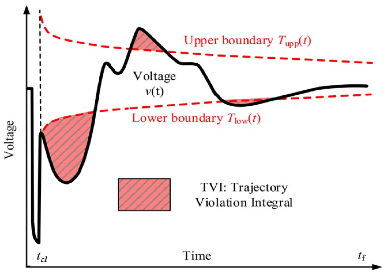
By definition of upper and lower boundaries for post-fault voltage trajectory, the $TVI$ index for each bus in the system is calculated as follows [16]:

$$TVI\left(t\right)={\int }_{t_{cl}}^t{v}_v\left(\tau \right)d\tau$$

(12)

where $v_v\left(t\right)$ is:

$$v_v\left(t\right)=\left\{\begin{array}{c}{T}_{low}\left(t\right)-v\left(t\right)\begin{array}{cc}& \begin{array}{cc}& v\left(t\right)<T_{low}\left(t\right)\end{array}\end{array}\\ v\left(t\right)-T_{upp}\left(t\right)\begin{array}{cc}\begin{array}{cc}& \end{array}& v\left(t\right)>T_{upp}\left(t\right)\end{array}\\ 0\begin{array}{cc}\begin{array}{cc}\begin{array}{cc}& \end{array}& \begin{array}{cc}& \end{array}\end{array}& o.w\end{array}\end{array}\right.$$

(13)

$T_{low}$ and $T_{upp}$ are lower and upper boundaries, respectively, and $T_{low}$ is described by an expression in (14).

$$T_{low}\left(t\right)=\frac{{(\frac{t}{t_f}.e^{\frac{1}{t_f}})}^B}{e^B}.v_{st}\begin{array}{cc}\begin{array}{cc}\begin{array}{cc}& \end{array}& \end{array}& \forall t\in [t_{cl},t_f]\end{array}$$

(14)

In Equation (14), $v_{st}$ is steady state voltage and B is used for calibrating damping of boundaries. In addition $T_{upp}$ is calculated using (15).

$$T_{upp}\left(t\right)=2-T_{low}\left(t\right)$$

(15)

Figure 1 illustrates the $TVI$s concept in which $t_{cl}$ refers to fault clearing time, and $t_f$ is the time that is considered for a short-time voltage stability study. Index $TV{I}_{tot}$ in (16) is used for a system based on the bus indices. In this equation, $v_{v,i}$ is $v_v$ at bus i.

$$TV{I}_{tot}\left(t_f\right)=\frac{1}{n}\sum _{i=1}^n{\int }_{\tau =t_{cl}}^{t_f}{v}_{v,i}d\tau$$

(16)

2.5. Transient Voltage Severity Index ($TVSI$)

There is another index similar to $TVI$ which is used in [17,18] as the voltage index for dynamic VAR planing called the transient voltage severity index ($VSRI$). This index is calculated using (17).

$$TVSI\left(t_f\right)=\frac{{\displaystyle \sum _{i=1}^n}{\displaystyle \sum _{t=t_{cl}}^{t_f}}TVD{I}_{i,t}}{n\times (t_f-t_{cl})}$$

(17)

$TVDI$ is the transient voltage deviation index and calculated by

$$TVD{I}_{i,t}=\left\{\begin{array}{c}\begin{array}{cc}\frac{\left|v_i\left(t\right)-v_{i,0}\right|}{v_{i,0}}\begin{array}{cc}& \end{array}& \frac{\left|v_i\left(t\right)-v_{i,0}\right|}{v_{i,0}}>\mu \end{array}\\ \begin{array}{cc}0& \begin{array}{cc}\begin{array}{cc}& \end{array}& \begin{array}{cc}& o.w\end{array}\end{array}\end{array}\end{array}\right.$$

(18)

The $\mu$ parameter is maximum acceptable voltage deviation and usually is equal to 20%.

2.6. Voltage Stability Risk Index ($VSRI$)

Voltage stability index (VSRI) has been used in [12] as a dynamic voltage stability criterion to assess voltage stability for determining a suitable location for the load curtailment. The index has been considered in [22] as a long-term voltage stability index to identify the vulnerability of the system to the voltage instability at each bus following a contingency. It utilizes the time series data of the bus voltages and does not require any input for other buses.

This index can be computed from time series of the voltages RMS values measured by PMU at systems’ buses. For calculating $VSRI$, let PMU measurements for the voltage of each bus are specified as $y\left(t\right)={[y_1,y_2,\dots ,y_M]}^T$. The following steps are used for $VSRI$ calculation [12,22]:

• The moving average value of the bus voltage at jth instant with taking N initial samples is described by (19).

  $$\left\{\begin{array}{c}\begin{array}{c}{v}_j={\displaystyle \sum _{k=1}^j}{y}_k/\phantom{y_{k}j}j\end{array}\begin{array}{ccc}& ,& j=1,2,\cdots ,N\begin{array}{cc}& \end{array}\end{array}\\ v_j={\displaystyle \sum _{k=j-N+1}^j}{y}_k/\phantom{y_{k}N}N\begin{array}{ccc}& ,& j=N+1,\cdots ,M\end{array}\end{array}\right.$$

  (19)
  According to (19), the average $v_j$ is computed by using j samples existing in the data window before filling the window by N initial samples ($j<=N$). When the window is filled by N samples, according to (19), the average $v_j$ is computed on a moving window including N samples from $j-N+1$ till j for $j>N$. The voltage stability is monitored by M measured samples.
• The percentage diversity, $d_j$, at jth instant between $y_j$ and $v_j$ is computed as

  $$d_j=(y_j-v_j)\times 100/\phantom{100v_j}{v}_j\begin{array}{ccc}& ,& j=1,2,\cdots ,M\end{array}$$

  (20)
  In (20), $d_j$ indicates the normalized deviation of the current sample, $y_j$ with respect to the moving average based on $v_j$. Thus, it can reflect the current situation of buses voltage with respect to the average of N past samples. Small (big) $d_j$ means a small (big) deviation respect to the average of past samples.
• By calculating integral of $d_j$ curve and averaging over the N, VSRI is calculated as follows:

  $$\begin{array}{cc}VSR{I}_j=\hfill & {\displaystyle \sum _{k=1}^j}\frac{(d_k+d_{k-1})}{2j}\begin{array}{ccc}& \begin{array}{cc}& \end{array}& \begin{array}{cc}& j\le N\end{array}\end{array}\\ VSR{I}_j=\hfill & {\displaystyle \sum _{k=j-N+1}^j}\frac{(d_k+d_{k-1})}{2N}\begin{array}{cc}& N+1\le j\le M\end{array}\end{array}$$

  (21)

The area under $d_j$ curve indicates the summation of the deviation of the bus voltage with respect to the dynamic average value of it during an interval from the fault clearing time to the final study time. Thus, VSRI models the dynamic behavior of the buses voltage and it can be used to evaluate short-term voltage stability.

After these steps, $VSRI$ for individual buses can be determined. If the buses voltage are stable after disturbance, VSRI of all buses converges to zero. The convergence time depends on load and system characteristics. The buses with the smallest negative VSRI are identified as the most vulnerability to the voltage instability.

For computing the system’s $VSRI$, in the second step, $D_j$ is used instead of $d_j$ in Equation (21). $D_j$ comes from Equation (22) in which $d_{j,i}$ refers to percentage diversity at jth instant ($d_j$) in bus i.

$$D_j=\frac{1}{n}\sum _{i=1}^n{d}_{j,i}$$

(22)

However, to use $VSRI$ in short-term voltage stability monitoring, an algorithm is proposed in Section 3.2.6.

3. Simulation Scenarios

In this section, a number of dynamic simulations carried out on IEEE 39-bus test system are used to create proper scenarios related to short-term voltage stability phenomenas. The obtained data are then used to compute the introduced SVS indices for each scenario. The 39-bus system is a well-known power system in dynamic studies which has 10 generators, 12 transformers, 19 loads, and 34 transmission lines. The load flow and dynamics data for the 39-bus system are available in [23]. The DIgSILENT power factory program is adopted for time-domain dynamic simulations and to generate the required data for testing the proposed indices.

The operating point described in [23] is taken into account as the basic condition of the 39-bus system as shown in

Table A1. Different conditions for creating SVS database using IEEE-39bus system.

Num	Contingency Type	Affected Element	Fault Location	Dynamic Load Proportion	U Coefficient	Stability
1	Fault	Lines 2–3	0%	0%	1	stable
2	Fault	Lines 2–3	100%	0%	1	stable
3	Fault	Lines 2–3	100%	30%	1	stable
4	Fault	Lines 2–3	100%	30%	0.9	stable
5	Fault	Lines 2–3	100%	60%	0.9	unstable
6	Fault	Lines 2–3	100%	0%	1.2	stable
7	Fault	Lines 4–14	0%	60%	0.8	stable
8	Fault	Lines 4–14	0%	80%	0.8	stable
9	Fault	Lines 4–14	0%	50%	1.2	unstable
10	Fault	Lines 4–14	50%	30%	1	stable
11	Fault	Lines 4–14	50%	70%	1.1	unstable
12	Fault	Lines 4–14	50%	30%	1.2	stable
13	Fault	Lines 4–14	100%	70%	1.1	unstable
14	Fault	Lines 4–14	100%	0%	0.8	stable
15	Fault	Lines 4–14	100%	60%	0.8	stable
16	Fault	Lines 4–14	100%	80%	0.8	stable
17	Fault	Lines 4–14	100%	0%	1.2	stable
18	Fault	Lines 4–14	100%	30%	1.2	stable
19	Fault	Lines 21–22	0%	0%	1.2	unstable
20	Fault	Lines 21–22	0%	0%	1	stable
21	Fault	Lines 21–22	0%	30%	0.8	stable
22	Fault	Lines 21–22	50%	15%	1	unstable
23	Fault	Lines 21–22	50%	10%	1	stable
24	Fault	Lines 21–22	100%	10%	1	unstable
25	Fault	Lines 21–22	100%	5%	1	stable
26	Fault	Lines 21–22	100%	30%	0.8	stable
27	Fault	Lines 21–22	100%	30%	0.9	stable
28	Fault	Lines 21–22	100%	45%	0.9	unstable
29	Fault	Lines 16–19	0%	0%	1	stable
30	Fault	Lines 16–19	20%	30%	1	stable
31	Fault	Lines 16–19	30%	0%	1.1	stable
32	Fault	Lines 16–19	31%	80%	0.8	unstable
33	Fault	Lines 16–19	35%	0%	1.1	stable
34	Fault	Lines 16–19	50%	30%	1	stable
35	Fault	Lines 16–19	50%	80%	0.8	stable
36	Fault	Lines 16–19	100%	80%	0.8	stable
37	Fault	Lines 16–19	22%	0%	1.1	stable
38	Fault	Lines 17–27	0%	60%	1	unstable
39	Fault	Lines 17–27	0%	65%	1	unstable
40	Fault	Lines 17–27	0%	0%	1	stable
41	Fault	Lines 17–27	0%	80%	0.8	unstable
42	Fault	Lines 17–27	0%	30%	1	stable
43	Fault	Lines 17–27	0%	60%	0.9	stable
44	Fault	Lines 17–27	50%	0%	1	stable
45	Fault	Lines 17–27	50%	30%	0.9	stable
46	Fault	Lines 17–27	50%	60%	0.9	stable
47	Fault	Lines 17–27	100%	0%	1	stable
48	Fault	Lines 17–27	100%	50%	1	unstable
49	Fault	Lines 17–27	100%	45%	1	stable
50	Fault	Lines 17–27	100%	30%	0.9	stable
51	Fault	Lines 17–27	100%	70%	0.9	unstable
52	Fault	Lines 17–27	100%	0%	1.1	stable
53	Fault	Lines 22–23	50%	30%	1.1	stable
54	Fault	Lines 22–23	50%	45%	1.1	stable
55	Fault	Lines 22–23	50%	50%	1.1	unstable
56	Fault	Lines 23–24	0%	0%	1	stable
57	Fault	Lines 23–24	50%	0%	1	stable
58	Fault	Lines 23–24	50%	56%	1	unstable
59	Fault	Lines 23–24	100%	0%	1	stable
60	Fault	Lines 23–24	100%	40%	1	stable
61	Fault	Lines 23–24	100%	48%	1	unstable
62	Fault	Lines 23–24	100%	49%	1	unstable
63	Fault	Lines 23–24	100%	50%	1	unstable
64	Fault	Lines 23–24	100%	55%	1	unstable
65	Fault	Lines 28–29	0%	80%	0.8	unstable
66	Fault	Lines 28–29	0%	0%	1.1	unstable
67	Fault	Lines 28–29	100%	70%	0.9	unstable
68	Fault	Lines 28–29	100%	80%	0.9	unstable
69	Fault	Lines 28–29	100%	0%	1.1	unstable
70	Fault	Lines 28–29	100%	30%	1.1	unstable
71	Fault	Bus 1	-	30%	1	stable
72	Fault	Bus 1	-	0%	1.2	stable
73	Fault	Bus 1	-	60%	1.2	stable
74	Fault	Bus 25	-	0%	1	stable
75	Fault	Bus 25	-	30%	1	stable
76	Fault	Bus 25	-	45%	1	stable
77	Fault	Bus 25	-	50%	1	unstable
78	Fault	Bus 25	-	55%	1	unstable
79	Fault	Bus 25	-	0%	1.1	stable
80	Fault	Bus 25	-	30%	1.1	unstable
81	Fault	Bus 25	-	35%	1.1	unstable
82	Fault	Bus 25	-	40%	1.1	unstable
83	Fault	Bus 29	-	60%	1.2	stable
84	Fault	Bus 29	-	75%	1.2	stable
85	Fault	Bus 29	-	80%	1.2	stable
86	Outage	Lines 16–17	-	0%	1	stable
87	Outage	Lines 16–17	-	60%	1	stable
88	Outage	Lines 16–17	-	60%	1.2	stable
89	Outage	Lines 16–19	-	30%	1	stable
90	Outage	Lines 16–19	-	30%	1.2	stable
91	Outage	Lines 16–19	-	80%	1.2	stable
92	Outage	Trans 20–34	-	80%	1.2	stable
93	Outage	Lines 21–22	-	0%	1	stable
94	Outage	Lines 21–22	-	30%	1	stable
95	Outage	Lines 21–22	-	60%	1	stable
96	Outage	Lines 21–22	-	0%	1.2	stable
97	Outage	Lines 21–22	-	25%	1.2	stable
98	Outage	Lines 21–22	-	35%	1.2	unstable
99	Outage	Lines 21–22	-	40%	1.2	unstable
100	Outage	Lines 21–22	-	45%	1.2	unstable

in Appendix A. A complex load model including both dynamic and static models is used for loads modeling in the studied system. In this model, a dynamic part consists of induction motors while a constant impedance model is considered for a static part of the model.

3.1. Scenarios

To achieve comprehensiveness on SVS phenomenas, six different scenarios are considered that are representative of different categories of dynamic transient conditions.

Six scenarios are generated for conditions given below:

(a)

In this case, the power system is considered to be at the basic condition and 70% of loads are set as dynamic loads. A sudden outage of lines 16–17 at time $t=0.2$ s is taken into account for generating the required data.

(b)

Active and reactive powers consumed by loads and generated by generators are adjusted to $90\%$ of the basic condition. Dynamic proportion of loads is taken equal to $20\%$. A three-phase fault at time $t=0.1$ s occurs on lines 16–17 near bus 17 and cleared by the outgoing line at time $t=0.2$ s.

(c)

This case is related to an occurring fault on lines 21–22 near bus 21 at time $t=0.1$ s. Consumed and generated power are $90\%$ of basic condition and a proportion of dynamic loads are set to $45\%$. Fault is cleared at time $t=0.2$ s.

(d)

This scenario is similar to (b), but the load’s dynamic part is increased to $45\%$.

(e)

This scenario is similar to (c), but active and reactive power of loads and generators are increased to $110\%$ of their amount in basic condition, and the dynamic part of loads is increased to $50\%$.

(f)

A sudden outage of lines 21–22 is taken into account at time $t=0.2$ s. The consumed and generated power of loads and generators are adjusted at $120\%$ of the basic operating point while a dynamic part of loads is equal to $60\%$.

By simulating these scenarios on a 39-bus IEEE test system, the variation of voltage magnitude at buses 6, 8, 14, 16, 21, and 27 are shown in Figure 2. As shown in this figure, this scenario includes three stable and three unstable cases from the perspective of SVS. In case (a), voltage stability is maintained without any sag and swell. Although in cases (b) and (c) voltage stability is maintained, voltage sage and swell are observed. Case (c) is related to a significant voltage dip. In cases (d), (e), and (f), voltage magnitude in buses drops after outgoing faulty line at time $t_{cl}=0.2$ s, and this condition has led to short-term voltage instability. Although these three cases are related to instability, but time and pattern of voltage magnitude falling and oscillation are different.

3.2. SVS Indices Implementation

In this section, indices that are presented in Section 2 are used to SVS assessment for the defined scenarios in the previous section. In the online voltage stability monitoring, the time series of voltage magnitude at system buses are built using PMU measurement. The number of installed PMUs in power system are limited in practice due to some factors such as existing communication infrastructure big data and economic issues. If power system is observable, with an $n_{pmu}$ PMU device, voltage variation in all system buses can be obtained by state estimation techniques [24]. However, in unobservable systems, voltage time series can be obtained only in the buses with PMU, so SVS monitoring can be highly affected. It has been assumed that just voltage of buses 5, 6, 7, 8, 12, 14, 15, 16, 17, 21, 24, and 27 are available as time series. These time series include buses voltage magnitude after fault clearing time ($t_{cl}$).

In WAMS, PMUs send data with sampling rates in the range of 0.5–4 per cycle to the monitoring center. In the simulation, PMU data with sampling rate 2 per cycle is used to mimic the practical cases. The considered time for short-term voltage stability analysis is 1–2 s. Therefore, the time of 2 s is considered for our calculations. Simulations are performed using MATLAB codes and indices are calculated for scenarios. Then, by analyzing results, an instruction for short-term voltage instability assessment by each index is suggested.

3.2.1. LE

For use of $LE$ for SVS assessment, we need to take N initial samples. By taking N as equal to 30, the system LE evolutions for defined scenarios have been computed until time 2 s and shown in Figure 3.

We expect LEs to have a negative amount for stable states and positive in unstable cases. As shown in Figure 3, for unstable states (d, e, f), LEs are positive. However, in stable cases (a, b, c), LEs evolution oscillates between negative and positive amounts. This problem can be solved with choosing different parameters like increasing time interval or taking more initial samples. With applying phase rectification (PR), which is proposed in [13], LE accuracy dependence on parameter setting will disappear. However, in this paper, we focus on SVS monitoring with simple computing indices and in time less than 2 s. Then, without using PR, we try to propose an instruction which can separate stable and unstable cases by $LE$.

As expected, at unstable cases, LEs are positive in most of the considered time intervals. In the case (c), which implies a critical stable case with noticeable voltage sag, LEs take positive and negative amounts frequently. Case (b) shows stable conditions without significant voltage sag. LEs take positive amounts only in some time instances, while they have a negative amount at most of the considered time. Hence, it can be concluded that LE evolution for stable/unstable cases are mostly negative/positive in time intervals less than 2 s. Case (a), which is related to stable condition and voltage magnitude after disturbance, has insensible fluctuation, and LE evolution isn’t mostly negative or positive. This problem can be fixed with taking a bigger amount for N. Figure 4 depicts LEs evolution in case (a) for $N=60$. As shown in this figure, LEs are negative in most of time interval.

From these results, instructions for SVS monitoring by Lyapunov exponents are proposed as follows:

• The number of initial samples should be appropriate, for example taken equal to 60.
• When LE’s evolution are mostly negative in certain intervals, it implies a stable state.
• If LE’s evolution in a considered interval is mostly positive, it indicates short-term voltage instability.
• If LE’s evolution isn’t mostly negative or positive, it represents a critical status with significant voltage variation.

However, it is noted that the method based on LE should be enhanced with more modifications to guarantee correct work for all cases.

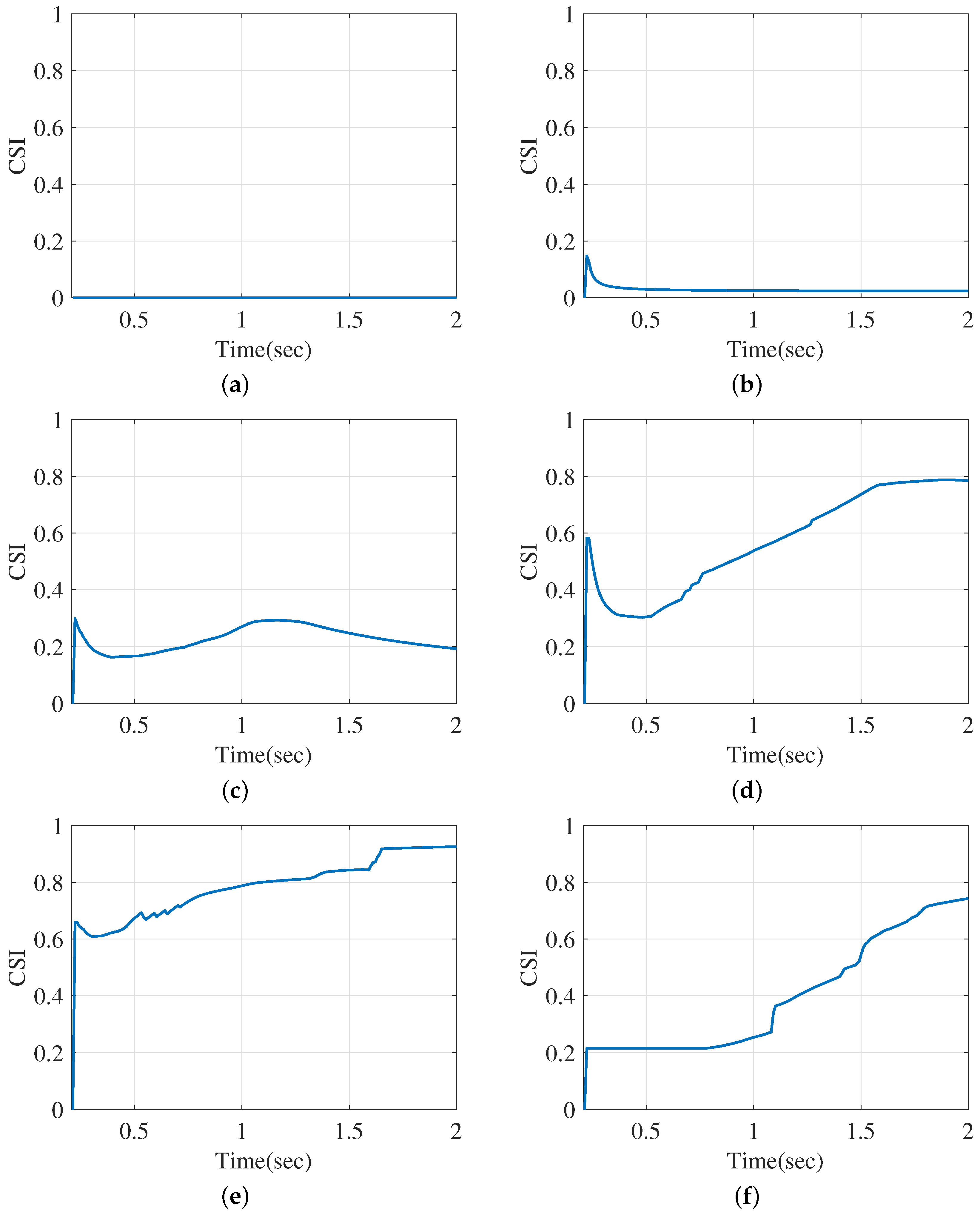
3.2.2. CSI

In six defined scenarios, $S{I}_v$s and $S{I}_t$s are computed for selected buses and $CSI$ for different time intervals are obtained where the results are shown in Figure 5. It is obvious from Equations (3)–(6) that, in unstable cases, $S{I}_v$s and $S{I}_t$s for system buses are near one and then for $CSI$.

For cases in which voltage variation is in the range acceptable and voltage magnitude is higher than 0.8 pu in the time interval, $S{I}_v$ and $S{I}_t$ for buses are equal to zero. In contrast, if the voltage dip exceeds 0.2 pu, the values’ range of $S{I}_v$s and $S{I}_t$s is $[0,1]$. Thus, if $CSI$ has a value more than zero, then voltage magnitude has significant variations.

According to Figure 5, for instability detection, it can be said that, when $CSI$ is more than a certain threshold like 0.6 pu after 2 s from clearing time, the occurred case is an unstable condition. For times less than $1.5$ s, threshold can be reduced to 0.5 pu.

3.2.3. $PI$

Similar to $CSI$, after calculating $P{I}_v$, $P{I}_t$, and $P{I}_{vmax}$, the system’s $PI$ index is calculated for six defined conditions. Figure 6 shows $PI$ amounts calculated in different time intervals. The maximum acceptable voltage dip and its time continuance are taken equal to $\Delta v_{max}=0.2$ pu and ${\tau }_{max}=20$ cycle. As shown in Figure 6, unstable cases have a big amount for a $PI$ index. In these cases, the $PI$ take amounts in order of 1000 or more. The $PI$ for stable cases varied from zero to 1000. According to Figure 6c, in critical stable conditions $PI$ could be near 1000.

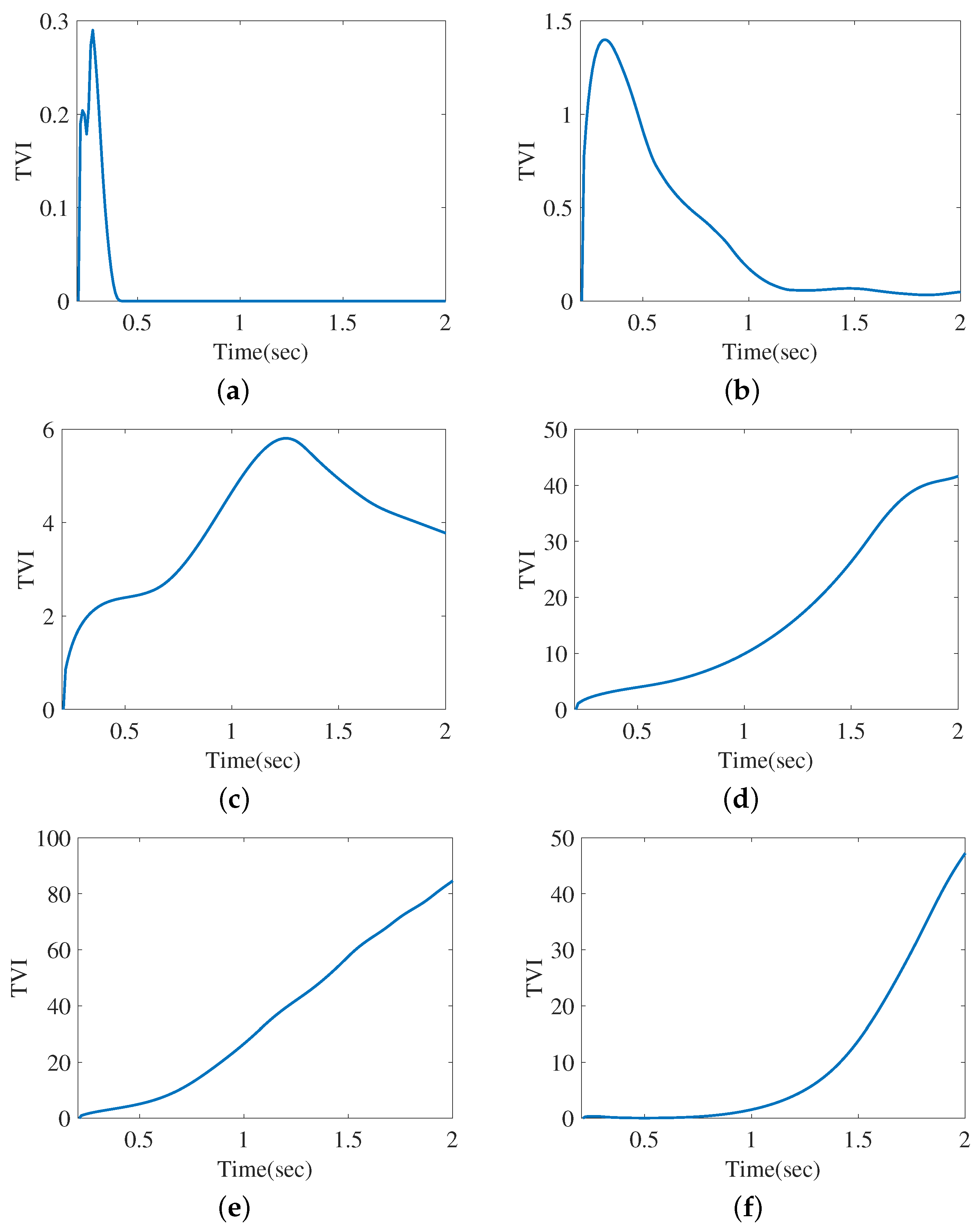
3.2.4. TVI

As mentioned in Section 2.4, $TVI$ is an index that calculates voltage variation from determined boundaries. In Equation (14), parameters are set to their standard amounts in [16]. Thus, parameters B and $v_{st}$ are taken to be equal to 0.05 and 0.9, respectively. Then, $TV{I}_{tot}$ is calculated for six defined scenarios and results are presented in Figure 7.

It is obvious from Figure 7 that, in stable status, $TVI$ is close to zero and, in unstable conditions, $TVI$ take amounts more than zero. Because $TVI$s take different numbers according to system type, using $TVI$ in SVS monitoring needs to determine corresponding thresholds. In our study cases, in a time interval of 2 s, $TVI$ more than 10 is related to voltage instability, and we can say definitely that $TVI$ would be increased with passing time in unstable conditions.

3.2.5. TVSI

According to the $TVSI$ formula, we expect $TVSI$ to have a higher amount in unstable cases. Figure 8 shows variations of $TVSI$ in six defined scenarios for different time intervals. The $TVSI$ in small time intervals of the $t_{cl}$ has a high amount. In some cases, $TVSI$ should be used after a certain time, for example 0.5 after the $t_{cl}$ to detect instability.

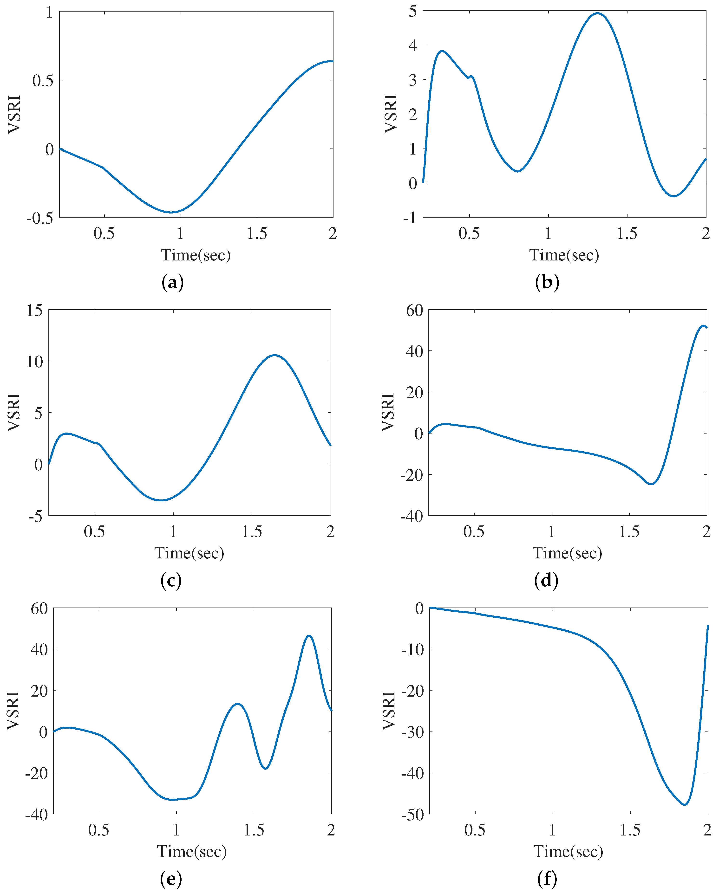
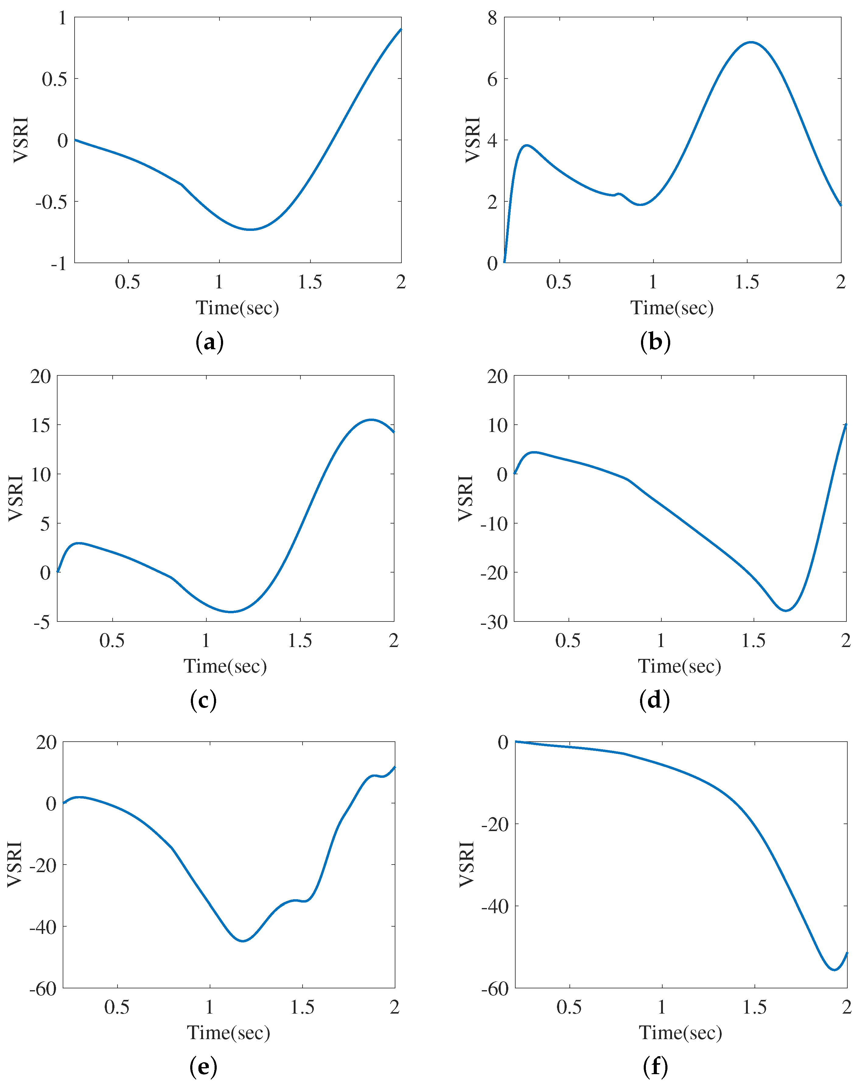
3.2.6. VSRI

Index $VSRI$ is used in this paper for SVS monitoring. By taking a number of initial samples equal to 30 ($N=30$), $VSRI$ has been calculated for six scenarios according to Figure 9. As shown in this figure, in unstable conditions, $VSRI$ is mostly negative and its variation range in a time interval equal to 2 s is more than 20 pu. Based on these figures, for SVS monitoring using $VSRI$, an instruction is proposed as follows:

• If the minimum of $VSRI$ is less than $-20$, the state implies an unstable condition.
• If $VSRI$ varies more than $2pu$ in a selected interval, and the absolute amount of minimum $VSRI$ is higher than the maximum of $VSRI$, the condition is unstable.
• Otherwise, the index VSRI is associated with the stable conditions.

Using this instruction, we can separate stable and unstable conditions from each other. Notice that this instruction is provided for instability detection in a time interval equal to 2 s with $N=30$.

For studying the effect of parameters setting in SVS assessment using $VSRI$, we repeat calculations by taking N equal to 60. Results are shown in Figure 10. It is obvious that the effect of increasing initial samples on SVS assessment using $VSRI$ isn’t considerable and introduced instruction is very applicable even in a time of less than $1.5$ s.

4. Comparison and Results

In order to compare the modified and proposed indices in this paper, the reliability and speed of different indices in SVS assessment are evaluated. For this purpose, a database of simulation data for many scenarios has been provided based on the basic operating point mentioned in [23], considering different disturbances, fault locations, portion of dynamic loads, and taking different consumed and generated power by loads and generators.

The scenarios include 100 cases, where there are 66 stable and 34 unstable cases. The modified and proposed indices and their corresponding suggested instructions have been applied to determine unstable cases from an SVS point of view. With taking a different time interval from 0.8 s to 2 s, the performance of each of the six mentioned indices in SVS monitoring are provided in

Table 1. SVS indices performance in instability detection.

Time Interval (sec)	Index Error in Instability Detection (%)
	LE	CSI	PI	TVI	TVSI	VSRI
0.8	15	15	25	29	23	7
1	35	12	17	25	19	3
1.2	40	9	11	24	17	6
1.5	36	6	6	12	14	4
2	10	6	4	7	12	4

using computation of their total error in instability detection. As shown in Table 1, using the Lyapunov exponent without phase rectification in SVS monitoring is not reliable in time 2 s. The $CSI$ and $TVI$ indices have average performance in SVS monitoring. They need at least 2 s for instability detection. $VSRI$’s error at short-term voltage instability detection is minimal and near $3\%$. Furthermore, SVS monitoring using $VSRI$ needs 1 s for detecting instability. This research shows that the proposed $VSRI$ has the best performance between the available and modified indices for short-term voltage stability monitoring.

A further detailed comparison study between the modified and proposed indices considering the number of unstable cases detected as stable cases and conversely the stable cases detected as unstable cases is introduced in

Table 2. SVS indices performance in instability detection.

Index name	Time Interval (sec)	Index Total Error in SVS Assessment (%)	Number of Unstable Cases Detected as Stable Cases	Number of Stable Cases Detected as Unstable Cases
LE	0.8	15	6	9
	1	35	3	32
	1.2	40	3	37
	1.5	36	3	33
	2	10	1	9
CSI	0.8	15	15	0
	1	12	12	0
	1.2	9	9	0
	1.5	6	6	0
	2	6	6	0
PI	0.8	25	25	0
	1	17	17	0
	1.2	11	11	0
	1.5	6	6	0
	2	4	4	0
TVI	0.8	29	17	12
	1	25	12	13
	1.2	24	9	15
	1.5	12	0	12
	2	7	0	7
TVSI	0.8	23	23	0
	1	19	16	3
	1.2	17	11	6
	1.5	14	3	11
	2	12	3	9
VSRI	0.8	7	2	5
	1	3	0	3
	1.2	6	1	5
	1.5	4	2	2
	2	4	2	2

. It is worth mentioning that the ability to correctly detect unstable cases is more important compared to the detection stable cases. As presented in Table 2, LE’s accuracy in instability detection for time intervals less than 2 s is not appropriate. Although the error is mostly because of detecting stable cases as unstable cases, there is a significant number of stable cases which are detected as unstable cases and cause incorrect operation of control systems.

The comparison results clearly show that, by increasing the time interval, LE index performance can be enhanced, and it has acceptable performance if the time is set to 2 s. However, such time interval is long especially for online SVS monitoring, which identifies an LE index as an unsuitable index for online SVS monitoring applications. Likewise, the detailed performance of CSI in SVS assessment is inserted in Table 2. As expected by an increasing time interval, the performance of CSI in SVS assessment has been improved. It can be seen from the table that total detection error in CSI has been decreased from $15\%$ in time $0.8$ s to $6\%$ in time $1.5$ s. The total error of this index in SVS assessment is generally due to unstable cases detected as stable cases. Although the CSI’s total error is lower than LE, it is much worse than LE because it has worse performance in detecting the unstable cases which are very important to the power system operators.

According to Table 2, PI ability in the detection of the short-term voltage instability is similar to CSI, and PI’s detection total error is related to bad operation in terms of detecting unstable cases as stable cases. However, CSI’s error in time intervals less than 1 s is lower than PI, but PI has slightly better performance with time intervals equal to 2 s.

The TVI index performance in SVS assessment has also been shown in Table 2. It can be seen that TVI’s total error is decreased from $29\%$ in time $0.8$ s to $7\%$ in time 2 s and unstable cases’ misdiagnosis is equal to zero with time intervals more than $1.5$ s. Therefore, it can be identified that TVI has proper performance in SVS monitoring for time intervals close to $1.5$ s. However, the main practical problem is related to the high amount of time needed for detecting the unstable cases, which limits its practicability.

Based on the results introduced in Table 2, TVSI has an average performance in SVS assessment. However, TVSI error is mostly related to mistaken detection of stable cases as unstable cases, but, due to the number of misdiagnosed cases, this index is not suitable for SVS online monitoring.

It is obvious from results presented in Table 2 that the proposed VSRI has proper performance and good ability for online SVS assessment. The VSRI total error in instability detection considering a time interval equal to 0.8 sec is less than 10% and most of this error is related to stable cases detected as unstable cases, which makes this index a proper one for practical implementations. For time intervals between 1.5 sec to 2 sec, the VSRI error has been reduced to less than 5% and only two misdiagnosed unstable cases exist. Therefore, it can be concluded that the proposed VSRI is a proper index for SVS online monitoring in modern power systems.

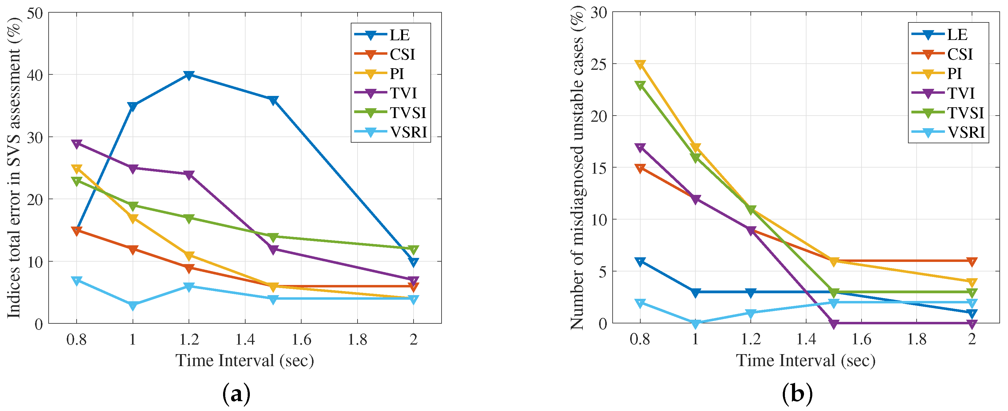
To make clear comparison between the performance of the modified and the six indices in SVS assessment proposed, linear approximation of their total error in instability detection and their accuracy in unstable cases assessment for different time intervals from $0.8$ s to 2 s are depicted in Figure 11a,b, respectively.

As shown in these figures, using LE, CSI, PI, and TVSI in SVS monitoring is not reliable for time 2 s. The $TVI$ index has an average performance in SVS monitoring. It needs at least $1.5$ s for correct unstable cases detection.

The $VSRI$’s error at short-term voltage instability detection is minimum and near $3\%$ as shown in Figure 11b. Furthermore, SVS monitoring using $VSRI$ can be done with time equal to or less than 1 s for detection of instability, which makes this index superior in comparison to others. This research shows that $VSRI$ has better performance in online SVS monitoring compared to the other indices.

As an in-depth comparison between the introduced and modified indices in this paper, a qualitative comparative study is introduced in

Table 3. Summary of index performance in SVS assessment.

Index	LE	CSI	PI	TVI	TVSI	VSRI
Dependence on Threshold	✓	✗	✗	✗	✗	✓
Reliability in times less than 2sec	✗	✓	✓	✗	✗✗	✓✓
Reliability in unstable cases detection	✓	✗✗	✗✗	✓✓	✗	✓✓
Useful in SVS on-line monitoring	✓	✓	✓	✓	✗	✓✓

✓: good, ✗: bad, ✓✓: very good, ✗✗: very bad.

. It is clear that all the introduced indices except the proposed one highly depends on the initial values used for running their algorithms. Such feature makes the $VSRI$ more practical and easy to implement the index in reality. Furthermore, the proposed $VSRI$ index requires less time and has better performance in detecting the unstable cases. Moreover, the proposed index is very suitable for online SVS monitoring applications compared to other indices.

5. Conclusions

In this paper, six indices of voltage stability are analyzed for online SVS monitoring including (i) Lyapunov exponent in the basic form, (ii) contingency severity index, (iii) Potential index, (iv) trajectory violation integral, and (v) voltage severity risk index. Furthermore, using six disturbance scenarios related to different short-term voltage transients in a 39-bus system, their corresponding instructions are proposed. Except Lyapunov exponents which are extensively used in literature, other indices defined in this paper have not been used in SVS monitoring until now, so this paper proposes and modifies them along with appropriate algorithms for the successful use in SVS monitoring in modern power systems. These suggested algorithms are related to a 39-bus test system and could be changed for another one easily. For studying the reliability and speed of these indices with proposed instructions, a clustered database has been generated, and a total error of these methods at instability detection has been calculated. The results show that the simply computed indices that are proposed in this paper are reliable indices for SVS monitoring with detection time near 2 s. The paper proposes a novel index, i.e., VSRI, for online SVS monitoring in modern power systems. For the proposed VSRI, the detection time is less than 1 sec, and its error in detection is less than other indices.