Development of a Prediction Model for Tractor Axle Torque during Tillage Operation

Abstract

In general, the tractor axle torque is used as an indicator for making various decisions when engineers perform transmission fatigue life analysis, optimal design, and accelerated life testing. Since the existing axle torque measurement method requires an expensive torque sensor, an alternative method is required. Therefore, the aim of this study is to develop a prediction model for the tractor axle torque during tillage operation that can replace expensive axle torque sensors. A prediction model was proposed through regression analysis using key variables affecting the tractor axle torque. The engine torque, engine speed, tillage depth, slip ratio, and travel speed were selected as explanatory variables. In order to collect explanatory and dependent variable data, a load measurement system was developed, and a field experiment was performed on moldboard plow tillage using a tractor with a load measurement system. A total of eight axle torque prediction regression models were proposed using the measured calibration dataset. The adjusted coefficient of determination (R²) of the proposed regression model showed a range of 0.271 to 0.925. Among them, the prediction model E showed an adjusted R² of 0.925. All of the prediction models were verified using a validation set. All of the axle torque prediction models showed an mean absolute percentage error (MAPE) of less than 2.8%. In particular, Model E, adopting engine torque, engine speed, and travel speed as variables, and Model H, adopting engine torque, tillage depth and travel speed as variables, showed MAPEs of 1.19 and 1.30%, respectively. Therefore, it was found that the proposed prediction models are applicable to actual axle torque prediction.

1. Introduction

The axle torque of a tractor is used as an indicator for designers to make major decisions, and it can be used for optimal transmission design, transmission failure diagnosis, dynamometer-based fatigue life evaluation, etc. Generally, the axle torque of a tractor differs according to the various conditions such as the soil environment, gear stage, and working type [1,2]. Amongst previous studies, there are some studies on axle torque measurement according to the attached implement [3,4], working speed [5,6,7], tillage depth [6,8], and soil conditions [9,10,11]. However, in order to measure axle torque, a telemetry system that allows for the twisting of a line is required, because the axle rotates, which is very expensive. Thus, as an alternative solution to this problem, the prediction model of tractor axle torque can be used.

There have been studies that have taken various approaches to the prediction of axle torque. According to some studies, axle torque can be predicted using traction force and tire specifications [12,13,14,15]. Zoz and Grisso [14] reported that axle torque can be calculated using the gross traction (GT) and radius of the wheel or tractive device. The GT can be predicted from the model proposed by Brixius [16]. However, since the axle torque during tillage operation is differently affected by various variable conditions, such as slip due to the interaction between the drive wheel and the soil, it is difficult to calculate directly using the traction force. Some researchers have used an artificial neural network (ANN) to predict engine torque [17]. Bietresato et al. [18] proposed an ANN-based prediction method using exhaust gas temperature and engine speed to evaluate engine performance, such as torque and brake specific fuel consumption (BSFC). Rajabi-Vandechali et al. [19] developed a low-cost sensor (engine speed, fuel mass flow, and exhaust gas temperature) and soft computing-based prediction models to estimate engine torque. As a result, it was reported that the coefficient of determination (R²) of the prediction model was 0.99, which means that it could replace the existing expensive method. However, such a prediction model using an artificial neural network has difficulty finding the optimal value of a parameter in a learning process, and problems, such as overfitting, may occur. Therefore, artificial intelligence is mainly used for solving nonlinear problems and need not necessarily be used for solving linear problems. Linear regression analysis can be a good alternative to the methods presented above. Linear regression models have been proposed in various research fields and are used to select explanatory variables that are highly related to actual dependent variables and to develop prediction models [20,21,22]. In the field of tractors, there have been many studies using linear regression models to predict tractor traction performance [23,24,25] and fuel efficiency [26]. Kheiralla et al. [25] performed regression analysis on the traction force of a moldboard plow, disk plow, disk harrow, and rotary tiller using the travel speed, tillage depth, and rotor speed as the main variables. Upadhyay and Raheman [27] proposed a specific draft prediction model of a disk harrow using multiple regression analysis based on front gang angle, cone index, tillage depth, and travel speed. The literature review revealed that multiple linear regression-based approaches for predicting axle torque during tillage are rare, and most of them focus on the prediction of traction force.

In order to use regression analysis to develop a prediction model for a tractor axle model, it is important to select tractor axle torque and key variables that are meaningful and easy to measure. The engine is a power source for the driving axle torque, and representative major data of the engine load, such as engine torque and speed, are closely related to axle torque. To date, most studies have been carried out on tractors equipped with mechanical engines. However, recent tractors have been equipped with electronic engines capable of controller area networks (CAN) communication to respond to Tier-4 environmental regulations. Thus, various types of engine information, including engine torque and speed during field operation, can be measured through CAN, without an additional sensor. Some studies have evaluated a tractor’s load condition based on the fuel rate, engine speed, and percent torque data, measured via CAN [28]. Engine load data have difficulty predicting axle torque directly due to the power loss in hydraulic and electrical systems, depending on the working conditions [13], but since there is a significant correlation between engine load and axle torque, engine load can be used as a main variable for predicting axle torque. Tillage depth and travel speed are the main variables used in the model for predicting the required draft of the proposed major tillage tools from American Society of Agricultural and Biological Engineers (ASABE) and are expected to be closely related to axle torque [6,29]. In addition, slip has been used as a key variable in predicting tractor traction in many studies [16,20,30,31], and some studies have shown that the slip ratio actually affects the axle torque during tillage operation [32]. Therefore, developing a regression model using variables that can affect various axle loads, including measurable variables in the engine, can be a good method for estimating axle torque.

In conclusion, axle torque is one of the most important parameters of tractor transmission, which needs to be continuously predicted during operation. In this study, a low-cost sensor-based prediction model that does not require the installation of an expensive wheel torque transducer of the telemetry type, which is the main advantage of using multiple linear regression, is proposed. The accurate estimation of the output axle torque exerted by attached implements through a low-cost sensor can be used for various technologies for managing tractors during field operations.

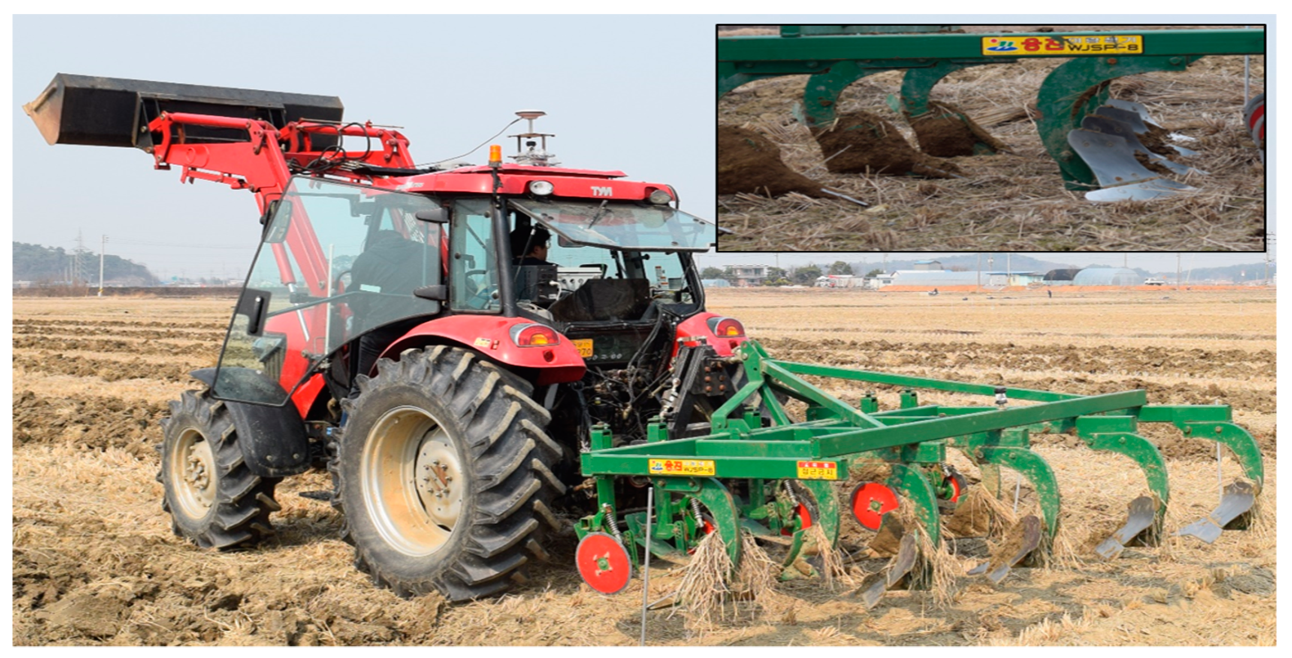
The aim of this study was to develop a prediction model for estimating axle torque by substituting an expensive axle torque sensor, using data on variables that are relatively easy to measure, with a low-cost sensor. Axle torque could be used as an important decision indicator for the optimum design, service life evaluation, and traction performance analysis of transmissions through the prediction model developed in this study. To develop and verify the model, field data were measured through moldboard plow tillage operations. The prediction model was developed based on measured variables using multiple regression. The developed model was verified using the measured actual axle torque from a field experiment.

2. Materials and Methods

2.1. Tractor Power Transmission System

The power transmission system of a tractor transmits the power of the engine to the wheel, with a suitable speed and torque combination, through a gear ratio application at a set gear stage [33]. The tractor transmission consists of a forward and reverse gear, high/low gear, driving shift gear, range shift gear, and spiral bevel gear set, as shown in Figure 1 [34]. Depending on whether two-wheel drive or four-wheel drive is set, the meshing gear is operated, and in the case of four-wheel drive, the meshing gear is engaged, and power is transmitted to the front wheel. The output torque of the gearbox is diverted to the front and rear axles through the meshing gear. Therefore, in order to predict the axle torque to be applied in the design of the transmission, the output axle of the gearbox was selected as the prediction target.

2.2. Field Experiment and Data Measurement

2.2.1. Sensor System

To measure the field data, a 78 kW class tractor (S07, TYM Co., Ltd., Gongju, Korea), which is widely used in Korea, was used in this study. The dimensions of the tractor are 4225 × 2140 × 2830 mm (length × width × height), and the weight is 3985 kg. The rated engine torque at a rated speed of 2300 rpm is 324 Nm.

Figure 2 shows the tractor and load measurement system. The tractor is equipped with an engine (D34P, Doosan Infracore Co., Ltd., Seoul, Korea) capable of CAN communication. The major parameters of the engine are communicated from the engine control unit (ECU) via CANbus J1939 communication. Among them, CAN message data, including engine torque and engine speed, were measured during a field experiment with an accuracy of 1.0%. The tillage depth was calculated through a potentiometer, with an accuracy of 0.1%, built into the lift arm of the three-point hitch. The output value of the potentiometer was calibrated through 10 repeated measurements, and it showed an R² of 0.99 (Tillage depth = −0.2342 × potentiometer value + 32.857). The travel speed was measured using GPS (18 × 5 Hz, Garmin, Olathe, KS, USA) with an accuracy of 5.0%, and the wheel rotational speed was measured using a proximity sensor (Autonics, PRDCMT30-25DO, Seoul, Korea) with hysteresis of the maximum 10% of sensing distance by installing a separate gear jig between the axle case and the wheel. The axle torque was measured using two front torquemeters (Manner Sensortelemetrie GmbH, MW 15 kNm Fu PCM16, Spaichingen, Germany) and two rear torquemeters (Manner Sensortelemetrie GmbH, MW 30 kNm Fu PCM16, Spaichingen, Germany). The linearity deviation of torquemeters is 0.2%. A data acquisition system (IMC, CRONOS compact CRC-400-11, Berlin, Germany) was used to measure field data from each sensor data.

2.2.2. Field Experiment

An experiment was conducted to measure both the sensor data for the prediction model development and the axle torque for model verification, as shown in Figure 3. The location of the experimental field site is Geumam-ri, Dangjin-si 674-10 (36°55′48.1″ N, 126°38′00.3″ E). In this study, an eight-row moldboard plow, which is typically used in Korea, was selected, as shown in

Table 1. Specifications of the moldboard plow used in this study.

Model	Width × Length × Height	Weight	Applicable Power Range	Furrow
WJSP-8	280 × 215 × 125 cm	790 kg	60–90 kW	8

[8].

Table 2. Operating conditions of the tractor, and soil environmental conditions of the field site.

Travel Speed	Tillage Depth	Soil Characteristic
		Texture	Penetration Resistance	Moisture Content
7.09 km/h	15–20 cm	Silt loam	1367 kPa	34.17%

shows the operating conditions of the tractor and soil environment of the field experiment site. The driving gear stages and tillage depth were set to M3 Low (7.09 km/h) and 15–20 cm, respectively, during plow tillage [6]. The soil texture, cone index, and soil moisture content of the field experiment site were referenced as representative variables of the soil environmental conditions. Soil samples were collected, taking into account the plow tillage depth (0–20 cm) at ten uniform locations on the field site. The soil texture was analyzed as silt loam (sand: 16%, silt: 62%, and clay: 22%), according to analytical methods, based on the particle distribution of sand, silt, and clay, as defined by the United States Department of Agriculture (USDA). The cone index was measured using a soil penetrometer (SC 900, Spectrum Technologies, Aurora, IL, USA), and the measurement followed the method suggested in the ASABE standard [35,36]. The cone index value for each depth was expressed as the average cone index from 0 to 150 mm. The soil moisture content was measured using a soil moisture sensor (TDR 350, Spectrum Technologies, Aurora, IL, USA). The soil penetration resistance and soil moisture were 1367 kPa and 34.17%, respectively, which are the average values measured at 100 uniform points on the field experiment site.

2.3. Data Processing

The data collected through field operation need to be processed in order to be applied in regression analysis. The slip was calculated using the GPS-based actual speed and proximity sensor-based theoretical speed, as shown in Equation (1) [15]. The target to predict in this study was the output axle of the gearbox. Since it is difficult to directly measure the torque of the gearbox output axle, it was estimated using measured each wheel axle torque in this study. Thus, it is necessary to calculate the torque of the output axle of the gearbox using the data measured on the four axles. The torque of the target axle was calculated by considering the four wheel torques measured in this study, the gear ratio, and the efficiency between the wheel and gearbox output axle, as shown in Equation (2). The number of gear pairs, gear ratio, and efficiency between each wheel of the front and rear wheels and gearbox are shown in

Table 3. Number of gear pairs, gear ratio, and efficiency between each wheel and gearbox.

Parameters	Number of Gear Pairs	Gear Ratio	Efficiency
Front wheel—gearbox output axle	6	15.8	0.941
Rear wheel—gearbox output axle	3	22.2	0.970

.

$$s=\left(\frac{V_0-V_a}{V_0}\right)\times 100(\%)$$

(1)

where $s$ is the slip ratio (%), $V_0$ is the theoretical speed (km/h), and $V_a$ is the travel speed (km/h).

$$T_a=\left(T_{FL}+T_{FR}\right)/(G_f\times {\eta }_f)+\left(T_{RL}+T_{RR}\right)/(G_r\times {\eta }_r)$$

(2)

where $T_a$ is the output axle torque of gearbox (Nm); $T_{FL}$, $T_{FR}$, $T_{RL}$, and $T_{RR}$ are the front left, front right, rear left, and rear right wheel torque (Nm), respectively; $G_f$ is the gear ratio between the front wheel and gearbox output axle; $G_r$ is the gear ratio between the rear wheel and gearbox output axle; ${\eta }_f$ is the efficiency between the front wheel and gearbox output axle (%); and ${\eta }_r$ is the efficiency between the rear wheel and gearbox output axle (%).

2.4. Statistical Descriptions

The data from the calibration set and verification set used in this study were described using some statistical parameters: the mean, maximum, minimum, range, and standard deviation (SD) in the following Equations (3)–(5) [37].

$$Mean=\frac{{{\displaystyle \sum }}_{i=1}^{i=n}{P}_i}{n},$$

(3)

$$Range=P_{max}-P_{min},$$

(4)

$$SD=\frac{\sqrt{{{\displaystyle \sum }}_{i=1}^{i=n} {\left(P_{i }-Mean\right)}^2}}{\mathrm{N}},$$

(5)

where $P_i$ is the ith parameter data, $P_{max}$ is the maximum parameter data, $P_{min}$ is the minimum parameter data, $n$ is the number of data, and $SD$ is the standard deviation.

2.5. Development of Multiple Regression Models

2.5.1. Model Development Procedure

Figure 4 shows the overall procedure for developing and verifying the multiple regression models using the raw data measured in the field. All of the measured raw data were subjected to a data preprocessing process for use in the model development and verification. The entire dataset (100%) was divided into 75% and 25% and used as a calibration set and validation set, respectively. The validation set was selected randomly within the minimum and maximum values of the entire dataset. The calibration data were used in the development of the regression model, and the developed regression model was verified using the validation set.

2.5.2. Variable Selection

For use in the regression models, the variable was selected based on well-known knowledge regarding the tractor power transmission system and the results of some previous studies. The tractor axle is closely related to the engine load because it is driven by power from the engine. The engine’s operating point depends on its speed, which is based on the engine map, and this determines the engine torque. The engine parameters can be collected without a separate sensor when the tractor is equipped with an electronic engine capable of CAN communication, thereby reducing costs. Therefore, the engine speed and engine torque were selected as the parameters of the engine. In addition, variables for predicting axle torque were selected according to previous studies, which mentioned that the parameters of the tillage depth [6,8,38], slip ratio [6,15,39], and travel speed [5,38,40] had significant effects on tractor load. Therefore, in this study, the engine torque, engine speed, tillage depth, slip ratio, and travel speed were selected as the explanatory variables.

2.5.3. Regression Model Development

The dataset used for the regression model was obtained through a field experiment. The data for the selected explanatory variables in this study are not easy to collect under all conditions. The tractor may not be able to communicate with CAN or may not have a built-in potentiometer. Therefore, in this study, the regression model was developed for each function ($f_1$, $f_2$, and $f_3$) and function combination in order to consider the conditions of data collection and the usability of the model. Equation (6), as function of $f_1$, can be used when the tractor is capable of CAN communication; Equation (7), as function of $f_2$, can be used when the potentiometer is built into the tractor; and Equation (8), as function of $f_3$, can be used when an additional sensor is installed to measure the travel speed and wheel speed of the tractor.

$$T_a=f_1 \left(T_e,S_e\right)$$

(6)

where $T_a$ is the axle torque (Nm), $f_1$ is the functions related to the engine parameters, $T_e$ is the engine torque (Nm), and $S_e$ is the engine speed (rpm).

$$T_a=f_2 \left(D_t\right)$$

(7)

where $f_2$ is the measured data from the built-in sensor in the tractor, and $D_t$ is the tillage depth (cm).

$$T_{a }=f_3 \left(S_t, s\right)$$

(8)

where $f_3$ is the data measured by the additional installed sensors, $S_t$ is the travel speed (km/h), and $s$ is the slip ratio (%).

To develop the axle torque prediction model, a simple regression analysis was used for each function relationship ($f_2$) using the enter method, and a multiple regression analysis was performed for the combination of each functional relationship ($f_1$, $f_3$, $f_1+f_2$, $f_1+f_3$, $f_2+f_3$, $f_1+f_2+f_3$) using the stepwise method. Equation (9) is the equation of the input and output variables of the prediction model [41]. Based on Equation (9), the prediction model was developed, with a total of six variable conditions, such as the engine torque, engine speed, travel speed, slip ratio, and tillage depth, using the SPSS 21 software (SPSS Inc., Chicago, IL, USA).

$$T_a=a_0+a_1{x}_1+a_2{x}_2+\cdots a_n{x}_n+\epsilon$$

(9)

where $a_0,a_1,a_2\cdots a_n$ are the coefficients of the multiple regression, $x_1,x_2\cdots x_n$ are the regression model variables, and $\epsilon$ is the error of the model.

To use regression analysis (including multicollinearity, only when using multiple regression), the following basic assumptions must be satisfied:

• Linearity: The relationship between the dependent and explanatory variables should be linear. This can be confirmed through correlation analysis.
• Normality: The residuals must have a normal distribution, regardless of the value of the independent variable. The mean of the regression standardized residuals is zero, and a normal distribution with a constant variance is assumed. The normality of the estimation error can be confirmed through the distribution of the regression-standardized residuals and the P–P plots of the regression-normalized residuals of the expected cumulative probability versus actual cumulative probability.
• Independence: The residuals in the dependent variable measurements should not affect each other. A Durbin–Watson test (D.W) is conducted to confirm the independence of the residuals of each model. In general, D.W has a value of 0 to 4, and the closer this value is to 2, the more the residual independence is guaranteed [42].
• Homoscedasticity: Homoscedasticity indicates that the scatter of the explanatory variable should be the same, regardless of the value of the dependent variable. Homoscedasticity can be confirmed by a scatter plot of the standardized predicted values and standardized residuals.
• Multicollinearity: There should be no multicollinearity between the explanatory variables, since the multicollinearity of the explanatory variables means that they are expressed in a linear relationship between the explanatory variables of the prediction model, and this is used to confirm correlations between the prediction variables when developing a prediction model. The variance inflation factor (VIF) was used to detect the multicollinearity of the prediction model [43]. VIFs are calculated for the coefficients of each model with the SPSS 21 software, when regression analysis is conducted. In the selection of the regression model, the problem of collinearity is diagnosed using tolerance and the variance inflation coefficient (VIF). Tolerance is the reciprocal of VIF. Some previous studies have reported that if the VIF is greater than 10, there is a problem of multicollinearity [44,45]. In this study, the upper limit of the VIF was set to 10, and values less than that were adopted.

2.5.4. Verification of Multiple Regression Models

Several criteria have been used to evaluate the performance of prediction models based on regression analysis [15,39,46]. In this study, to evaluate the predictive ability of the developed model, the statistical parameters between the actual axle torque and the axle torque predicted through the model were calculated according to the following Equations (10)–(13). The statistical parameters such as R², mean absolute percentage error (MAPE), root mean square error (RMSE), and relative deviation (RD) were used as an evaluative indicator of the development of each model.

$$R^2=\frac{{{\displaystyle \sum }}_{i=1}^{i =N} \left(y_i-y_a\right)-{{\displaystyle \sum }}_{i=1}^{i=N} \left(y_i-\widehat{ y_i}\right)}{{{\displaystyle \sum }}_{i=1}^{i=N}\left(y_i-y_a\right)},$$

(10)

$$MAPE=\frac{1}{N}{\displaystyle \sum }_{i=1}^{i=N}\left|\frac{1}{y_i}\left(y_i-\widehat{y_i}\right)\right|\times 100(\%),$$

(11)

$$RMSE=\sqrt{\frac{1}{N}{\displaystyle \sum }_{i=1}^{i=N}{\left(\widehat{y_i}-y_i\right)}^2},$$

(12)

$$RD=\frac{RMSE}{Mean}\times 100,$$

(13)

where $y_a$ is the mean actual axle torque, $y_i$ is the ith actual axle torque, and $\widehat{y_i}$ is the ith predicted axle torque.

3. Results

3.1. Statistical Descriptions

A statistical description of the calibration and validation dataset for each variable is reported in

Table 4. Statistical description of the calibration and validation dataset for each variable used in this study.

	Parameter	Mean	Max.	Min.	Range	SD
Calibration set (n = 375)	$T_a$ (Nm)	1079.60	1202.69	977.87	224.82	46.82
	$T_e$ (Nm)	316.07	392.40	252.34	140.06	23.20
	$S_e$ (rpm)	2265.09	2410.23	1725.71	684.53	112.58
	$D_t$ (cm)	16.82	22.50	13.73	8.77	1.88
	$S_t$ (km/h)	6.07	6.93	5.04	1.89	0.36
	$s$ (%)	13.40	18.00	9.50	8.50	1.93
Validation set (n = 125)	$T_a$ (Nm)	1080.26	1170.26	987.65	182.61	42.38
	$T_e$ (Nm)	314.65	372.62	259.05	113.57	21.14
	$S_e$ (rpm)	2276.65	2407.68	1889.99	517.69	94.25
	$D_t$ (cm)	16.76	21.29	13.94	7.35	1.68
	$S_t$ (km/h)	6.08	6.90	5.24	1.66	0.34
	$s$ (%)	13.40	17.50	9.88	7.63	1.81

. The means of the gearbox output axle torque, engine torque, engine speed, tillage depth, travel speed, and slip ratio in the calibration set were 1079.60 Nm, 316.07 Nm, 2265.09 rpm, 16.82 cm, 6.07 km/h, and 13.40%, respectively. These showed ranges of 977.87–1202.69 Nm, 252.34–392.40 Nm, 1725.71–2410.23 rpm, 13.73–22.50 cm, 5.04–6.93 km/h, and 9.50–18.00%, respectively. The means of the gearbox output axle torque, engine torque, engine speed, tillage depth, travel speed, and slip ratio in the validation set were 1080.26 Nm, 314.65 Nm, 2276.65 rpm, 16.76 cm, 6.08 km/h, and 13.40%, respectively. These showed ranges of 987.65–1170.26 Nm, 259.05–372.62 Nm, 1889.99–2407.68 rpm, 13.94–21.29 cm, 5.24–6.90 km/h, and 9.88–17.50%, respectively.

3.2. Correlation Analysis

To confirm the linearity between the dependent and explanatory variables, correlation analysis was conducted using Pearson correlations based on the data measured in field experiments.

Table 5. Correlation matrix for variables for predicting axle torque.

	Pearson Correlation Coefficient (p-Value)
Variable	${\mathit{T}}_{\mathit{a}}$	${\mathit{T}}_{\mathit{e}}$	${\mathit{S}}_{\mathit{e}}$	${\mathit{D}}_{\mathit{t}}$	${\mathit{S}}_{\mathit{t}}$	$\mathit{s}$
${\mathit{T}}_{\mathit{a}}$	1.000	0.505 ** (0.000)	−0.396 ** (0.000)	0.931 ** (0.000)	−0.688 ** (0.000)	0.897 ** (0.000)
${\mathit{T}}_{\mathit{e}}$		1.000	0.904 ** (0.000)	0.445 ** (0.000)	0.132 ** (0.005)	0.431 ** (0.000)
${\mathit{S}}_{\mathit{e}}$			1.000	−0.355 ** (0.000)	−0.033 (0.261)	−0.320 ** (0.000)
${\mathit{D}}_{\mathit{t}}$				1.000	−0.714 ** (0.000)	0.984 ** (0.000)
${\mathit{S}}_{\mathit{t}}$					1.000	−0.690 ** (0.000)
$\mathit{s}$						1.000

** Significant value at p < 0.01.

shows the results of correlation analysis for the variables used in this study. The gearbox output axle torque, which is a dependent variable, showed a high correlation coefficient in order of the tillage depth (r = 0.931), slip ratio (r = 0.897), travel speed (r = −0.688), engine torque (r = 0.505), and engine speed (r = −0.396). This indicates that these variables are the main factors directly affecting the axle torque. Overall, there was a very significant difference (p < 0.01) for most variables, and there was no significant difference between the travel speed and engine speed (p > 0.01).

3.3. Prediction Model

3.3.1. Development of the Regression Model

Eight regression models were developed through enter and stepwise methods as a combination of each function source using the measured calibration dataset.

Table 6. Regression model for predicting the axle torque of the tractor.

Model	Source	Regression Model	R2	R2 adj	S.E
A	$f_1$	$T_a=1.626{\mathrm{T}}_{\mathrm{e}}+0.138{\mathrm{S}}_{\mathrm{e}}+252.210$	0.275	0.271	39.98
B	$f_2$	$T_a=23.189D_t+689.467$	0.866	0.866	17.16
C	$f_3$	$T_a=19.599s-16.860S_t+919.198$	0.814	0.813	20.26
D	$f_1+f_2$	$T_a=0.419{\mathrm{T}}_{\mathrm{e}}+0.042{\mathrm{S}}_{\mathrm{e}}+21.785D_t+484.555$	0.878	0.877	16.41
E	$f_1+f_3$	$T_a=2.565{\mathrm{T}}_{\mathrm{e}}+0.302{\mathrm{S}}_{\mathrm{e}}-107.497S_t+237.209$	0.926	0.925	12.79
F	$f_2+f_3$	$T_a=22.340D_t-6.175S_t+741.218$	0.867	0.867	17.11
G	$f_1+f_2+f_3$	$T_a=-0.047{\mathrm{S}}_{\mathrm{e}}+20.179D_t-14.662S_t+935.057$	0.876	0.875	16.54
H	$f_1+f_2+f_3$	$T_a=0.580{\mathrm{T}}_{\mathrm{e}}+14.461D_t-40.263S_t+897.125$	0.899	0.899	14.91

shows the developed regression model, R², adjusted R², and standardized error (S.E) for each regression model. The developed eight regression models showed an adjusted R² range of 0.271–0.925, indicating that the actual axle torque can be predicted with an accuracy of about 27.1–92.5%. The adjusted R² of regression model A, which used the engine torque and engine speed as the main variables, was the lowest, at 0.271. This means that the prediction accuracy is somewhat low, because the adjusted R² is less than 0.3. On the other hand, the adjusted R² of Model B, with the tillage depth, and Model C, with the slip ratio, were 0.866 and 0.813, respectively. These results showed that they had a high accuracy compared to regression Model A. In addition, Model B showed the highest accuracy among the prediction models using a single input source. In case of using a combination of each source as a variable, adjusted R² in Models F and E showed lowest (0.867) and highest (0.925), respectively. The S.E was found to be approximately between 12.79 and 39.98 for all the regression models.

An ANOVA analysis—including the degrees of freedom (Df), sum square (SS), mean square (MS), F-value, and p-value for each model—was performed. The results of the ANOVA regression analysis for each model are shown in

Table 7. Results of the analysis of variance (ANOVA) for each prediction regression model.

Model		Df	SS	MS	F-Value	p-Value
A	Regression	2	225,648	112,824	71	0.000
	Residual	372	594,473	1598
	Total	374	820,120
B	Regression	1	710,323	710,323	2413	0.000
	Residual	373	109,797	294
	Total	374	820,120
C	Regression	2	667,470	333,735	813	0.000
	Residual	372	152,651	410
	Total	374	820,120
D	Regression	3	720,217	240,072	892	0.000
	Residual	371	99,903	269
	Total	374	820,120
E	Regression	3	759,415	253,138	1547	0.000
	Residual	371	60,706	164
	Total	374	820,120
F	Regression	2	711,241	355,621	1215	0.000
	Residual	372	108,879	293
	Total	374	820,120
G	Regression	3	718,582	239,527	875	0.000
	Residual	371	101,538	274
	Total	374	820,120
H	Regression	3	737,632	245,877	1106	0.000
	Residual	371	82,488	222
	Total	374	820,120

. Df, SS, and MS were used to calculate the F-value. The F-value, expressing how much more useful prediction by the regression was than prediction by the average, was the highest in Model B (2413), followed by the values in Models E (1547), F (1215), H (1106), D (892), G (875), C (813), and A (71). In all the models, the significance probability was 0.000, and the explanatory variable included in each model significantly explains the axle torque at a significance level of 0.01.

Table 8. Results of the coefficient analysis for each prediction model.

Model	Variable	S.E	β	t	p-Value	Tolerance	VIF
A	Constant	159.556		1.581	0.115
	$T_e$	0.209	0.806	7.794	0.000	0.182	5.485
	$S_e$	0.043	0.333	3.218	0.001	0.182	5.485
B	Constant	7.992		86.274	0.000
	$D_t$	0.472	0.931	49.123	0.000	1.000	1.000
C	Constant	32.052		28.678	0.000
	$s$	0.751	0.807	26.111	0.000	0.524	1.910
	$S_t$	3.998	0.130	−4.218	0.000	0.524	1.910
D	Constant	65.721		7.373	0.000
	$D_t$	0.508	0.874	42.856	0.000	0.789	1.268
	$T_e$	0.090	0.208	4.649	0.000	0.165	6.078
	$S_e$	0.018	0.102	2.383	0.018	0.179	5.573
E	Constant	51.057		4.646	0.000
	$T_e$	0.069	1.271	37.306	0.000	0.172	5.817
	$S_t$	1.882	0.831	−57.115	0.000	0.942	1.062
	$S_e$	0.014	0.726	21.478	0.000	0.175	5.722
F	Constant	30.289		24.471	0.000
	$D_t$	0.672	0.897	33.248	0.000	0.491	2.038
	$S_t$	3.487	0.048	−1.771	0.077	0.491	2.038
G	Constant	47.526		19.675	0.000
	$D_t$	0.772	0.810	26.132	0.000	0.347	2.878
	$S_e$	0.009	0.113	−5.179	0.000	0.707	1.414
	$S_t$	3.749	0.113	−3.911	0.000	0.397	2.519
H	Constant	30.029		29.876	0.000
	$D_t$	0.931	0.580	15.541	0.000	0.194	5.144
	$S_t$	4.362	0.311	−9.231	0.000	0.238	4.197
	$T_e$	0.053	0.288	10.895	0.000	0.389	2.570

shows the analysis results for the regression coefficients of each axle torque prediction model. The β value of the standardized coefficient is an indicator of the influence of the explanatory variable on the dependent variable in each model. The tillage depth was the most used variable, as it was used in five of eight models (Models B, D, F, G, and H). The β of the tillage depth in Models B, D, F, G, and H were 0.931, 0.874, 0.897, 0.810, and 0.580, respectively. In particular, in Models B, D, F, G, and H, the β of the tillage depth was higher than that of the other variables, and this means that the tillage depth had the highest influence on the axle torque prediction. The explanatory variables of Model E with the highest accuracy were engine torque (t = 37.306, p = 0.000), travel speed (t = −57.115, p = 0.000), and engine speed (t = 21.478, p = 0.000). In this model, according to β, it was found that engine torque, travel speed, and engine speed had the high influence, in order. In most cases, the constant and coefficient of the explanatory variable, obtained for each developed axle torque prediction regression model, showed significant differences (p < 0.01), except for the constant (p = 0.115) in Model A, engine speed (p = 0.018) in Model D, and travel speed (p = 0.077) in Model F. Nevertheless, Table 7 shows that the p-values of the regression Models A, D, and F were significantly different (p < 0.01). Thus, Models A, D, and F are considered to be usable.

3.3.2. Normality Test of Residuals

The results of the normality test of the residuals are shown in Figure 5 and Figure 6. Figure 5 shows the distribution of the regression standardized residuals for each prediction model (A–H). It shows the mean of the regression standardized residuals to be zero and a normal distribution with constant variance. As a result, it was confirmed that the residuals in each model satisfactorily follow a normal distribution and satisfy normality. Figure 6 shows the P–P plots of the regression-normalized residuals of the expected cumulative probability versus actual cumulative probability for each regression model (A–H). It can be seen that the plotted values follow a diagonal line and thus show a normal distribution.

3.3.3. Independence

A Durbin–Watson test (D.W) was conducted to confirm the results of the independence test of the residuals for all the regression models, as shown in

Table 9. Results of the Durbin–Watson test for each prediction regression model.

Model	A	B	C	D	E	F	G	H
D.W	1.340	2.113	2.084	2.104	2.077	2.105	2.124	2.146

. The results showed a range of 1.340–2.146 for all the regression models. Among them, Models B–H showed a D.W value close to 2, which means that they guarantee the independence of the residuals. Model A shows a D.W value of less than 1.5, which means that it may have difficulty guaranteeing the independence of the residuals.

3.3.4. Homoscedasticity

Figure 7 shows that the residual plot is rectangular in all the axle torque prediction models, and a number of points are distributed around the center. The plots of all the regression models indicate that the residuals are all unbiased and homoscedastic, because there was no pattern. According to the information presented in a previous study, if the residual has a mean value of 0 in the thin vertical strip and the spread of the residual is the same in the thin vertical strip, the standard deviation is the same all across the plot [47]. Since the results of this study are similar, the residual mean is 0, and the standard deviation can be said to be the same across the plot in all the regression models.

3.3.5. Multicollinearity

The collinearity problems of the developed linear regression models were evaluated using the tolerances and VIFs. Table 8 shows the tolerance and VIF of each model. All the regression models showed a VIF of less than 7 for all the variables, and the highest tolerance was 6.078 for the engine torque variable in Model D. For all variables, the VIF is less than 10 (i.e., the tolerance is 0.1 or more), and it was confirmed that the developed regression model is usable.

3.4. Model Verification

The eight prediction models, developed earlier, were verified using the measured validation set. Figure 8 shows the relationship between the actual torque and the prediction torque for each prediction model. The results were compared based on a 1:1 line. The prediction Model A shows that the distribution of the actual torque and the predicted torque deviates from a 1:1 line, and there is some vertical distance (i.e., error) from a 1:1 line. The other prediction models show a 1:1 line with a close distribution. Thus, it was found that the prediction model makes it possible to predict the actual axle torque.

Table 10. Actual axle torque prediction performance results for each regression model.

Model	R2	MAPE (%)	RMSE (Nm)	RD (%)
A	0.265	2.73	36.65	3.39
B	0.782	1.42	19.35	1.79
C	0.715	1.62	22.25	2.06
D	0.812	1.32	18.15	1.68
E	0.832	1.19	16.50	1.53
F	0.776	1.44	19.53	1.81
G	0.783	1.40	19.38	1.79
H	0.809	1.30	18.05	1.67

shows the prediction performance evaluation results of the actual axle torque for each prediction regression model. It was found that the R² had a range of 0.265 to 0.832, and the MAPE was less than 2.8% for all the regression models. In addition, the RMSE and RD had ranges of 16.50 to 36.65 Nm and 1.53 to 3.39%, respectively. Model A showed the lowest accuracy with a MAPE of 2.73%. Model E showed the best performance, with an R² of 0.832, MAPE of 1.19%, RMSE of 16.50 Nm, and RD of 1.53%. Thus, it was found that axle torque could best be explained using three explanatory variables (engine torque, engine speed, and travel speed).

4. Discussion

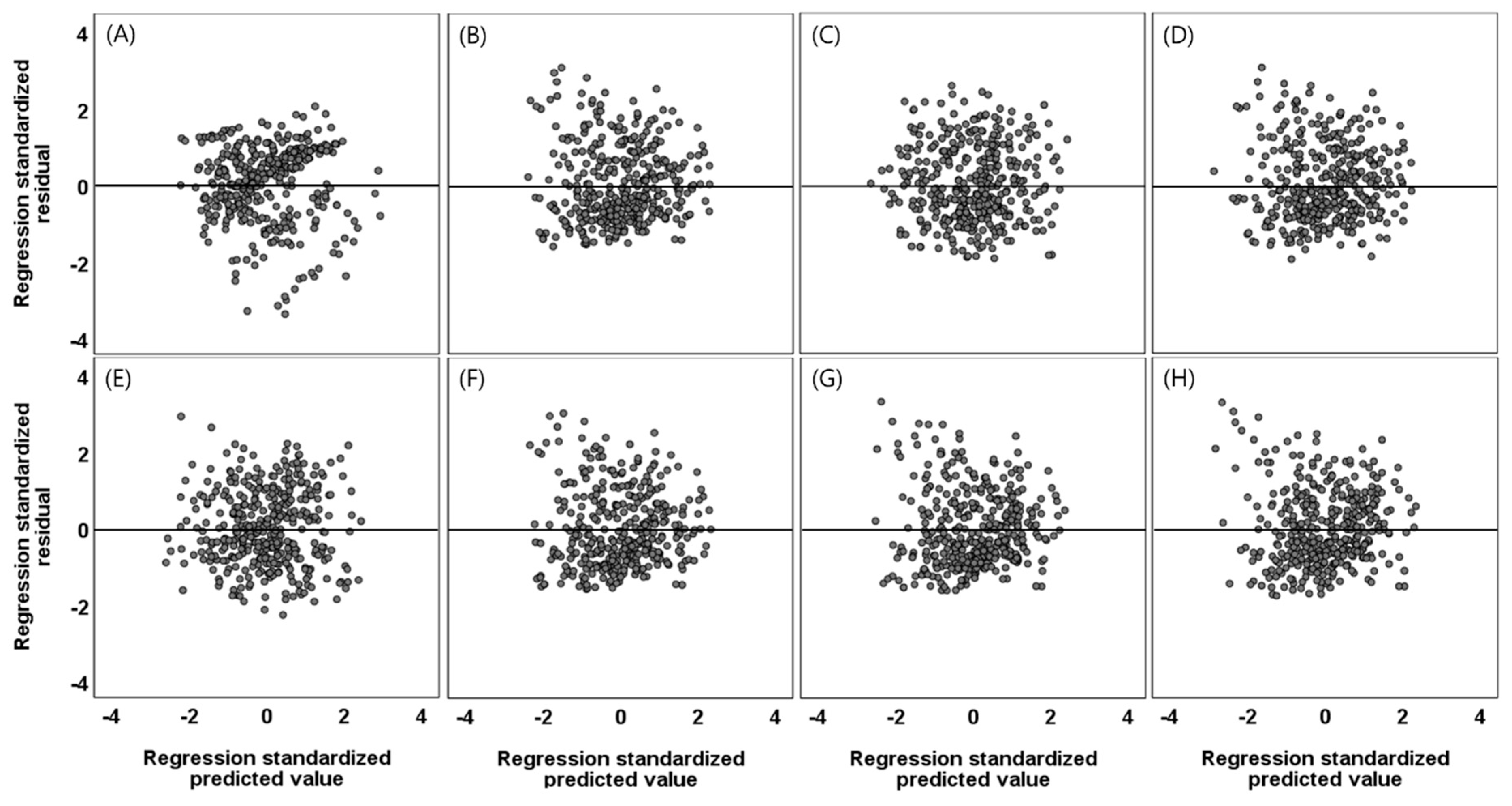
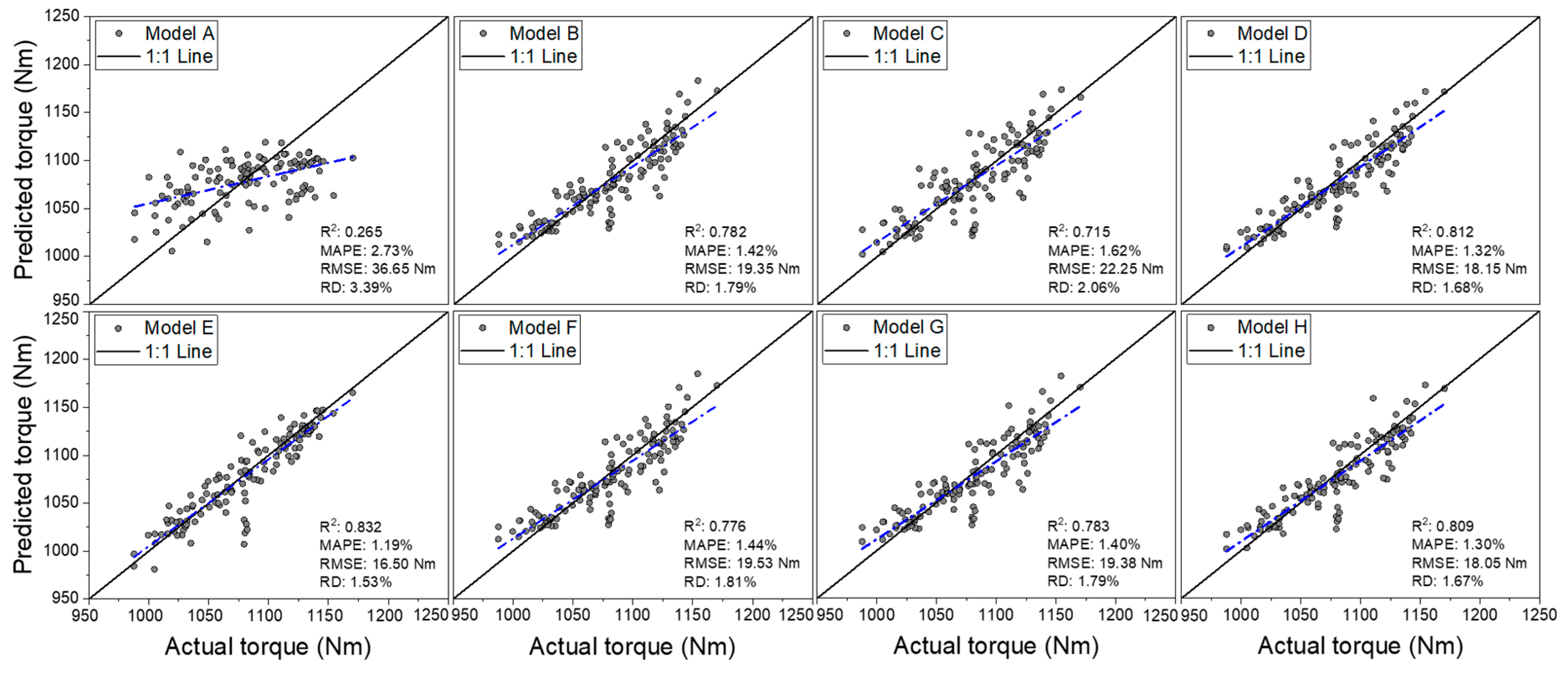
In this study, a prediction model was proposed for predicting tractor axle torque. A total of five variables were used to develop axle torque prediction models, and the Pearson correlation coefficients were highest in order of the tillage depth, slip ratio, travel speed, engine torque, and engine speed. The developed Model A using the engine parameter as a variable showed a low adjusted R² of 0.271, thus it is considered insufficient for use as a model for predicting axle torque. Nevertheless, in the case of Model D, which uses the engine parameter and tillage depth as variables, showed an adjusted R² of 0.877, and it is higher than that of Model B (R² adj: 0.866), which uses only the tillage depth as a single variable. Therefore, it is determined that the engine parameter can be used to improve prediction accuracy by combining it with other variables rather than using it in a prediction model as a single variable. Among the single sources, the tillage depth was regarded as the variable that could well explain the axle torque because it has high performance. In all the proposed models except Model A, the range of the adjusted R² were 0.813–0.925. These results were similar to the results of the prediction model for estimating the major parameters of the tractor such as the engine torque (R²: 0.835) [18], traction force (R²: 0.760–0.862) [23], and fuel consumption (R²: 0.892–0.916) [25]. The basic assumptions of regression analysis such as linearity, normality, independence, homoscedasticity, and multicollinearity were satisfied for all the proposed models except Model A. The D.W value in Model A is 1.34, and it may have difficulty guaranteeing the independence of the residuals. The verification results for the proposed model (MAPE: 1.19–3.61%) showed high prediction performance compared to the results of previous studies (Error: 1.27–3.61%) that predicted the theoretical axle torque according to the tillage depth [15]. Therefore, we believe that the proposed models can be applied to axle torque prediction. In conclusion, in this study, the developed prediction models can well explain the axle torque of the tractor using low-cost sensors or sensor data built into the tractor during tillage operation.

5. Conclusions

Tractor axle torque can be used by engineers as an index for making various decisions in transmission fatigue life analysis, optimal design, and life evaluation. However, the existing axle torque prediction method requires an expensive torque sensor. Therefore, this study developed a prediction model that can replace the existing expensive axle torque sensor. The purpose of this study was to develop a model that predicts tractor axle torque during tillage operation. In this study, a prediction model was proposed through regression analysis using the main variables affecting tractor axle torque.

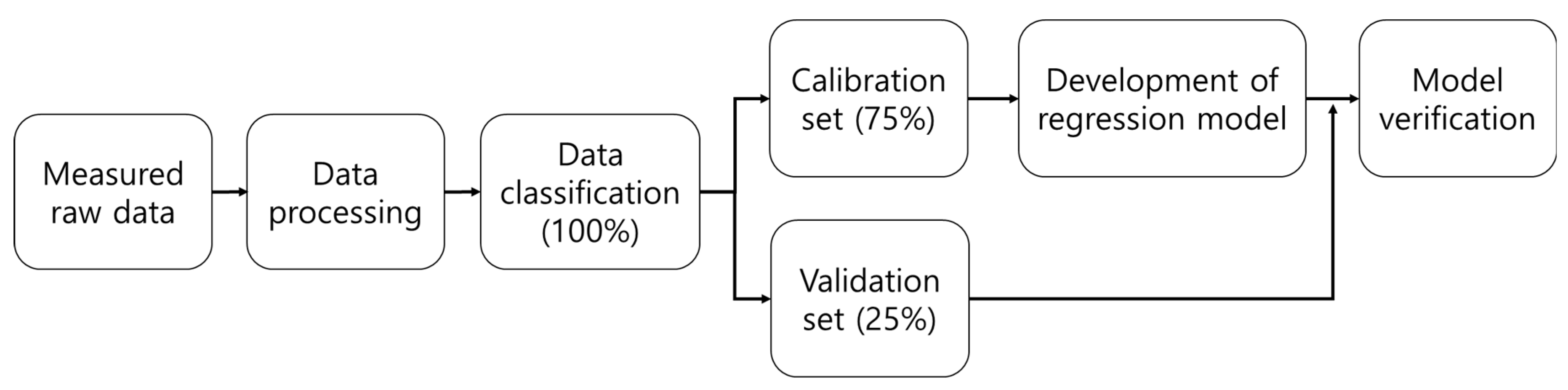
The engine parameters (engine torque and engine speed), tillage depth, travel speed, and slip ratio were selected as explanatory variables for the axle torque, which is the dependent variable. These were measured from the engine CAN communication, the built-in potentiometer installed on a three-point hitch, and the separately installed travel speed sensor. Field experiments were conducted using a tractor with a load measurement system to collect data for the explanatory variable and the dependent variable. The collected data were classified into a calibration set (75%) and a validation set (25%), which were used to develop and verify the regression analysis. A total of eight axle torque prediction regression models were proposed using each explanatory variable. The adjusted R² of the proposed regression model showed a range of 0.271 to 0.925. Among them, the prediction model E—with engine torque, engine speed, and travel speed as explanatory variables—showed an adjusted R² of 0.925. All the prediction models were tested for the basic assumptions of the regression analysis: linearity, normality, independence, homoscedasticity, and multicollinearity. All the prediction models proposed using the validation set were verified. As a result, all the prediction models showed an MAPE of less than 2.8%, and, in particular, Models E and H showed MAPEs of 1.19 and 1.30%, respectively, demonstrating a high accuracy. Therefore, it was found that the proposed prediction models are applicable to actual axle torque prediction.

This research is intended to propose a prediction model for each source, taking into account the data that the user can collect, because it is difficult for users to collect all the data. Since most previous studies focused on models for predicting engine torque, traction force, and fuel consumption, the main contribution of this study was to develop a low-cost sensor data-based axle torque prediction model. Despite these contributions, this study has limitation that the proposed model was developed and validated using data measured under limited working environment conditions (attached implement, gear stage, soil environment, and so on). The prediction model must be supplemented using data according to various conditions, because the tractor axle torque depends on various working conditions, such as the soil, gear stage, attached implement, ballast, etc. Therefore, in a future study, field data according to the various working conditions will be measured through experiments, and the prediction model will be expanded.

References

1. Baek, S.Y.; Kim, W.S.; Kim, Y.S.; Kim, Y.J.; Park, C.G.; An, S.C.; Moon, H.C.; Kim, B.S. Development of a simulation model for an 80 kW-class electric all-wheel-drive (AWD) tractor using agricultural workload. J. Drive Control 2020, 17, 27–36. [Google Scholar]
2. Kim, W.S.; Kim, Y.J.; Park, S.U.; Hong, S.J.; Kim, Y.S. Evaluation of PTO severeness for 78 kW-class tractor according to disk plow tillage and rotary tillage. J. Drive Control 2019, 16, 23–31. [Google Scholar]
3. Kim, W.S.; Kim, Y.S.; Kim, T.J.; Park, S.U.; Choi, Y.; Choi, I.S.; Kim, Y.K.; Kim, Y.J. Analysis of power requirement of 78 kW class agricultural tractor according to the major field operation. Trans. Korean Soc. Mech. Eng. A 2019, 43, 911–922. [Google Scholar] [CrossRef]
4. Kim, W.S.; Baek, S.Y.; Kim, T.J.; Kim, Y.S.; Park, S.U.; Choi, C.H.; Hong, S.J.; Kim, Y.J. Work load analysis for determination of the reduction gear ratio for a 78 kW all wheel drive electric tractor design. Korean J. Agric. Sci. 2019, 46, 613–627. [Google Scholar]
5. Park, S.J.; Kim, Y.J.; Lee, D.H. Analysis of load and fuel efficiency of agricultural tractor by gear selection during plow tillage. J. Food Agric. Environ. 2013, 11, 631–635. [Google Scholar]
6. Kim, Y.-S.; Kim, W.-S.; Baek, S.-Y.; Baek, S.-M.; Kim, Y.-J.; Lee, S.-D.; Kim, Y.-J. Analysis of Tillage Depth and Gear Selection for Mechanical Load and Fuel E ffi ciency of an Agricultural Tractor Using an Agricultural Field Measuring System. Sensors 2020, 20, 2450. [Google Scholar] [CrossRef] [PubMed]
7. Kim, W.-S.; Kim, Y.-J.; Kim, Y.-S.; Baek, S.-Y.; Baek, S.-M.; Lee, D.-H.; Nam, K.-C.; Kim, T.-B.; Lee, H.-J. Development of Control System for Automated Manual Transmission of 45-kW Agricultural Tractor. Appl. Sci. 2020, 10, 2930. [Google Scholar] [CrossRef]
8. Kim, Y.S.; Kim, T.J.; Kim, Y.J.; Lee, S.D.; Park, S.U.; Kim, W.S. Development of a real-time tillage depth measurement system for agricultural tractors : Application to the effect analysis of tillage depth on draft force during plow tillage. Sensors 2020, 20, 912. [Google Scholar] [CrossRef] [Green Version]
9. Han, K.H.; Kim, K.U.; Wu, Y.G. Severeness of transmission loads of agricultural tractor for rotary operations in poorly drained paddy field. J. Biosyst. Eng. 1999, 24, 293–300. [Google Scholar]
10. ASAE. Agricultural Machinery Management Data (D497.4). ASAE Standards 1999; ASAE: St. Joseph, MI, USA, 1999. [Google Scholar]
11. Upadhyay, G.; Raheman, H. Performance of combined offset disc harrow (front active and rear passive set configuration) in soil bin. J. Terramechanics 2018, 78, 27–37. [Google Scholar] [CrossRef]
12. Bashford, L.L.; Von Bargen, K.; Esch, J.H. Torque in agricultural tractor axles. SAE Trans. 1987, 96, 610–615. [Google Scholar]
13. Ashok Kumar, A.; Tewari, V.K.; Nare, B.; Chetan, C.R.; Srivastava, P.; Prakash Kumar, S. Embedded digital drive wheel torque indicator for agricultural 2WD tractors. Comput. Electron. Agric. 2017, 139, 91–102. [Google Scholar] [CrossRef]
14. Zoz, F.M.; Grisso, R.D. Traction and Tractor Performance; ASAE Disting. Lect. no. 27; ASAE: St. Joseph, MI, USA, 2003. [Google Scholar]
15. Kumar, A.A.; Tewari, V.K.; Nare, B. Embedded digital draft force and wheel slip indicator for tillage research. Comput. Electron. Agric. 2016, 127, 38–49. [Google Scholar] [CrossRef]
16. Brixius, W.W. Traction Prediction Equations for Bias Ply Tires. ASAE Paper 87-1622; ASAE: St. Joseph, MI, USA, 1987. [Google Scholar]
17. Rahimi-Ajdadi, F.; Abbaspour-Gilandeh, Y. Artificial Neural Network and stepwise multiple range regression methods for prediction of tractor fuel consumption. Meas. J. Int. Meas. Confed. 2011, 44, 2104–2111. [Google Scholar] [CrossRef]
18. Bietresato, M.; Calcante, A.; Mazzetto, F. A neural network approach for indirectly estimating farm tractors engine performances. Fuel 2015, 143, 144–154. [Google Scholar] [CrossRef]
19. Rajabi-Vandechali, M.; Abbaspour-Fard, M.H.; Rohani, A. Development of a prediction model for estimating tractor engine torque based on soft computing and low cost sensors. Measurement 2018, 121, 83–95. [Google Scholar] [CrossRef]
20. Elwaleed, A.K.; Yahya, A.; Zohadie, M.; Ahmad, D.; Kheiralla, A.F. Net traction ratio prediction for high-lug agricultural tyre. J. Terramechanics 2006, 43, 119–139. [Google Scholar] [CrossRef]
21. Roul, A.K.; Raheman, H.; Pansare, M.S.; Machavaram, R. Predicting the draught requirement of tillage implements in sandy clay loam soil using an artificial neural network. Biosyst. Eng. 2009, 104, 476–485. [Google Scholar] [CrossRef]
22. Hajiahmad, A.; Goli, H.; Jafari, A.; Keyhani, A.; Abdolmaleki, H. Side slip angle prediction model of an off-road tire on different terrains. J. Terramechanics 2014, 56, 25–35. [Google Scholar] [CrossRef]
23. Islam, M.N.; Iqbal, M.Z.; Kabir, M.S.N.; Jung, K.Y.; Mun, D.H.; Chung, S.O. Performance Evaluation of Trenchless Subsurface Drainage Piping Machine. J. Biosyst. Eng. 2019, 44, 218–225. [Google Scholar] [CrossRef]
24. Okyere, F.G.; Qasim, W.; Basak, J.K.; Khan, F.; Lee, Y.J.; Park, J.; Arulmozhi, E.; Yoon, Y.C.; Kang, D.S.; Kim, H.T. Analysis of draft force requirement of a compact disc harrow and model development for future predictions. J. Biosyst. Eng. 2019, 44, 47–56. [Google Scholar] [CrossRef]
25. Kheiralla, A.F.; Yahya, A.; Zohadie, M.; Ishak, W. Modelling of power and energy requirements for tillage implements operating in Serdang sandy clay loam, Malaysia. Soil Tillage Res. 2004, 78, 21–34. [Google Scholar] [CrossRef]
26. Lee, J.W.; Kim, J.S.; Kim, K.U. Computer simulations to maximise fuel efficiency and work performance of agricultural tractors in rotovating and ploughing operations. Biosyst. Eng. 2016, 142, 1–11. [Google Scholar] [CrossRef]
27. Upadhyay, G.; Raheman, H. Specific draft estimation model for offset disc harrows. Soil Tillage Res. 2019, 191, 75–84. [Google Scholar] [CrossRef]
28. Pitla, S.K.; Luck, J.D.; Werner, J.; Lin, N.; Shearer, S.A. In-field fuel use and load states of agricultural field machinery. Comput. Electron. Agric. 2016, 121, 290–300. [Google Scholar] [CrossRef] [Green Version]
29. Boon, N.E.; Yahya, A.; Kheiralla, A.F.; Wee, B.S.; Gew, S.K. A tractor-mounted, automated soil penetrometer-shearometer unit for mapping soil mechanical properties. Biosyst. Eng. 2005, 90, 381–396. [Google Scholar] [CrossRef]
30. Molari, G.; Bellentani, L.; Guarnieri, A.; Walker, M.; Sedoni, E. Performance of an agricultural tractor fitted with rubber tracks. Biosyst. Eng. 2012, 111, 57–63. [Google Scholar] [CrossRef]
31. Esch, J.H.; Bashford, L.L.; Von Bargen, K.; Ekstrom, R.E. Tractive performance comparisons between a rubber belt track and a four-wheel-drive tractor. Trans. ASAE 1990, 33, 1109–1115. [Google Scholar] [CrossRef]
32. Yahya, A.; Zohadie, M.; Kheiralla, A.F.; Giew, S.K.; Boon, N.E. Mapping system for tractor-implement performance. Comput. Electron. Agric. 2009, 69, 2–11. [Google Scholar] [CrossRef]
33. Kim, T.J.; Kim, W.S.; Kim, Y.S.; Chung, S.O.; Park, S.U.; Hong, S.J.; Choi, C.H.; Kim, Y.J. Strength analysis of mechanical transmission using equivalent torque of plow tillage of an 82 kW-class tractor. Korean J. Agric. Sci. 2019, 46, 723–735. [Google Scholar]
34. Park, S.U. Fatigue Life Evaluation of Spiral Bevel Gear of Transmission Using Agricultural Workload of Tractor; Chungnam National University: Daejeon, Korean, 2019. [Google Scholar]
35. ASABE Standard. Soil Cone Penetrometer (S313.3); ASABE: St. Joseph, MI, USA, 2018. [Google Scholar]
36. ASABE Standard. Procedures for Using and Reporting Data Obtained with the Soil Cone Penetrometer (EP542.1); ASABE: St. Joseph, MI, USA, 2019. [Google Scholar]
37. Shafaei, S.M.; Loghavi, M.; Kamgar, S. Reliable execution of a robust soft computing workplace found on multiple neuro-fuzzy inference systems coupled with multiple nonlinear equations for exhaustive perception of tractor-implement performance in plowing process. Artif. Intell. Agric. 2019, 2, 38–84. [Google Scholar] [CrossRef]
38. Rashidi, M.; Najjarzadeh, I.; Jaberinasab, B.; Emadi, S.M.; Fayyazi, M. Effect of soil moisture content, tillage depth and operation speed on draft force of moldboard plow. Middle East J. Sci. Res. 2013, 16, 245–249. [Google Scholar]
39. Ashok Kumar, A.; Tewari, V.K.; Gupta, C.; Pareek, C.M. A device to measure wheel slip to improve the fuel efficiency of off road vehicles. J. Terramechanics 2017, 70, 1–11. [Google Scholar] [CrossRef]
40. Kim, Y.J.; Chung, S.O.; Choi, C.H. Effects of gear selection of an agricultural tractor on transmission and PTO load during rotary tillage. Soil Tillage Res. 2013, 134, 90–96. [Google Scholar] [CrossRef]
41. Liao, J.; Hewitt, A.J.; Wang, P.; Luo, X.; Zang, Y.; Zhou, Z.; Lan, Y.; O’donnell, C. Development of droplet characteristics prediction models for air induction nozzles based on wind tunnel tests. Int. J. Agric. Biol. Eng. 2019, 12, 1–6. [Google Scholar] [CrossRef]
42. Slekovec, C.; Leroy, J.; Vernaz-Hegi, N.; Faller, J.P.; Sekri, D.; Hoen, B.; Talon, D.; Bertrand, X. Impact of a region wide antimicrobial stewardship guideline on urinary tract infection prescription patterns. Int. J. Clin. Pharm. 2012, 34, 325–329. [Google Scholar] [CrossRef] [PubMed]
43. Kim, B.; Yum, S.; Kim, Y.-Y.; Yun, N.; Shin, S.-Y.; You, S. An Analysis of Factors Relating to Agricultural Machinery Farm-Work Accidents Using Logistic Regression. J. Biosyst. Eng. 2014, 39, 151–157. [Google Scholar] [CrossRef] [Green Version]
44. O’Brien, R.M. A caution regarding rules of thumb for variance inflation factors. Qual. Quant. 2007, 41, 673–690. [Google Scholar] [CrossRef]
45. Kroll, C.N.; Song, P. Impact of multicollinearity on small sample hydrologic regression models. Water Resour. Res. 2013, 49, 3756–3769. [Google Scholar] [CrossRef]
46. Basak, J.K.; Qasim, W.; Okyere, F.G.; Khan, F.; Lee, Y.J.; Park, J.; Kim, H.T. Regression analysis to estimate morphology parameters of pepper plant in a controlled greenhouse system. J. Biosyst. Eng. 2019, 44, 57–68. [Google Scholar] [CrossRef]
47. Lobaskova, A. Need Some Fitspiration? Exploring Associations of Self-Construal and Gender Role Beliefs as well as a Mediating Role of Health Consciousness in “Thin and Toned” Social Media Ideal Internalization and Social Appearance Anxiety Outcomes Among Young Adult Fe. Master’s Thesis, University of Copenhagen, København Denmark, 2017. [Google Scholar]
Figure 1. Schematic diagram of a tractor power transmission system with prediction target axles.
Applsci 10 04195 g001
Figure 2. System installed on the tractor to collect field data for each major part: 1. Engine torque and engine speed, 2. Axle rotational speed, 3. Axle torque, 4. Travel speed, 5. Tillage depth, and 6. Data collection.
Applsci 10 04195 g002
Figure 3. Tractor with a moldboard plow used in the field experiment during tillage operation.
Applsci 10 04195 g003
Figure 4. Procedure for the development and verification of the prediction model using regression analysis.
Applsci 10 04195 g004
Figure 5. The distribution of the regression standardized residuals for each prediction Model (AH): Model A = axle torque as a linear function of engine torque and engine speed; Model B = axle torque as a linear function of tillage depth; Model C = axle torque as a linear function of slip ratio and travel speed; Model D = axle torque as a linear function of engine torque, engine speed and tillage depth; Model E = axle torque as a linear function of engine torque, engine speed and travel speed; Model F = axle torque as a linear function of tillage depth and travel speed; Model G = axle torque as a linear function of engine speed, tillage depth and travel speed; and Model H = axle torque as a linear function of engine torque, tillage depth and travel speed.
Applsci 10 04195 g005
Figure 6. P–P plots of the regression-normalized residuals of the expected cumulative probability versus actual cumulative probability for each regression Model (AH): Model A = axle torque as a linear function of engine torque and engine speed; Model B = axle torque as a linear function of tillage depth; Model C = axle torque as a linear function of slip ratio and travel speed; Model D = axle torque as a linear function of engine torque, engine speed and tillage depth; Model E = axle torque as a linear function of engine torque, engine speed and travel speed; Model F = axle torque as a linear function of tillage depth and travel speed; Model G = axle torque as a linear function of engine speed, tillage depth and travel speed; and Model H = axle torque as a linear function of engine torque, tillage depth and travel speed.
Applsci 10 04195 g006
Figure 7. Scatter plot of the standardized predicted values and standardized residuals for each regression Model (AH): Model A = axle torque as a linear function of engine torque and engine speed; Model B = axle torque as a linear function of tillage depth; Model C = axle torque as a linear function of slip ratio and travel speed; Model D = axle torque as a linear function of engine torque, engine speed and tillage depth; Model E = axle torque as a linear function of engine torque, engine speed and travel speed; Model F = axle torque as a linear function of tillage depth and travel speed; Model G = axle torque as a linear function of engine speed, tillage depth and travel speed; and Model H = axle torque as a linear function of engine torque, tillage depth and travel speed.
Applsci 10 04195 g007
Figure 8. Relationships between the predicted and measured axle torque for each regression Model (AH): Model A = axle torque as a linear function of engine torque and engine speed; Model B = axle torque as a linear function of tillage depth; Model C = axle torque as a linear function of slip ratio and travel speed; Model D = axle torque as a linear function of engine torque, engine speed and tillage depth; Model E = axle torque as a linear function of engine torque, engine speed and travel speed; Model F = axle torque as a linear function of tillage depth and travel speed; Model G = axle torque as a linear function of engine speed, tillage depth and travel speed; and Model H = axle torque as a linear function of engine torque, tillage depth and travel speed.
Applsci 10 04195 g008