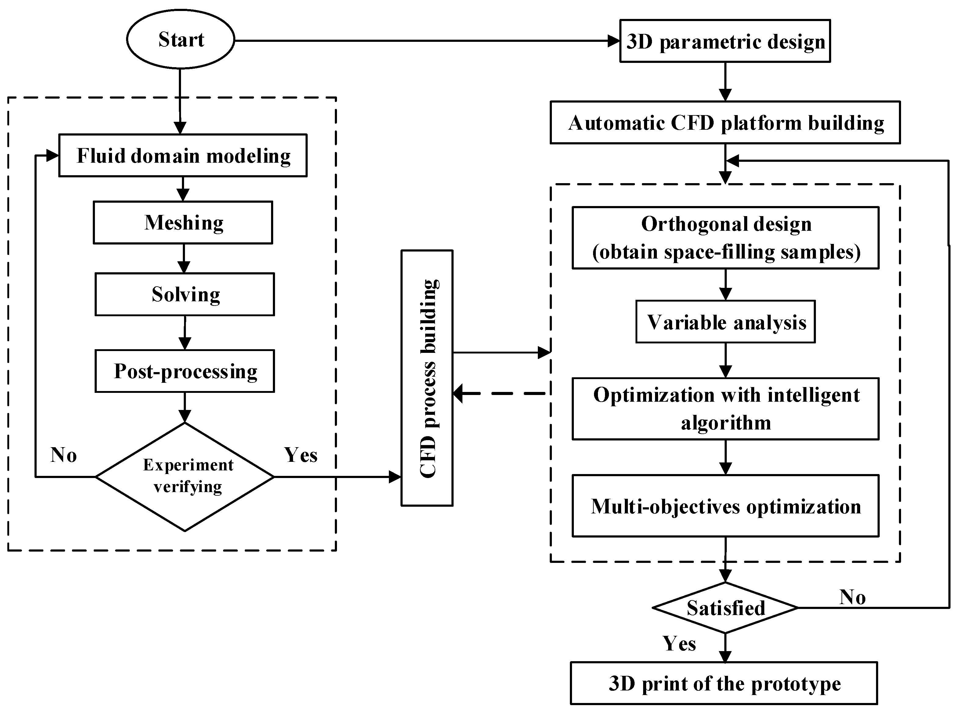
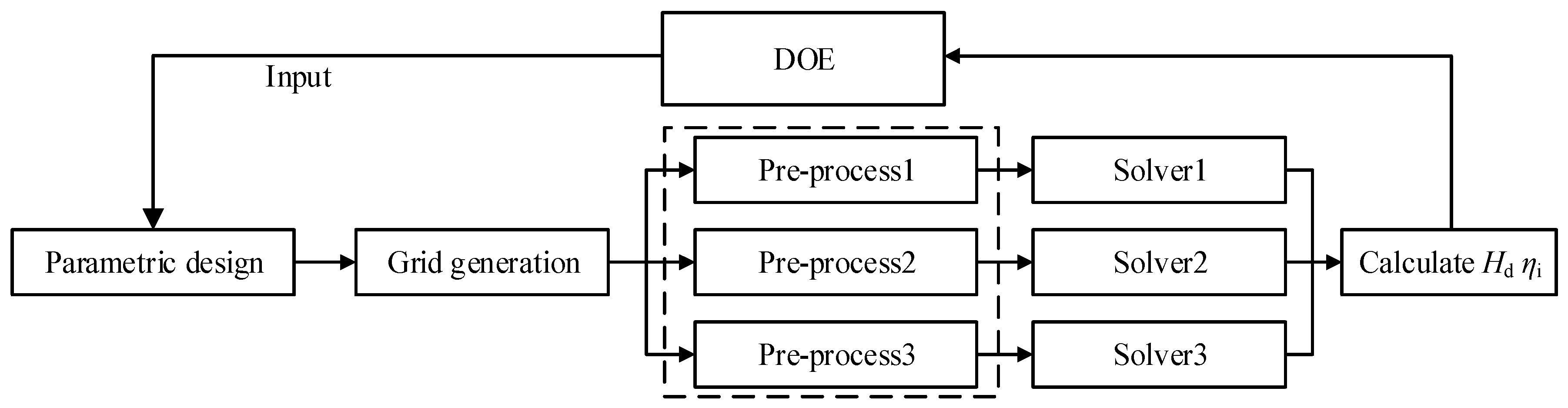
Figure 1.
The flowchart of optimization process. CFD, computational fluid dynamics.
Figure 1.
The flowchart of optimization process. CFD, computational fluid dynamics.
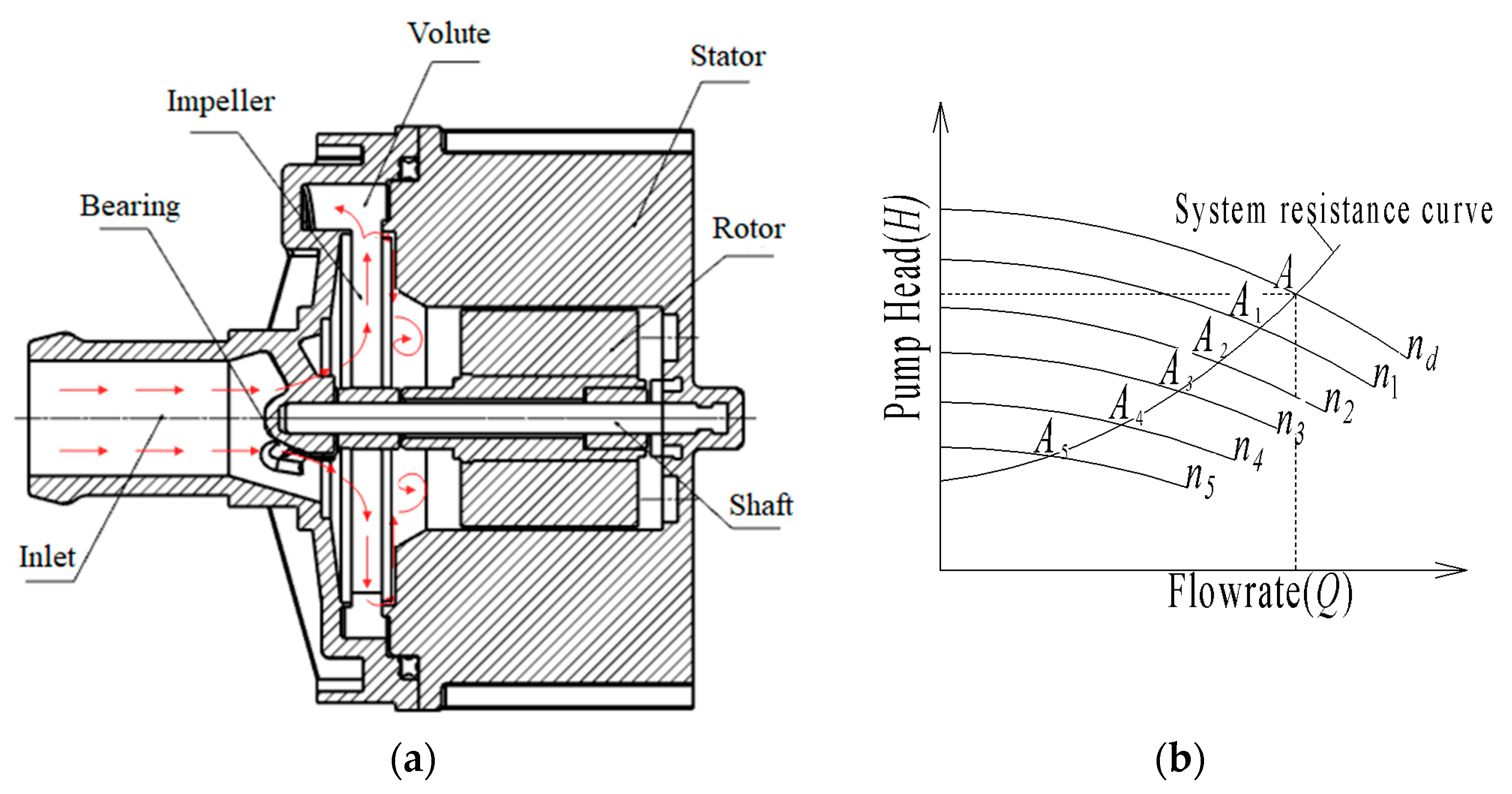
Figure 2.
Automobile electronic pump model: (a) Structure diagram; (b) Performance characteristic curves.
Figure 2.
Automobile electronic pump model: (a) Structure diagram; (b) Performance characteristic curves.
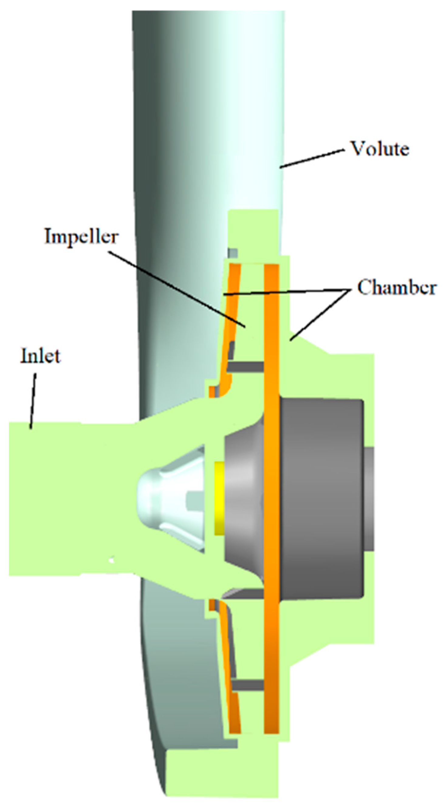
Figure 3.
Model of computational domains.
Figure 3.
Model of computational domains.
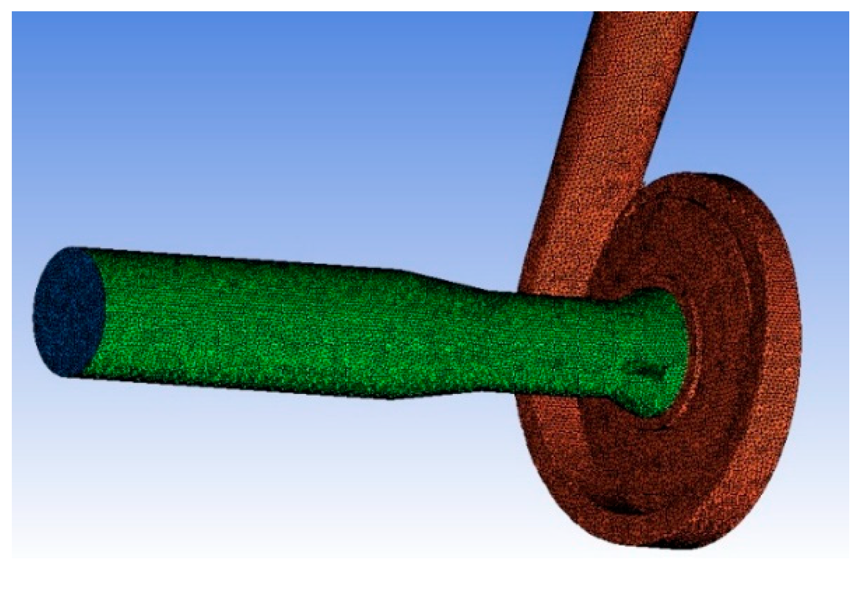
Figure 4.
Computational meshes.
Figure 4.
Computational meshes.
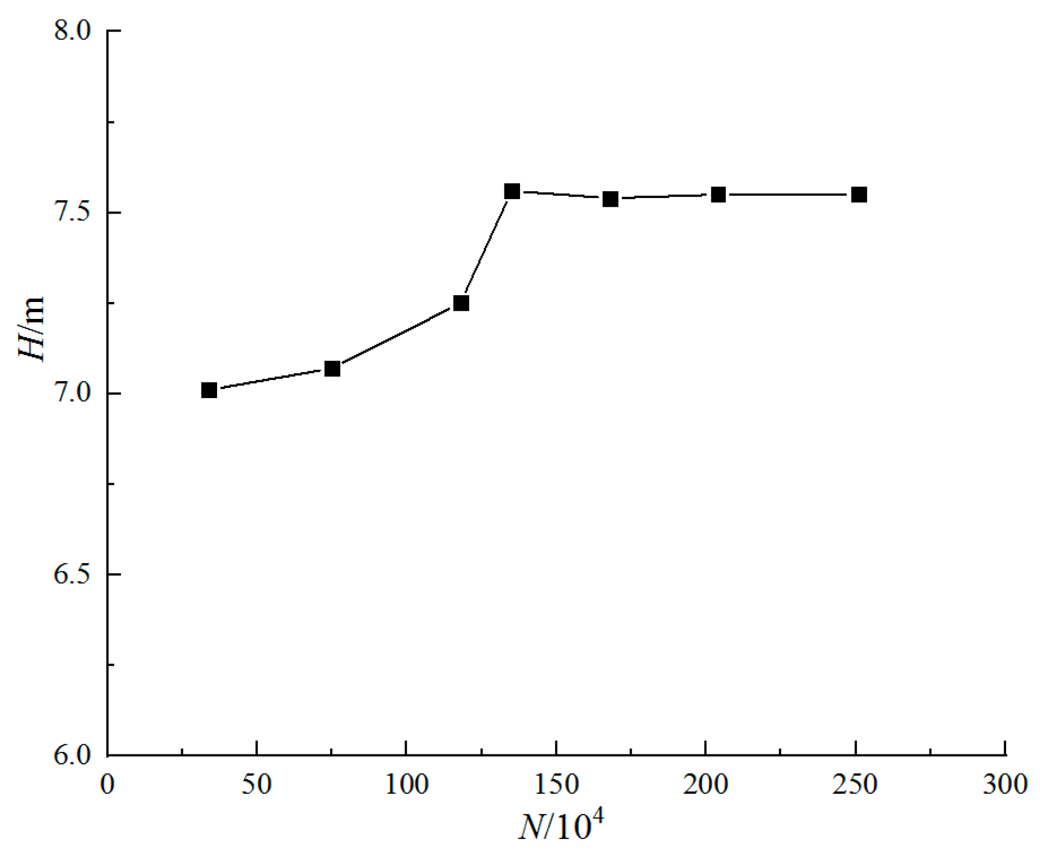
Figure 5.
Analysis of grid independence.
Figure 5.
Analysis of grid independence.
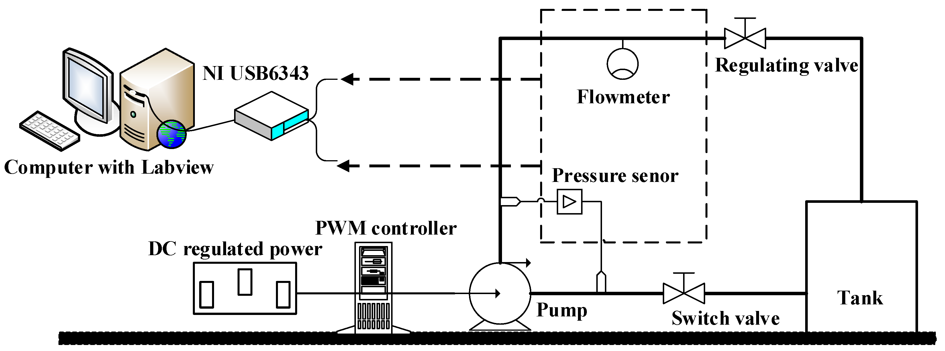
Figure 6.
The schematic diagram of test rig.
Figure 6.
The schematic diagram of test rig.
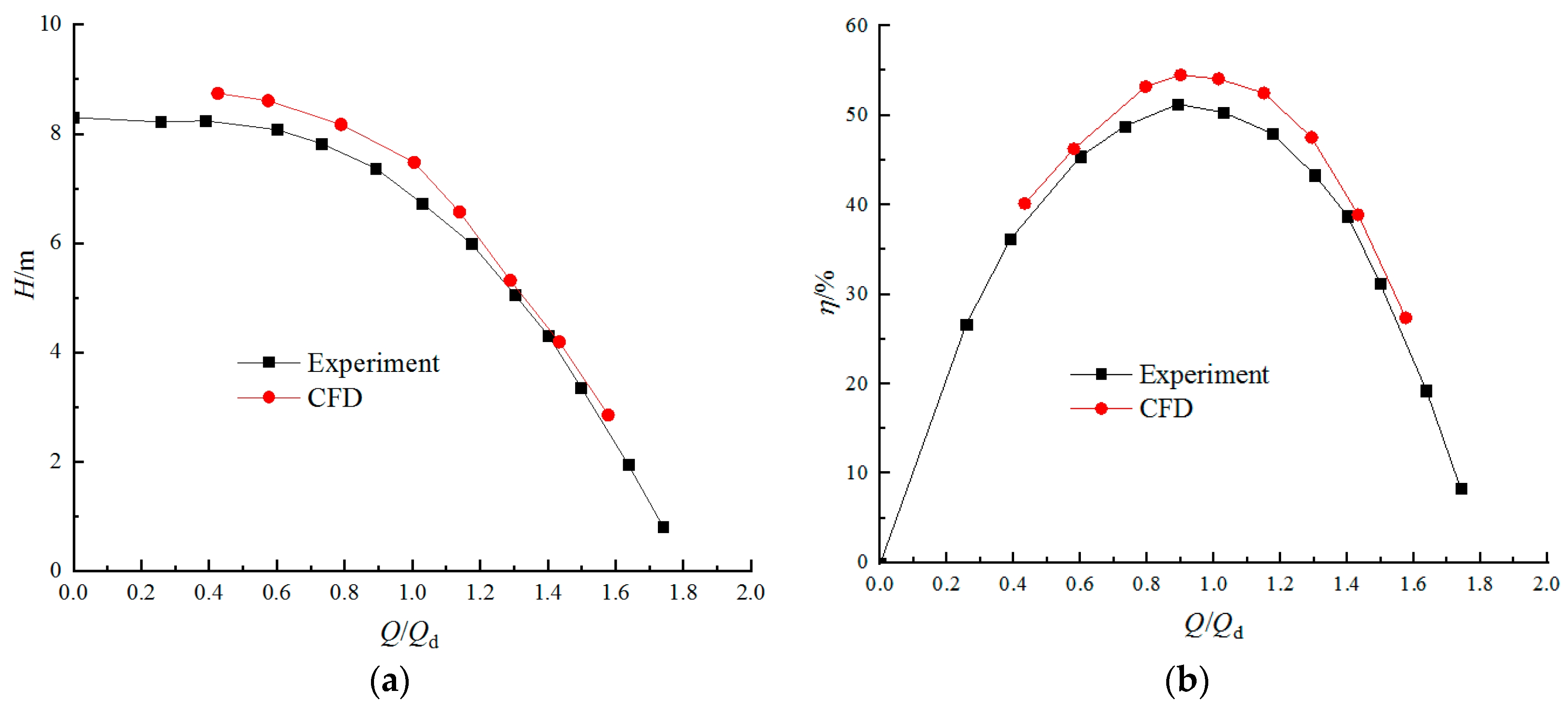
Figure 7.
Comparison of pump performance between numerical and experimental results: (a) Head; (b) Efficiency.
Figure 7.
Comparison of pump performance between numerical and experimental results: (a) Head; (b) Efficiency.
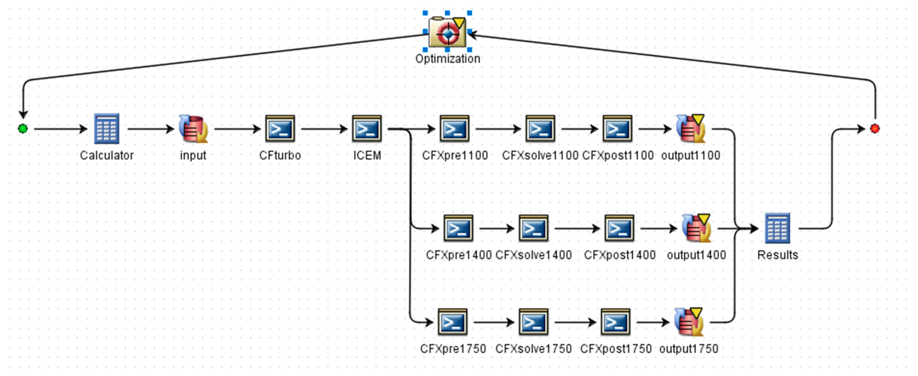
Figure 8.
Operation process of the automatic optimization platform.
Figure 8.
Operation process of the automatic optimization platform.
Figure 9.
Integrated optimization platform of automotive electronic water pump.
Figure 9.
Integrated optimization platform of automotive electronic water pump.
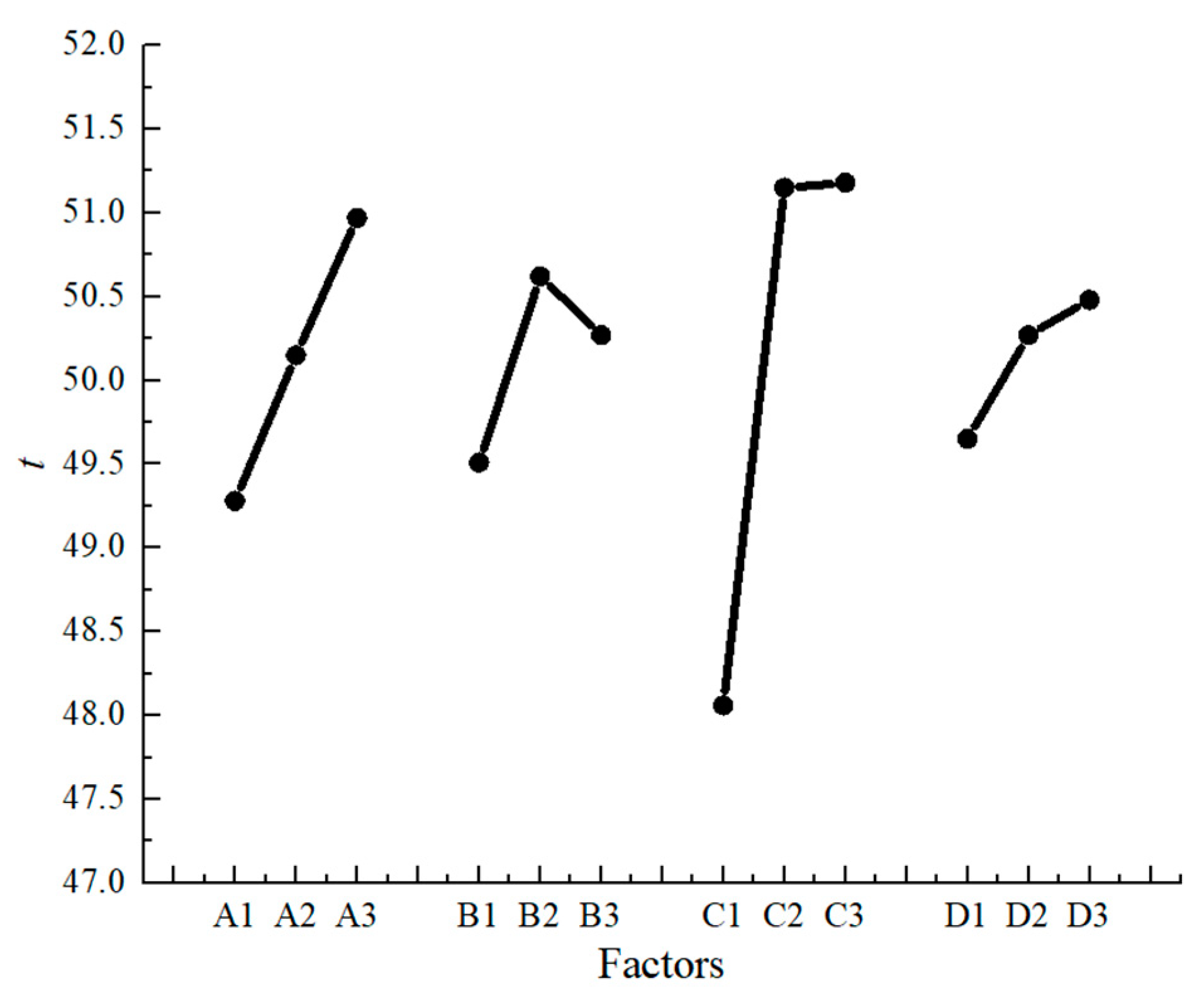
Figure 10.
Range analysis diagram.
Figure 10.
Range analysis diagram.
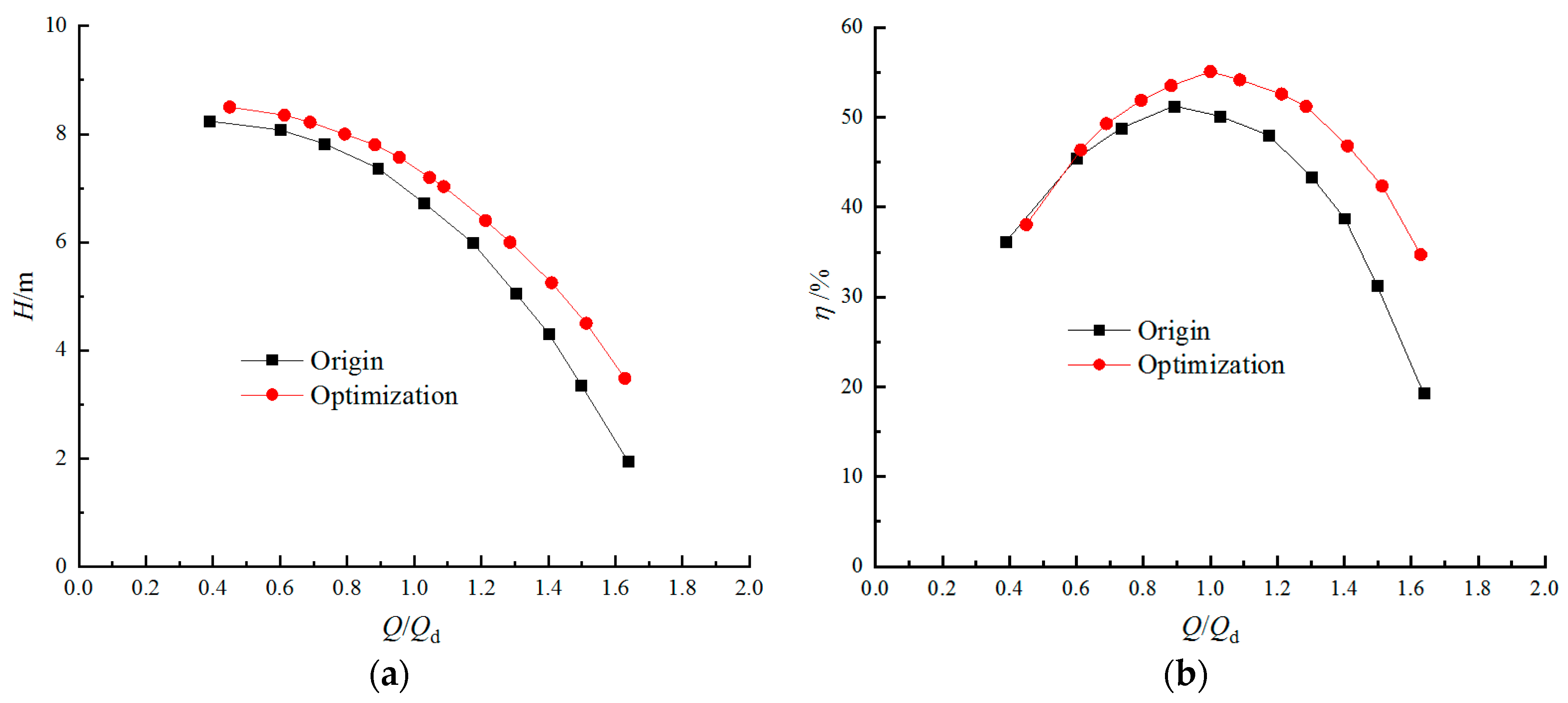
Figure 11.
Comparison of external characteristic curves between origin and optimization scheme: (a) Head; (b) Efficiency.
Figure 11.
Comparison of external characteristic curves between origin and optimization scheme: (a) Head; (b) Efficiency.
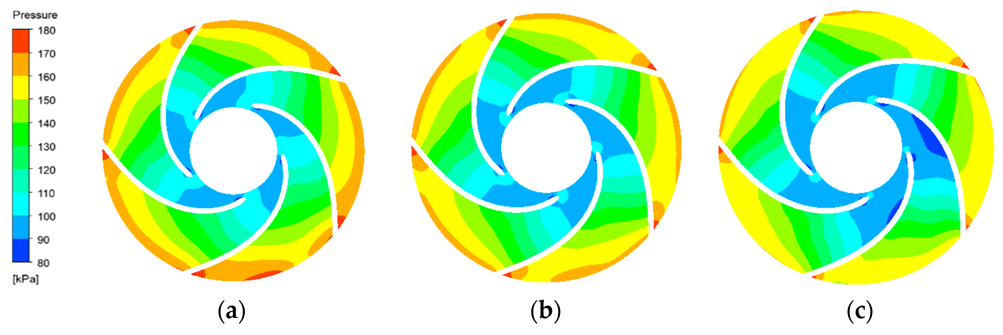
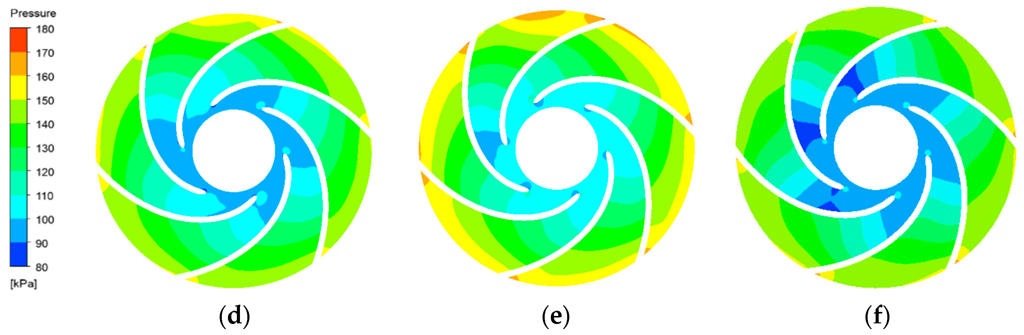
Figure 12.
Comparison of pressure distribution in impeller for the two schemes: (a) origin, 0.8Qd; (b) origin, 1.0Qd; (c) origin, 1.25Qd; (d) optimization, 0.8Qd; (e) optimization, 1.0Qd; (f) optimization, 1.25Qd.
Figure 12.
Comparison of pressure distribution in impeller for the two schemes: (a) origin, 0.8Qd; (b) origin, 1.0Qd; (c) origin, 1.25Qd; (d) optimization, 0.8Qd; (e) optimization, 1.0Qd; (f) optimization, 1.25Qd.
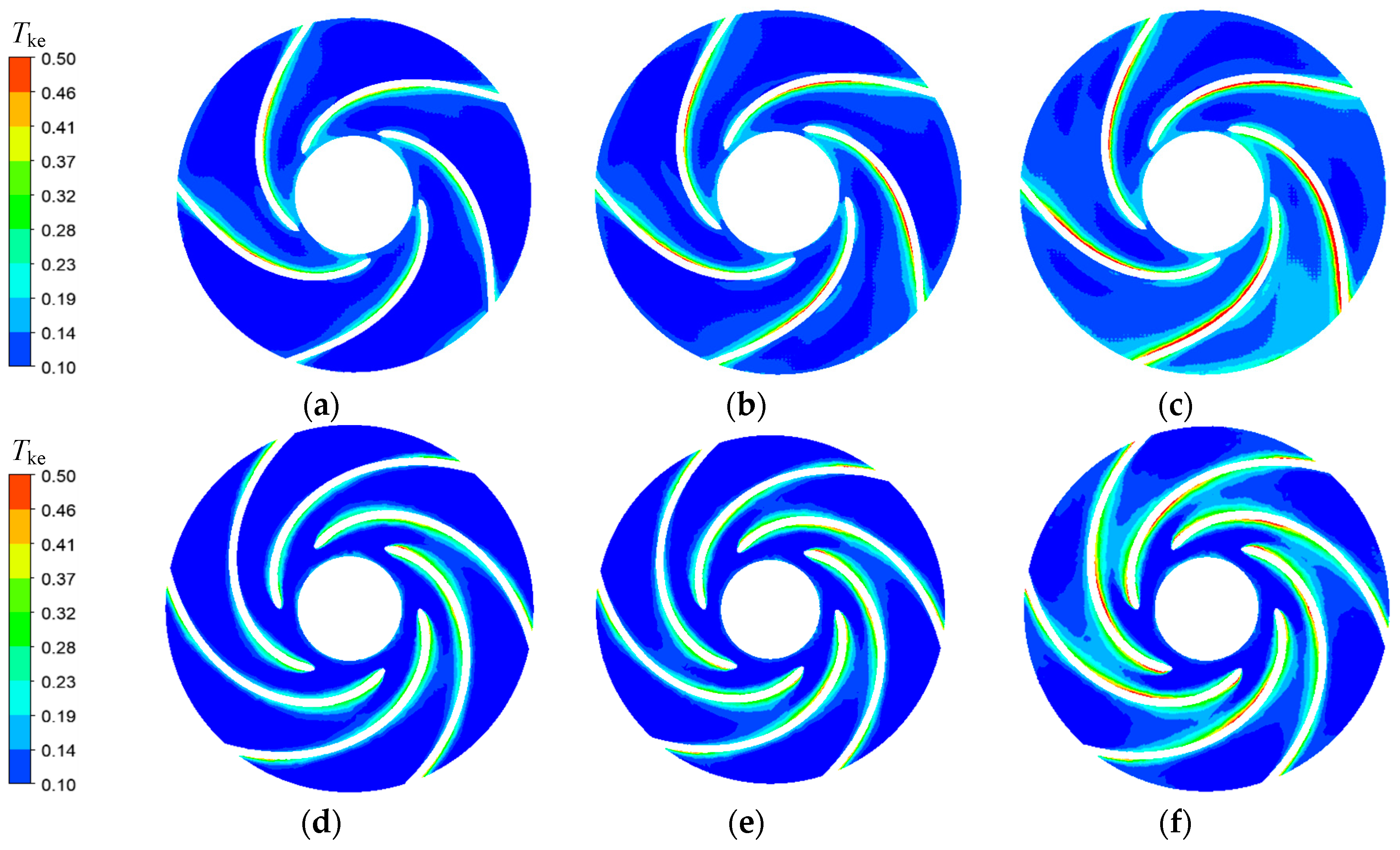
Figure 13.
Comparison of turbulence kinetic energy in impeller for the two schemes: (a) origin, 0.8Qd; (b) origin, 1.0Qd; (c) origin, 1.25Qd; (d) optimization, 0.8Qd; (e) optimization, 1.0Qd; (f) optimization, 1.25Qd.
Figure 13.
Comparison of turbulence kinetic energy in impeller for the two schemes: (a) origin, 0.8Qd; (b) origin, 1.0Qd; (c) origin, 1.25Qd; (d) optimization, 0.8Qd; (e) optimization, 1.0Qd; (f) optimization, 1.25Qd.
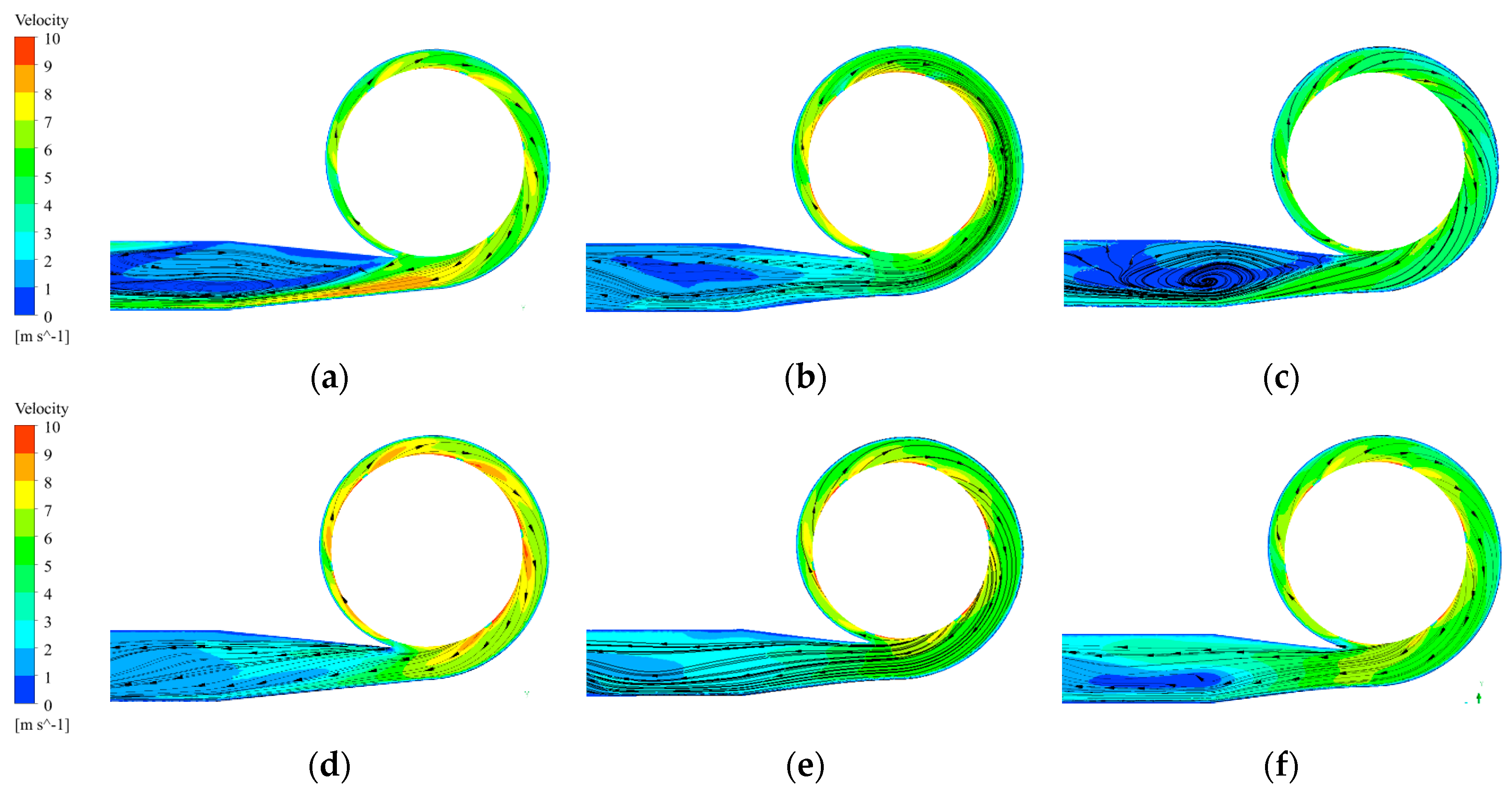
Figure 14.
Comparison of velocity streamline in volute for the two schemes: (a) origin, 0.8Qd; (b) origin, 1.0Qd; (c) origin, 1.25Qd; (d) optimization, 0.8Qd; (e) optimization, 1.0Qd; (f) optimization, 1.25Qd.
Figure 14.
Comparison of velocity streamline in volute for the two schemes: (a) origin, 0.8Qd; (b) origin, 1.0Qd; (c) origin, 1.25Qd; (d) optimization, 0.8Qd; (e) optimization, 1.0Qd; (f) optimization, 1.25Qd.
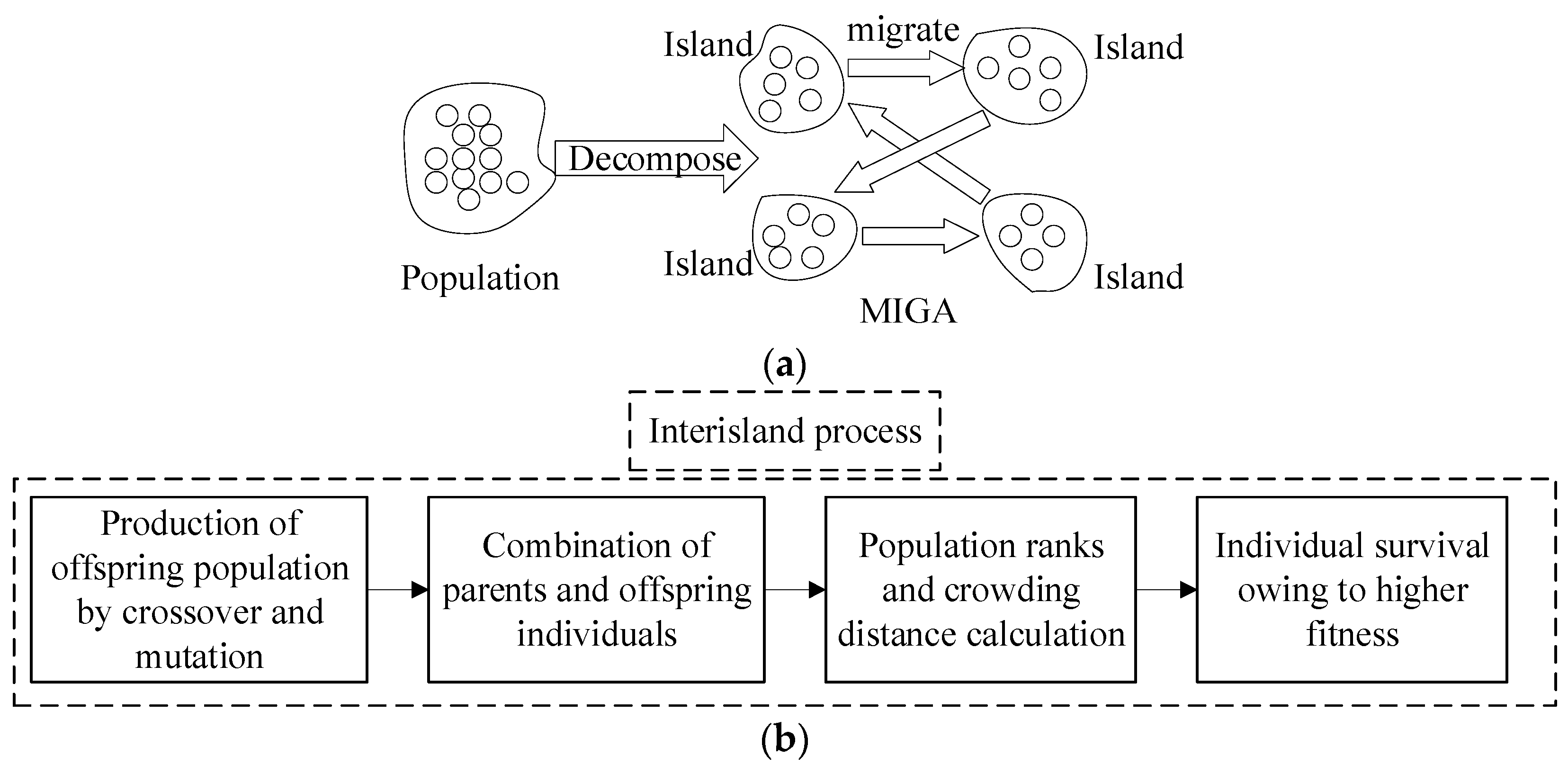
Figure 15.
The structure and process of the multi-island genetic algorithm (MIGA) optimization method: (a) Structure, (b) Process.
Figure 15.
The structure and process of the multi-island genetic algorithm (MIGA) optimization method: (a) Structure, (b) Process.
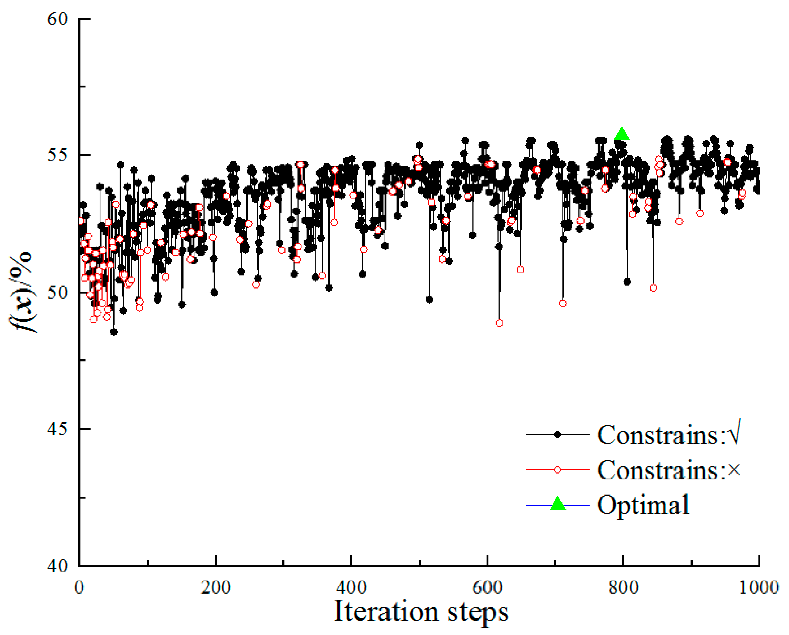
Figure 16.
The iteration process of optimization.
Figure 16.
The iteration process of optimization.
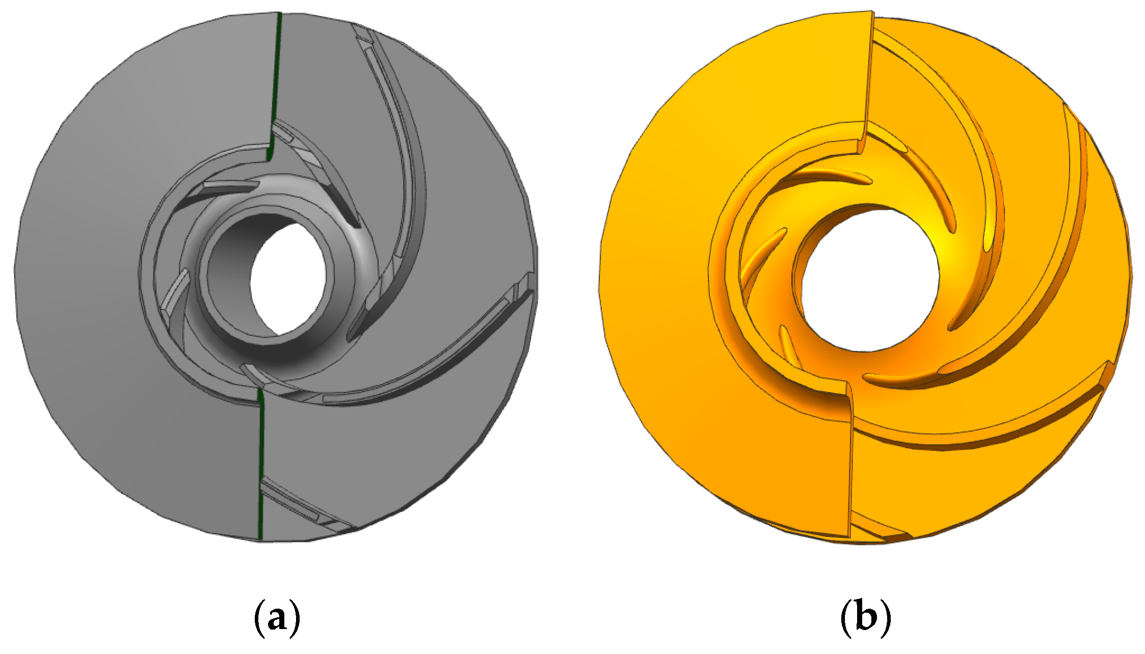
Figure 17.
Comparison of impeller model: (a) scheme 1; (b) scheme 3.
Figure 17.
Comparison of impeller model: (a) scheme 1; (b) scheme 3.
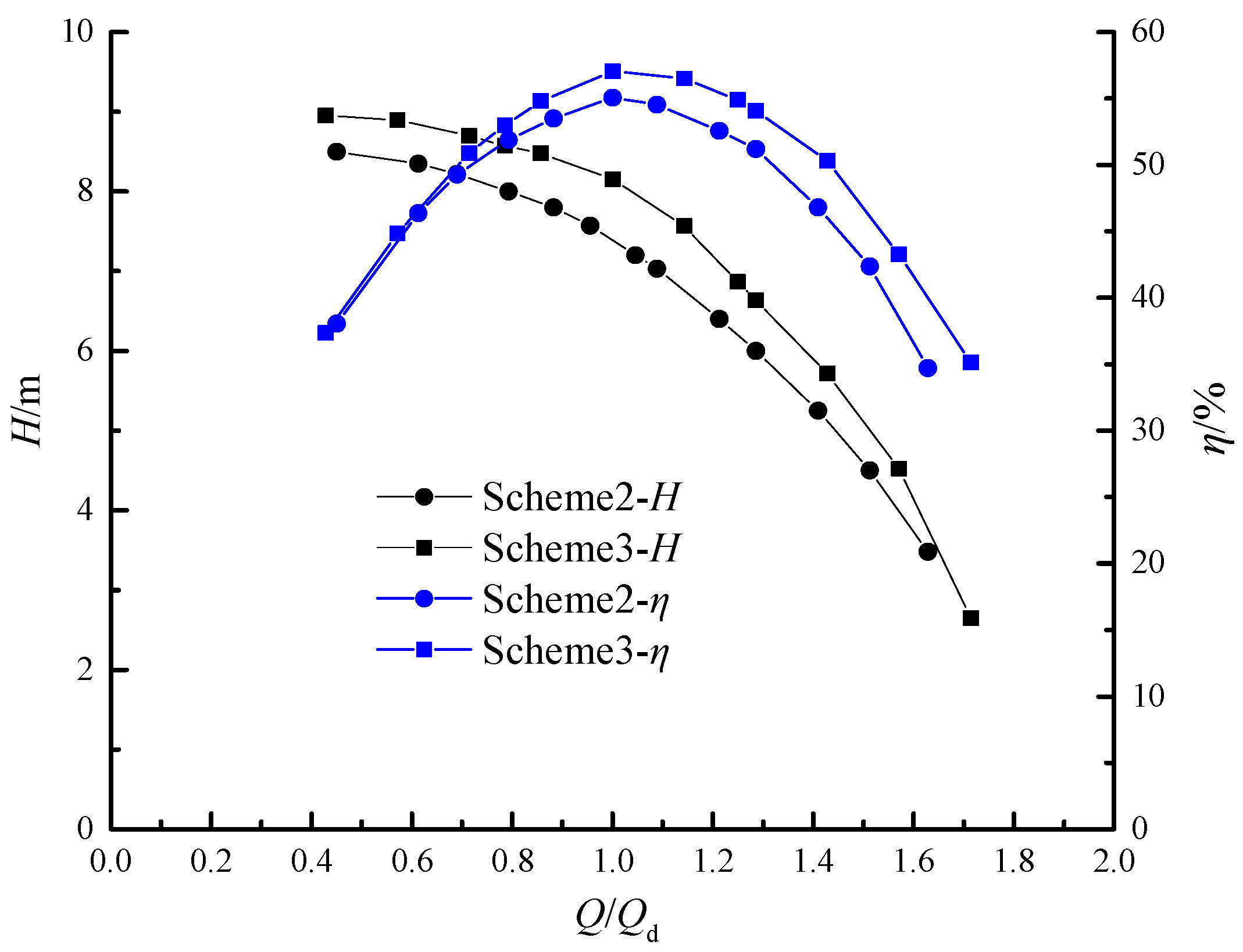
Figure 18.
Comparison of external characteristic curves.
Figure 18.
Comparison of external characteristic curves.
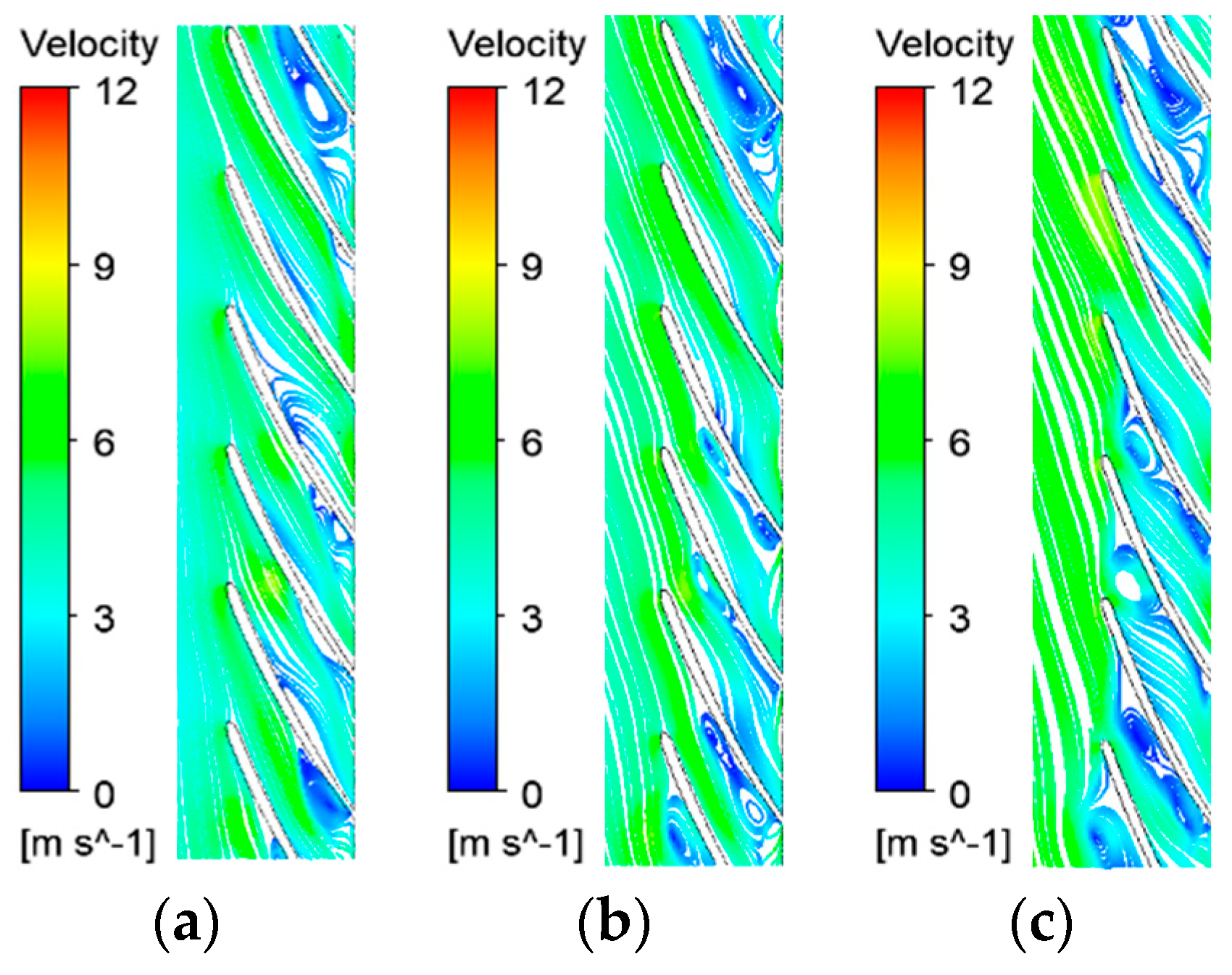
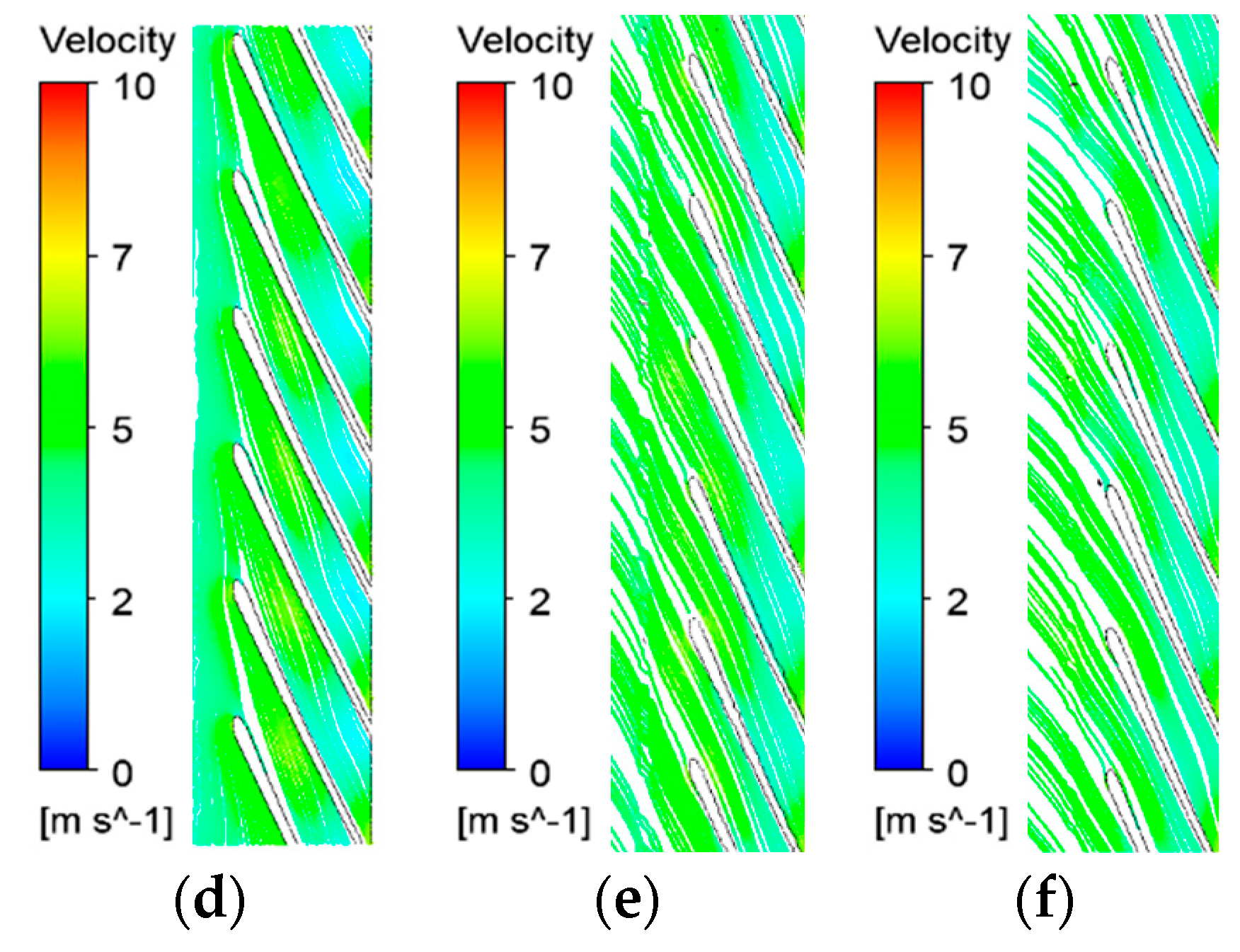
Figure 19.
Comparison of streamline at different spans under 1.0Qd: (a) Origin scheme 1, span = 10%; (b) Origin scheme 1, span = 50%; (c) Origin scheme 1, span = 90%; (d) Optimal scheme 3, span = 10%; (e) Optimal scheme 3, span = 50%; (f) Optimal scheme 3, span = 90%.
Figure 19.
Comparison of streamline at different spans under 1.0Qd: (a) Origin scheme 1, span = 10%; (b) Origin scheme 1, span = 50%; (c) Origin scheme 1, span = 90%; (d) Optimal scheme 3, span = 10%; (e) Optimal scheme 3, span = 50%; (f) Optimal scheme 3, span = 90%.
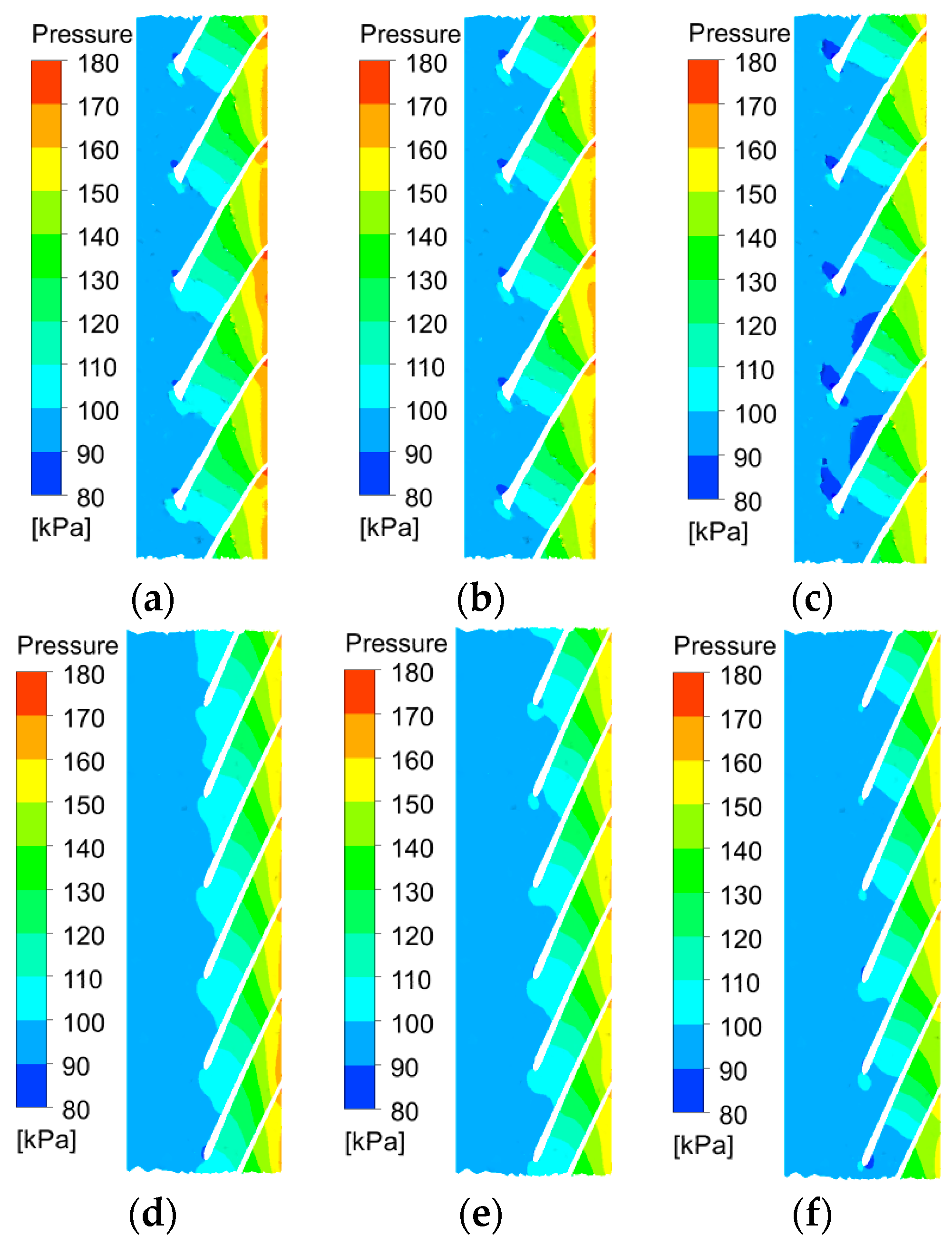
Figure 20.
Pressure comparison at span = 90% under different working conditions: (a) Origin, 0.8Qd; (b) Origin,1.0Qd; (c) Origin, 1.25Qd; (d) Optimal, 0.8Qd; (e) Optimal, 1.0Qd; (f) Optimal, 1.25Qd.
Figure 20.
Pressure comparison at span = 90% under different working conditions: (a) Origin, 0.8Qd; (b) Origin,1.0Qd; (c) Origin, 1.25Qd; (d) Optimal, 0.8Qd; (e) Optimal, 1.0Qd; (f) Optimal, 1.25Qd.
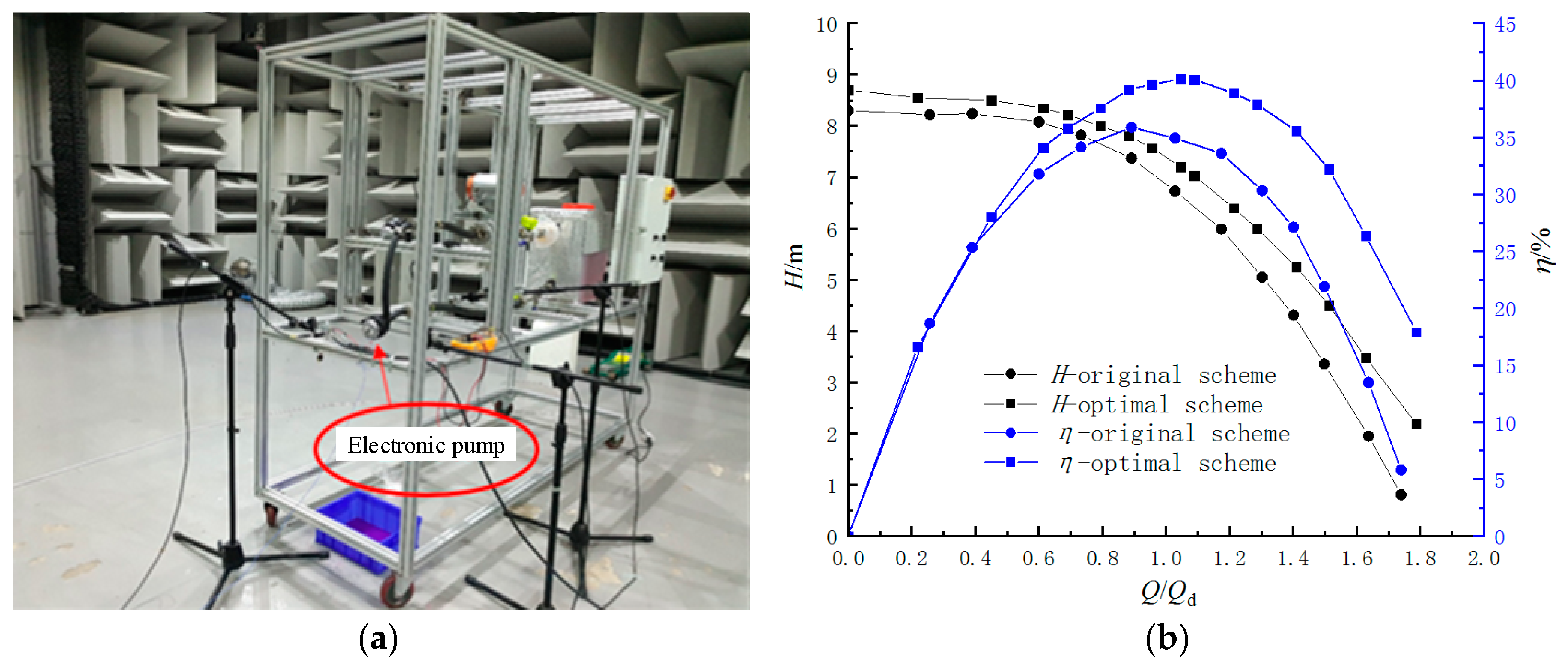
Figure 21.
Comparison of the origin and optimal scheme. (a) Test rig; (b) Comparison pump performance results.
Figure 21.
Comparison of the origin and optimal scheme. (a) Test rig; (b) Comparison pump performance results.
Table 1.
Main geometric parameters of the pump.
Table 1.
Main geometric parameters of the pump.
| Description | Parameter | Symbol | Unit | Value |
|---|
| Impeller | Inlet diameter | D1 | mm | 20 |
| Outlet diameter | D2 | mm | 47 |
| Outlet width | b2 | mm | 2.2 |
| Blade inlet angle | β1 | ° | 20 |
| Blade number | Z | - | 5 |
| Blade outlet angle | β2 | ° | 41 |
| Volute | Inlet diameter | D3 | mm | 50 |
| Inlet width | b3 | mm | 6 |
| Pipe diameter | D | mm | 17 |
Table 2.
Random consistency index (RI).
Table 2.
Random consistency index (RI).
| N | 1 | 2 | 3 | 4 | 5 | 6 | 7 | 8 | 9 | 10 | 11 |
| RI | 0 | 0 | 0.58 | 0.9 | 1.12 | 1.24 | 1.34 | 1.41 | 1.45 | 1.49 | 1.51 |
Table 3.
Levels of factors in orthogonal experiments.
Table 3.
Levels of factors in orthogonal experiments.
| Levels | Factors |
|---|
A
D2/mm | B
b2/mm | C
Z | D
β2/(°) |
|---|
| 1 | 44 | 3 | 4 | 30 |
| 2 | 45 | 3.2 | 5 | 33 |
| 3 | 46 | 3.5 | 6 | 35 |
Table 4.
Evaluation results and weight factors. CR, consistency ratio.
Table 4.
Evaluation results and weight factors. CR, consistency ratio.
| Objective | η1 | η2 | η3 | ωi |
|---|
| η1 | 1 | 2/3 | 10/11 | 0.2786 |
| η2 | 3/2 | 1 | 5/4 | 0.4059 |
| η3 | 11/10 | 4/5 | 1 | 0.3155 |
| CR | | 0.000725 | | |
Table 5.
Test schemes.
| Number | Levels | Corresponding Parameters | Results |
|---|
| A | B | C | D | D2 | b2 | Z | β2 | f(X) |
|---|
| 1 | A1 | B1 | C1 | D1 | 44 | 3 | 4 | 30 | 46.11 |
| 2 | A1 | B2 | C2 | D2 | 44 | 3.2 | 5 | 33 | 50.92 |
| 3 | A1 | B3 | C3 | D3 | 44 | 3.5 | 6 | 35 | 50.81 |
| 4 | A2 | B1 | C2 | D3 | 45 | 3 | 5 | 35 | 50.89 |
| 5 | A2 | B2 | C3 | D1 | 45 | 3.2 | 6 | 30 | 51.21 |
| 6 | A2 | B3 | C1 | D2 | 45 | 3.5 | 4 | 33 | 48.35 |
| 7 | A3 | B1 | C3 | D2 | 46 | 3 | 6 | 33 | 51.53 |
| 8 | A3 | B2 | C1 | D3 | 46 | 3.2 | 4 | 35 | 49.73 |
| 9 | A3 | B3 | C2 | D1 | 46 | 3.5 | 5 | 30 | 51.64 |
Table 6.
Range analysis.
| Target | |
|---|
| A | B | C | D |
|---|
| t1 | 49.28 | 49.51 | 48.06 | 49.65 |
| t2 | 50.15 | 50.62 | 51.15 | 50.27 |
| t3 | 50.97 | 50.27 | 51.18 | 50.48 |
| R | 1.69 | 1.11 | 3.12 | 0.83 |
Table 7.
Analysis of variance.
Table 7.
Analysis of variance.
| Source of Variance | |
|---|
| A | B | C | D |
|---|
| Sum of squared deviation SST | 4.269 | 1.929 | 19.263 | 1.098 |
| Degree of freedom fT | 2 | 2 | 2 | 2 |
| Mean square error SSE | 1.1 | 1.1 | 1.1 | 1.1 |
| Statistics value Fk | 3.888 | 1.757 | 17.544 | 1 |
| Significance | Insignificant | Insignificant | Significant | Insignificant |
Table 8.
Comparison of the performances under specified conditions.
Table 8.
Comparison of the performances under specified conditions.
| Operation Points | H/m | η/% | Weighted Average Efficiency % |
|---|
| Original | Optimal | Original | Optimal | Original | Optimal |
|---|
| 0.8Qd | 7.6 | 7.9 | 50.1 | 52.17 | 49.93 | 53.22 |
| 1.0Qd | 6.7 | 7.3 | 51.4 | 55.06 |
| 1.25Qd | 5.35 | 6.15 | 47.97 | 51.8 |
Table 9.
Ranges of optimization variables.
Table 9.
Ranges of optimization variables.
| Parameters | Ranges |
|---|
| D2(mm) | (45, 47) |
| b2(mm) | (2.5, 3.5) |
| β1(°) | (20, 30) |
| β2(°) | (30, 40) |
| t3 (°) | (0, 25) |
| ϕ (°) | (100, 120) |
| δ (mm) | (2, 6) |
Table 10.
Optimization parameters adopted in MIGA.
Table 10.
Optimization parameters adopted in MIGA.
| Parameters | Numerical Value |
|---|
| Generations | 10 |
| Subpopulation Size | 10 |
| Number of Islands | 10 |
| Crossover rate | 0.9 |
| Migration rate | 0.01 |
| Interval of Migration | 5 |
| Mutation Rate | 0.01 |
Table 11.
Comparison of geometric parameters between scheme 2 and scheme 3.
Table 11.
Comparison of geometric parameters between scheme 2 and scheme 3.
| Parameters | Symbols | Unit | Scheme 2 | Scheme 3 |
|---|
| Outlet diameter | D2 | mm | 46 | 45 |
| Outlet width | b2 | mm | 3.2 | 3.4 |
| Blade number | Z | - | 6 | 6 |
| Blade outlet angle | β1 | ° | 22 | 26 |
| Blade outlet angle | β2 | ° | 35 | 33 |
| Leading edge tangential angle | t3 | ° | 0 | 8 |
| Trailing edge tangential angle | ϕ | ° | 100 | 115 |
| Blade thickness | δ | mm | 2 | 2.4 |
Table 12.
Performance of optimized scheme (scheme 3).
Table 12.
Performance of optimized scheme (scheme 3).
| | 0.8Qd | 1.0Qd | 1.25Qd |
|---|
| Head/m | 8.57 | 8.15 | 6.86 |
| Efficiency/% | 52.98 | 57.06 | 54.89 |
| F(X)/% | | 55.24 | |


