Article

Artificial Auditory Perception Pattern Recognition System Based on Spatiotemporal Convolutional Neural Network

1
School of Mechanical Engineering, Sichuan University, Chengdu 610065, China
2
School of Computer, Data & Information Sciences, College of Letters & Science, University of Wisconsin Madison, Madison, WI 53706, USA
*
Author to whom correspondence should be addressed.
Appl. Sci. 2020, 10(1), 139; https://doi.org/10.3390/app10010139
Submission received: 13 November 2019 / Revised: 6 December 2019 / Accepted: 15 December 2019 / Published: 23 December 2019
(This article belongs to the Special Issue Emerging Paradigms and Architectures for Industry 4.0 Applications)

Abstract

:
It is difficult to combine human sensory cognition with quality detection to form a pattern recognition system based on human perception. In the future, miniature stepper motor modules will be widely used in advanced intelligent equipment. However, the reducer module based on powder metallurgy parts and the stepper motor may have various defects during operation, with varying definitions of those that affect the user comfort. It is tremendously important to develop an intelligent system to effectively simulate human senses. In this work, an elaborated personification of the perceptual system is proposed to simulate the ventral and flow of the human perception system: two branch systems consisting of a spatiotemporal convolutional neural network (S-CNN) and a concatenated HoppingNet temporal convolutional neural network (T-CNN). To ensure high robustness of the system, we combined principal component analysis (PCA) with the opinions of an experienced quality control (QC) team members to screen the data, and used a bionic ear to simulate human perception characteristics. After repeated comparisons of the tester, the results show that our anthropoid pattern sensing system has high accuracy and robustness for a stepper motor module.

1. Introduction

Stepper motors with variable speed modules are used in smartphones, and are the key component in the process of inter-conversion between mechanical energy and electrical energy. During use of the product, the poor performances of low-quality modules seriously affect the comfort of users [1]. A series of tiny bugs can turn into glitches over time, causing smart devices to freeze. In the field of quality control and inspection of a sensory workpiece, it is very hard to make the machine’s perception close to humans, and a miniature stepper motor module for smart devices needs precise control [2]. With the development of neural networks, more deep learning models have become outstanding in the field of detection, including machine vision non-standard workpiece detection [3,4,5,6], motor fault current signal detection [7], bearing vibration signal detection [8], and gear fault diagnosis based on sound signals [9]. Due to extensive use of convolutional neural networks and activation function, the method of analyzing high-dimensional features of objects by non-linear mapping will bring great improvement to pattern recognition [10,11,12]. Deep learning technology is gradually applied in the field of quality control [13,14]. There are also some neural networks that combine different functions to design some special loss functions, which can be classified efficiently while focusing on pixel-level changes [15,16,17,18]. With the increasingly strong recognition ability of a neural network framework, many models can complete multi-task learning [19,20]. It even plays a role in the perception of user comfort [21]. The pattern recognition model based on statistics is difficult to label mixed data effectively. The objectivity of the data and the perceived characteristics are very important for a deep learning model [22]. Some models of input features use original data [23], while some networks use processed data [24]. With the increasing amount of data analyzed, there are certain requirements for the data in the process of deep learning to train. For non-defect quality control, the current testing methods are mainly conducted by the manual quality control team, and the testing results are subjective. Mehta [25] proposed that the human perception system is divided into the dorsal flow and ventral flow, one responsible for full-time perception and the other for local instantaneous perception. Thus, recently, neural network models have started to imitate the human perception model and conduct double-branch learning of multi-task contents [26].
Due to the diversity of tasks, many neural networks have been developed with different emphases, such as the recurrent neural network (RNN) focused on extension of the time-dimension [27], spatiotemporal convolutional neural network (S-CNN) focused on extension of the space dimension [28], and pixel-level semantic segmentation based on a fully convolutional neural network [29]. In addition, the use of unsupervised learning to preprocess data allows for greater flexibility in many feature extraction networks, which can then be trained [30]. Principal component analysis (PCA) is also used to analyze data before dimension reduction and sparse over-complete models are effectively combined [31] against the background of a large amount of data. This method achieves good results.
Based on the above situation, an intelligent identification system close to the human perception system is proposed in this work. We used a double-branch neural network and PCA with experienced quality control personnel to jointly define patterns and label data. As the gearbox parts are made of powder metallurgy, most patterns will not turn into faults, but will seriously affect human perception. This system was used to detect the operating status of the micro-stepper motor module. It not only needs to eliminate workpieces with serious defects, but also needs to classify and manage patterns according to user perception. Many experiments show that the system can objectively and accurately identify the status with many workpieces and the product classification, quality control, and defect screening has achieved great economic benefits.

2. Related Works and Foundations
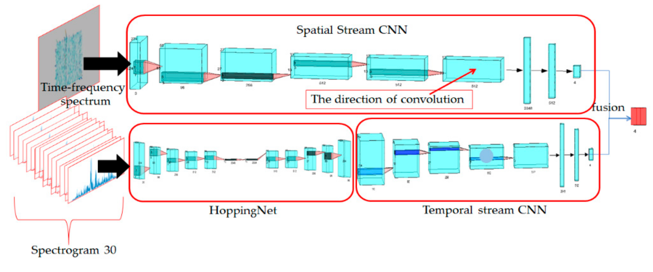
Because the workpiece we detect is mainly constructed from powder metallurgy, most module patterns do not turn into faults over their lifetime, but they can cause several conditions that affect the user’s using perception [32]. We divide the inspected workpiece into four categories: normal, low, noise, and collision. It is hard to make a reasonable quality standard for various devoted companies for a stepper motor with four models.
The artifacts with normal sound defined by the quality control team in combination with the data characteristics will also have some differences due to the heterogeneity of the complex system, but the overall sound signal characteristics are stable. Although there are no obvious defects in the workpiece, the damping of the whole system will be increased due to the deformation of the shaft and gear. However, this kind of condition will not affect the service life of the complete system. We define the workpiece that cannot produce a mechanical sound of normal value as low sound. Due to the whole lifting mechanism in the operation process needing a certain transmission sound, users with good sense of hearing and touch are brought into the process of using the product (such as a telescopic camera). The vibrating sound with damping can be recognized with less energy through the bionic ear, which is similar to the auditory characteristics of a human ear. This kind of pattern will not cause faults, but it will have a great impact on people’s usage impression. Most of the workpiece is made of metal sintering with a rough surface, and the particles will fall off in the process of use. This type of module will not be further converted into a fault, but the effect on human auditory perception is very large, so we classify this kind of module as a noisy workpiece. The workpiece with low noise and low sound can be mixed into the finished product in a certain proportion to form product categories of different quality control standards. As mentioned above, because the gears are made of powder metallurgy, the complexity of defects leads to different collision sounds. The hopping information and the overall information in the whole operation cycle are still different from the data of the normal module. All of the data are screened by the quality control team combined with the data analysis method. In the process of using the system, this kind of defect will be upgraded to failure with high probability. However, the intermittent bad sound signal caused by it has little impact on the human ear, so we unified it into a kind of module that may cause faults. This kind of product is strictly controlled and is not allowed to be mixed in the product that has passed the quality control inspection.
Currently, stepper motors and variable speed modules are manually placed on test platforms by operators to determine whether or not a defective voice is overheard. In particular, it is difficult to reach a consensus among multiple enterprises regarding which workpiece affects people’s subjective perception because the quality cannot be objectively evaluated, resulting in a large number of economic losses and many disputes. As previously stated, defect detection and quality control for stepper motors and variable speed modules are achieved by employees listening to the sound repeatedly in a closed silent room to identify the pattern type. Then, the analyzed defect is inspected by experienced staff. This method of detection is not only costly, but also inefficient, and it fluctuates with the flow of employees. Observation based on staff experience to achieve defect detection leads to various disadvantages, such as time consumption and a lack of real standardization.
Therefore, a pattern evaluation system based on anthropomorphic perception is urgently needed. The perception system of human can be divided into two branches: ventral and dorsal flow. Ventral flow represents people’s perception of the overall state of events, and dorsal flow represents the perception of transient fluctuations, by spatial stream and temporal stream CNNs, respectively. In the T-CNN stream, we used a fully convolutional neural network to extract the detailed features of the hoppings between each time spectrum. In order to be more similar to the human perception system, we proposed a neural network model with two different functional branches to identify signals [33]. The characteristics of the system’s bionic ear are similar to human ears, and the calibration dataset is screened by multi-party quality control personnel combined with PCA [34]. After using PCA, we selected a workpiece with obvious features of 14 dimensions to identify, classify, and match with experienced workers, so as to obtain a dataset of the network. With a large amount of calibrated data, the training model has higher objectivity than single subjective discrimination.
To address these problems, we designed a new set of analysis period testing and load conditions for devices as well as matching discriminating procedures. According to the customary distance of using smartphones, we wanted to determine the position where the sound is the strongest and the loss is the least. We placed the bionic ear and two other sets of sensors of the same type on the envelope sphere with a radius of 10 cm and selected the right end of the test module as the optimal sound acquisition location. In the experiments, the sensor we used was an acoustic pressure test capacitor microphone AWA14424D, matched with an AWA6162 cochlear implant and AWA14604C bionic auricle. Figure 1 shows the detailed anatomy of the stepper motor module and the measurement environment.
Due to needing to determine the detailed sound features, we entered sound information at different time periods in the identification system. The system acquisition software was LabVIEW 2018, which uses serial port communication with the stepper motor control card for conducting segmented periodic acquisition. The software system was programmed in Python 3.7. The detection algorithm was developed by OpenCV and TensorFlow 1.5 deep learning platform. Figure 2 shows the device composition of our entire system.

3. Proposed Method

Figure 3 provides an overview of the processing workflow, which displays the components of our proposed vision system. Our system can be roughly divided into two parts: ventral flow and dorsal flow. In the spatial stream CNN, the time-frequency spectrum is decomposed into a 128 high-dimensional feature graph and sent to the directional convolution layer for feature extraction. The global features contained in different time spectrums, which are the normal and missing reducer modules, are identified by directional convolution. The sound of the defective module causes sensory discomfort for people. In another channel, the hopping information of spectral signals is also decomposed into 512 high-dimensional features, and the hopping feature graph is generated and put into a temporal stream for identification.
Considering that the system is not a single detection of possible defects, the main purpose was to identify the characteristic workpiece data determined by the quality control team and us after decomposition of features by the contribution matrix in PCA in a way similar to human perception. Therefore, we divided the system into two parts to learn different data, and finally fused the two branches of loss functions in the way described above, which contains two major parts: the S-CNN and the temporal stream CNN and HoppingNet. The temporal stream CNN and HoppingNet module mainly imitate people’s perception of transient signals to identify the hopping detail features between multiple spectrums in the corresponding time spectrum. The spatial stream CNN detection was developed only to identify whether the global time-frequency spectrum feature graph in the whole test process contained defective information. Finally, we used a weighted sum to fuse the recognized scores. As shown in Figure 3, the temporal stream CNN and HoppingNet module can be divided into four steps: feature extraction, direction convolution, output, and fusion layer.
The input of this system is a time-frequency spectrum diagram of 30 time spectrum diagrams generated in the whole step resistance module running completely in a period of progressive operation under the condition of loaded 480 g, and input two branches in the form of images.
We provide the theoretical background for the model in Section 2.
We briefly describe the details of our algorithm in Section 3.1, the database processed in our work in Section 3.2 and Section 3.3. Finally, the experimental details are shown in Section 3.4.

3.1. Branch of Temporal Stream CNN and HoppingNet

3.1.1. HoppingNet

The method of extracting high-dimensional features by a CNN network has some limitations. The labels of optical flow diagrams produced by traditional methods have errors of dynamic intention, so their prediction quality is also limited.
We used the optical flow program to generate the hopping features of time spectrums, as the goal of a network is to learn the residuals [35] between the spectrums. Pre-trained HoppingNet without a full connection layer can quickly extract features and meet the requirement of multi-frame input speed of temporal stream CNN. We used an unsupervised learning and pre-trained fully convolutional neural network (FCN) network to predict the features of the time spectrum hopping characteristics. We removed the feature graph of the last full convolution segmentation layer and cascaded it with the T-CNN network, which clusters features into the cascade action identification network. Because the full convolution network structure can be regarded as an image reconstruction system, each scale contains information about different importance.
Figure 4 shows the basic structure of HoppingNet, which composed of coding, bridge, and decoding blocks.
The general structure of HoppingNet is shown in Table 1.
Here, we use three groups of loss functions to represent the learning effect of the time spectrum hopping learning network, and these loss functions are as follows.
The reconstruction loss function, which is calculated as:
L pixel = 1 hw i h j w ρ I 1 i , j I 2 i + V i , j x , j + V i , j y
where i,j represent the values in the horizontal and vertical coordinates of the pixels in the time spectrum diagram I, and V x and V y are the estimated spectrum hopping in the horizontal and vertical directions. To reduce the influence of outliers, we used the Charbonnier penalty ρ x = x 2 + ϵ 2 α where h and ω are the height and width of spectrums ( I 1   and   I 2 ).
Because most of the spectrum hopping will cause the non-closed interval, we used smoothness loss to deal with the aperture problem that causes ambiguity in estimating hopping features in non-textured regions. It is calculated as:
L smooth = ρ V x x + ρ V y x + ρ V x y + ρ V y y
where V x x and V y x are the gradients of the estimated hopping V x in each direction, and V x y and V y y are the same as V y .
In order to test the learning ability of network reconstruction, I is used here to compare the feature graph after network reconstruction with the run-out feature generated by the original input graph by means of X. For this similarity evaluation, we use a comparison parameter to evaluate the reconstruction quality. SSIM represents the structural similarity between the target and the predicted image.
SSIM I p 1 , I p 2 = 2 μ p 1 μ p 2 + c 1 2 σ p 1 p 2 + c 2 μ p 1 2 + μ p 2 2 + c 1 σ p 1 2 + σ p 2 2 + c 2
where μ p 1 and μ p 2 are the mean value of input spectrums, σ p 1 and σ p 2 are the variance of spectrums, and σ p 1 p 2 is the covariance of these inputs. c 1 and c 1 are constants to stabilize division by a small denominator, which are 0.0001 and 0.001, respectively.
L ssim = 1 N n N 1 SSIM I 1 n , I 1 n
We divided the whole picture into 6 × 6 regions, traversing with a stride length of 6. N is the number of pixel points in each region. By comparing the characteristic graphs I 1 n and I 1 n before and after the partition reconstruction, we know the learning status of the spectrum hopping information of the network.
Finally, we combined several loss functions to form an end-to-end training objective function.
L S = L pixel + L smooth + L ssim
Unsupervised pre-training networks are more primitive to high-dimensional features and can guarantee the initial generalization ability of model learning. In order to increase the learning ability of the time spectrum hopping characteristics, we defined the contrasting feature colors to represent the hopping feature. Finally, the way to fuse the network is to refer to article [36], and we achieved good results in terms of accuracy. Figure 5 shows the true graphs and prediction feature graphs of spectrum hopping feature recognition. To increase the contrast to graphs, we turned black the background.

3.1.2. Temporal Stream CNN

The features generated by HoppingNet will feed into temporal stream CNN after 30 frames have been extracted. The function of this structure is to learn the correlation of information of features in the time-dimension. The general structure of the network is shown in Table 2. The final full connection layer neuron returns the model’s probability distribution using softmax, and the classification of our model is four. Finally, we combined this probability with the results of spatial stream.

3.2. The Branch of Spatial Stream CNN

Because the time-frequency spectrum is the superposition of the time spectrum in the time-dimension, the model is required to learn the high-dimensional features of correlated pixels rather than single adjacent pixels. Therefore, we use the S-CNNs structure that can recognize spatial information to learn the pixels of the spatial connection between the spectrums.
In traditional CNN, any layer receives data from the upper layer for input, and then performs convolution and activation on the next layer. This process is performed in sequence. Similarly, S-CNN also regards the rows or columns of feature maps as a layer and uses convolution plus nonlinear activation to realize deep neural network in space. S-CNN extends the deep convolutional neural network to a rich spatial level. This enables spatial information to spread on the same layer of neurons and enhances the spatial information, which is particularly effective for identifying structured objects.
The four-direction convolution extracts high-dimensional features from the CNN structure, extracts information between layers of pixels, and finally inputs them into the recognition layer. As shown in Figure 6, the spatial information of the time-frequency spectrum is extracted from the high-dimensional feature map extracted by the CNN, and the correlation between the pixel is mapped in the space along with four different directions. Finally, it summarizes it in another high-dimensional feature layer. A simplified version of spatial stream CNN can be composed of the following four parts:
  • Feature extraction: the high-dimensional features layer of the CNN network contains rich spatial relationships. It uses 512 high-dimensional channels to replace the traditional RGB 3-channel input. The first four convolution structures of the spatial stream CNN are the same as shown in Table 1.
  • Direction convolution: the direction convolution extracts pixel correlation information of different directions from the high-dimensional features layer with width (W) of 128, height (H) of 128, and 256 channels (C) in four directions: downward, upward, right, and left. The direction convolution kernel size is 3 × 3, and all pieces share a set of convolution kernels. Directional convolution not only mentions the high-dimensional features between adjacent pixels, but also learns the spatial relations between distant pixels, so that time-frequency spectrum features in the whole-time domain can be perceived. The nonlinear activation function rectified linear units (ReLU) has become the most widely used activation function because it can effectively prevent the gradient from disappearing and accelerate the convergence speed during the training process. All slices share a set of convolution kernels, so the structure is similar to the RNN structure. The convolution information in the previous slice is transferred to the next slice, and the mathematical transformation between each input value X and its output X’ can be formulated as:
    X i , j , k = X i , j , k j = 1 X i , j , k + f m n X m , j 1 , k + n 1 × K m , i , n ) , j = 2 , 3 , , H
    where X’ is a three-dimensional tensor, and the convolution direction is alone with four directions. j represents the number of convolutions from the position at the beginning of the direction, and i,k, respectively, represent the number of layers in the direction of the convolution and the position of the convolutional slice in the same layer. When j is equal to different values (except when it is equal to 1), i,k are the number of slices in different directions. In the above way, the weights in the tensor will be adjusted between different directions in the high-dimensional space to realize the correlation of the details of each position.
  • 3.
    Output: this block is consist of three fully connection layers.
    4.
    Fusion: we fuse two streams’ scores with a spatial to temporal stream ratio of 1:1.5.

    3.3. Model Implementation

    We used the same type of sensor group to compare the sound signals on the same envelope, and get the direction of the strongest signal. In terms of hardware, the bionic ear sensor simulates the cochlea and auricle structure of human beings. In terms of software, it adjusts the distribution characteristics of input signals by using the Mel spectrum [37] and A-weight [38] method to process signals. It obtains signal extraction parameters similar to the auditory perception curve of human ears.
    Figure 7 shows the pictures of different workpieces and their corresponding time-frequency spectrum characteristic pictures. The red circle represents the unstable surface, broken gear, and litter generated by sintering, which will interfere with the operational of the whole system. Figure 8 shows one of the main patterns we identified, artifacts with noisy sound, which do not cause faults but seriously affect the human senses.
    All patterns in this paper do not refer to a single mechanical defect, but to the patterns that make people feel uncomfortable. Since the workpiece in the deceleration module was formed by powder metallurgy technology, it was difficult to analyze and form a single fault test group. Therefore, we directly used sensory characteristics to group the tested samples. Fusing with the edge detection results, which makes the above characteristics easy to find, we can figure out what kind of pattern of the artifact affects people.
    These definitions were put forward by the quality control team. The system aims to detect the workpiece that is disturbing to the human senses. Most patterns will not be converted or broken like traditional mechanical defects, which directly affect the user experience. In order to make the discriminant perception of the system to be closer to human beings, we used the contribution matrix in PCA to reduce the discriminant feature dimension when screening data, and classified the workpiece together with experienced quality control workers. We extracted the 14 dimensional features including three-layer wavelet packet entropy, time-domain signal kurtosis, time-domain signal average variance, a decibel value after weighting, time-domain signal root mean square (RMS), a Hilbert envelope characteristic value, frequency-domain signal peak width, frequency-domain signal energy and time-domain signal kurtosis, time-domain signal slanting degrees, time-domain signal margin, index of time-domain signal pulse, and frequency-domain power spectrum.
    Finally, as shown in Table 3, after the analysis of more than 13,000 workpieces, we determined the five dimensions of PCA as the discriminating quantity, and distinguished four major types of defective workpieces.
    It can be seen from Table 3 that the contribution matrix reaches an inflection point when the feature dimensions are reduced to five dimensions, so we chose the five-dimensional PCA components with higher efficiency to classify the data. When screening data, we took 10 full cycles for analysis at the sampling rate of 10 kHz, and we only selected the workpieces that were clearly identified by experienced workers for classification.
    Experimental results show that the model trained by pre-screened data has faster convergence and higher accuracy than that trained by original and unscreened feature signals. It can be seen from Figure 7 that the tagged data have low noise, relatively clear time-frequency spectrum characteristics, and spectrum hopping characteristics. The experimental results show that the model of data training is more robust.
    Through this anthropomorphic fusion recognition system, the inspection task of the front-end module has been completed. The system will directly judge whether the product is bad if there are any defects identified. By training the clearly calibrated data, we can identify various types of patterns classification, and overcome the problem that patterns cannot be analyzed objectively by humans.

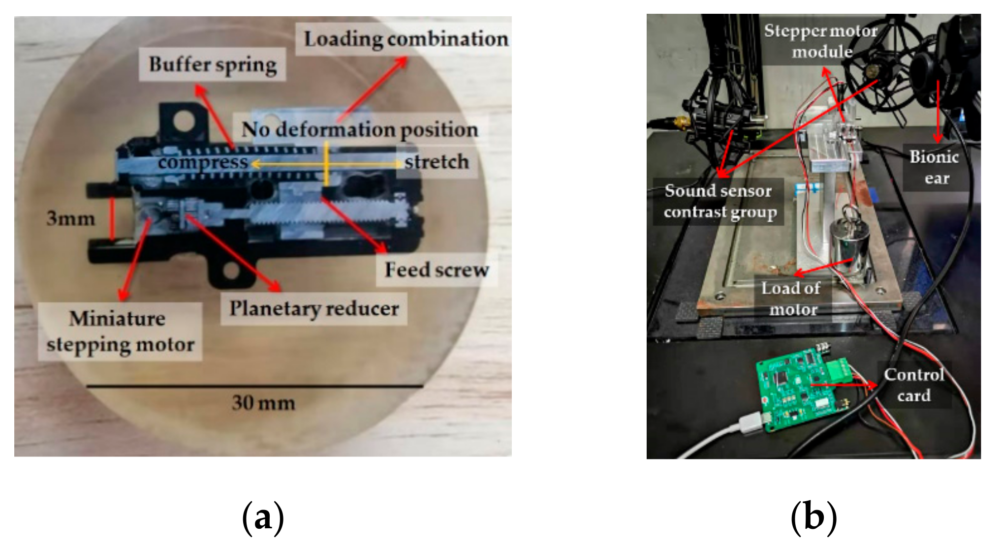
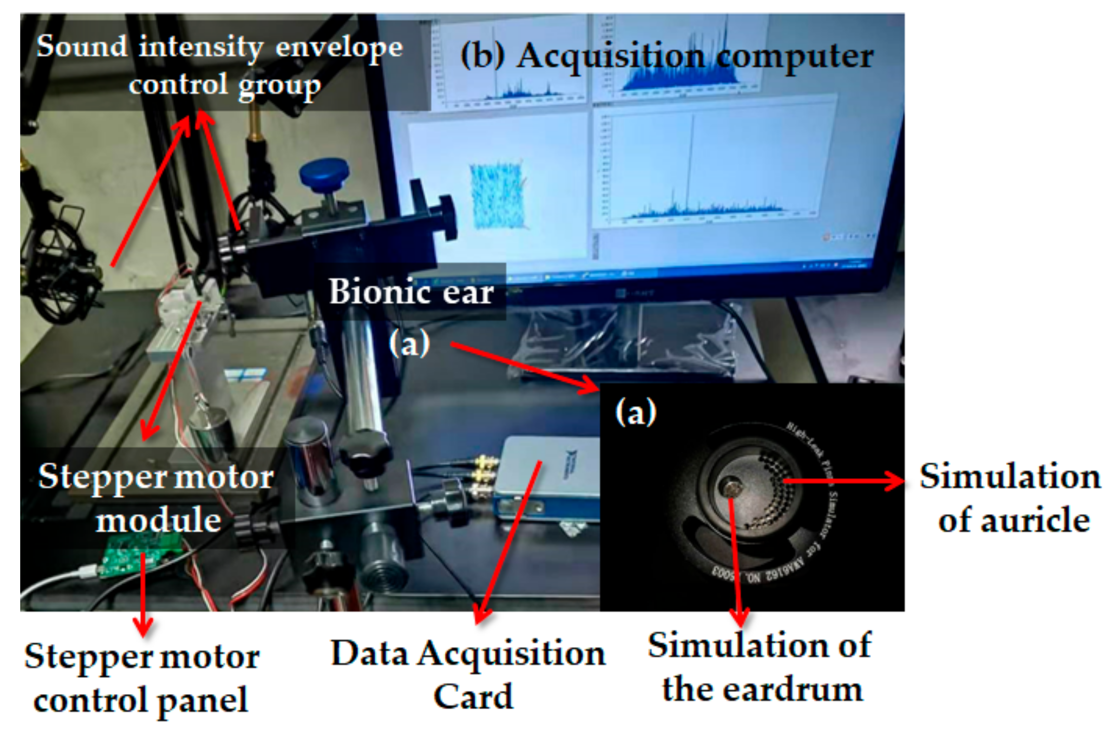
    3.4. Experiment Details

    3.4.1. The Dataset

    In this paper, our dataset was collected by the device shown in Figure 2, and we evaluated our method on this dataset, shown in Figure 9 and Figure 10. In order to match the spectrum with the corresponding time-frequency spectrum, we set the sample rate as 10 kHz. We generated spectrum of discrete Fourier transform (DFT) for every 0.2 s signal, and for every 2000 pieces of data collected in the spectrum window [39]. A total of 6 s are used for the operation of the module, so a time-frequency spectrum corresponds to 30 spectrum graphs and 15 hopping characteristic graphs. Through continuous learning of jump variables, we removed the feature graph of the last full convolution label and cascaded it with the T-CNN network. All data were normalized in order to search for generic characteristics. The pattern of the workpiece was divided into four categories, and the input images were all 256 × 256. Data corresponding to the structure of our model can be divided into two parts: the overall characteristics of the time-frequency spectrum and time spectrum flow with the hopping characteristics.
    During the entire test cycle, a 480 g load was applied to the system to detect the strength of the powder molded gear set in the module. The detection is divided into three main steps: lowering, lifting, and interfering collision.
    In the corresponding time-frequency spectrum diagram, we adopted normalized clear color discrimination, as described in Figure 10. We used 4325 positive samples and 9245 negative samples. Through PCA and with experienced workers working together, we distinguished and collected data of the sample workpiece with four kinds of relatively clear patterns. Figure 10 shows the 3D time-frequency spectrum images of different kinds of artifacts.

    3.4.2. The Implementation Process

    Our model was trained on one NVIDIA 4 GTX2080 GPUs with 16 GB memory for roughly 10 h. Experiments were implemented based on the deep learning framework TensorFlow. The operating system was Windows 10.
    The input image size of the spectrum is 224 × 224, which is cropped from the original 256 random jitter. The hopping characteristics identification network is a total convolutional neural network, which identifies the hopping features of 30 spectral graphs as high-dimensional features of 128 dimensions and sends them into the time network. The time network consists of five convolution layers and three FC layers, and the final softmax score is calculated by using the average score. The spatial CNN network proved its powerful ability in image detection with the spatial relationships, while the structure of spatial CNN is very complex and has complex directional convolution, which is a kind of black-box operation for us. In order to prevent overfitting, we enhanced the training data and, with random horizontal flipping and RGB jittering, adjusted the exposure curve.
    Similar results were also achieved by Alex-net and Resnet-101 [40]. We speculate that the reason for the failure is that with multiple feature extraction, the network extracts more representative information and naturally loses detail. However, in some cases, the differences between bad products and good products in our data lie in small changes. For some pictures, even people can be wrong. Therefore, we only use artifacts that can clearly distinguish features, and the fusion of multiple defect features is given to the neural network to fit by itself. According to the appeal, we conducted pre-training for the spatial network and run-out signal detection network. The difference is that the spatial network adopts supervised pre-training and the run-out signals detection network adopts unsupervised pre-training to increase the normality and sensitivity of signal recognition. The method did work and the accuracy was improved to 96.1%, but it was still too low for our demand. In this case, we used the continuous finetuning mechanism to further improve the accuracy, but only the action categorical loss function was computed. In spatial net training, a 224 × 224 sub-image is randomly cropped from the selected frame, then undergoes random horizontal flipping and RGB jittering. The sub-image is sampled from the whole frame, not just from its 256 × 256 center. In temporal net training, we computed an optical flow volume I for the selected training frame, as described in Section 3. From that volume, a fixed-size 224 × 224 × 2 L input is randomly cropped and flipped. For FC layers, the weight parameters are initialized from a truncated random normal distribution subject to N ~ (0, 2 n ), where n denotes the number of connections between two layers. In order to prevent the network from overfitting, we adopted a mirror to augment the data. The data sample was expanded fivefold by using the above method.
    In our case, a network architecture of two tributaries were modified so that it had two softmax classification layers on top of the last fully connected fusion layer. One softmax layer computes global feature scores, and the other one computes the local hopping characteristic scores. Each layer is equipped with its own loss function coming from the respective dataset. For each workpiece, we made the corresponding time-frequency spectrum graph and 15 hopping characteristic graphs generated by 30 frames of the spectrum. The overall training loss is computed as the sum of the individual tasks’ losses, and the network weight derivatives can be found by back-propagation. We selected the cross-entropy function as the overall loss function of our model. During the training process, the stochastic gradient descent (SGD, momentum = 0.9) with mini-batches of weight samples was applied to update the weight parameters. When we trained one branch, we froze the weight of the other branch, until the performance was stable, and we carried out the whole weight training. Temporal and spatial streams are complementary, as their fusion significantly improves on both. The learning rate is initially set to 10−2, and then decreased according to a fixed schedule. The rate is changed to 10−3 after 30 K iterations, then to 10−4 after 50 K iterations, and stopped after 60 K iterations.

    4. Results

    In our system, similarity to human perception is the evaluation criterion of system performance. Here, we worked with the staff of a professional QC group to get the accuracy. The formula for calculating the accuracy is defined by Equation (7). To evaluate the performance of our method, we validated our module on a dataset and achieved the final detection accuracy of 96.1%. Through a confusion matrix, we obtained the accuracy and recall rate of the system, and passed the comparison test of the production QC group. Table 4 shows the performance of the model under different augmentation methods of input data and parameters.
    We fused the softmax scores of the two branches at a ratio of 1:1.5. Finally, the overall loss was used to carry out fine-tune [41] the trained network, and high accuracy was obtained. The experiment shows that our model has the ability to distinguish defect-free and defective images in our dataset and achieve higher accuracy than others, which proves the effectiveness of our two-stream module. In Table 5, we compared the results of several other models with identifying local features and global features in the operating status of the stepper motor.
    The detection results of our model on the four kinds of samples are shown in Figure 11. In the process of training, we used the method of classification weights in the final layer to solve the problem of the unbalanced data set. As our content involved the perception of good and bad samples, the accuracy of this model is constituted by true-positive (TP), true-negative (TN), false-positive (FP), and false-negative (FN) values by.
    Accuracy = T P + T N T P + T N + F P + F N

    5. Conclusions

    In this study, we adopted a two branch (spatial stream and temporal stream) concatenated HoppingNet to simulate the ventral and dorsal flow system of the human perception system. We used the bionic ear to recognize the sound; the signal characteristics were more consistent with the sensitivity of the human ear and could simulate the sound echo of the cochlea. What we identified in the dataset of the system and what differentiates it from other models is that defective artifacts are not defined as a particular kind of mechanical or electrical fault, but also as individuals that adversely affect human perception. We used PCA to subdivide the dataset along with experienced quality control team members, making the perception characteristics of the intelligent system very close to the humans. We added a batch normalization (BN) layer at the end, because the network would not converge well when overall training was carried out. After many experiments, our end-to-end system finally achieved very good results. The accuracy and objectivity of the analysis are far better than those of a single person in the quality control team.
    Our research shows that the deep learning model could replace the human perception system to complete a series of industrial detection under certain hardware conditions.
    However, there are still many difficulties in our approach, such as the high cost of dataset production and too many training model parameters. In the future, we hope to make more lightweight sensing models in the field of industrial testing to improve the efficiency of production.

    Author Contributions

    X.F. did the main work; project administration, J.W.; resources, H.F.; Z.F. and L.Z. completed the experiments. All authors have read and agreed to the published version of the manuscript.

    Funding

    This research was funded by [the platform Chinese Sichuan Provincial Science and Technology Department Key Research and Development fund] grant number [2019YFG0356] and [the fundamental Research Funds for the Sichuan University] grant number [2018GZDZX0015]. And the APC was funded by [Sichuan University].

    Acknowledgments

    This work is partially supported by the Intelligent Manufacturing Project, and the platform Chinese Sichuan Provincial Science and Technology Department Key Research and Development fund, the fundamental Research Funds for the Sichuan Universities (2019YFG0356) and (2018GZDZX0015). This research received no external funding from the fundamental Research Funds for the Sichuan Universities, grant number [2019YFG0356] and (2018GZDZX0015). The APC was funded by [Sichuan Universities].

    Conflicts of Interest

    The authors declare no conflict of interest.

    References

    1. Junoh, A.K.; Nopiah, Z.M.; Muhamad, W.Z.W.; Nor, M.J.M.; Fouladi, M.H. An Optimization Model of Noise and Vibration in Passenger Car Cabin. Adv. Mater. Res. Switz. 2012, 383, 6704–6709. [Google Scholar] [CrossRef]
    2. Albert, B.; Zanni-Merk, C.; de Beuvron, F.D.B.; Maire, J.L.; Pillet, M.; Charrier, J.; Charrier, J.; Knecht, C.A. Smart System for Haptic Quality Control Introducing an Ontological Representation of Sensory Perception Knowledge. In Proceedings of the 8th International Joint Conference on Knowledge Discovery, Knowledge Engineering And Knowledge Management, Porto, Portugal, 9 November 2016; pp. 21–30. [Google Scholar]
    3. Koch, C.; Georgieva, K.; Kasi eddy, V.; Akinci, B.; Fieguth, P. A review on computer vision based defect detection and condition assessment of concrete and asphalt civil infrastructure. Adv. Eng. Inform. 2015, 29, 196–210. [Google Scholar] [CrossRef] [Green Version]
    4. Jian, C.X.; Gao, J.; Ao, Y.H. Automatic surface defect detection for mobile phone screen glass based on machine vision. Appl. Soft Comput. 2017, 52, 348–358. [Google Scholar] [CrossRef]
    5. Park, J.K.; Kwon, B.K.; Park, J.H.; Kang, D.J. Machine Learning-Based Imaging System for Surface Defect Inspection. Int. J. Precis. Eng. Manuf. Green. Technol. 2016, 3, 303–310. [Google Scholar] [CrossRef]
    6. Shanmugamani, R.; Sadique, M.; Ramamoorthy, B. Detection and classification of surface defects of gun barrels using computer vision and machine learning. Measurement 2015, 60, 222–230. [Google Scholar] [CrossRef]
    7. Cipollini, F.; Oneto, L.; Coraddu, A.; Savio, S.; Anguita, D. Unintrusive Monitoring of Induction Motors Bearings via Deep Learning on Stator Currents. Procedia Comput. Sci. 2018, 144, 42–51. [Google Scholar] [CrossRef]
    8. Li, C.; Sanchez, R.V.; Zurita, G.; Cerrada, M.; Cabrera, D. Fault Diagnosis for Rotating Machinery Using Vibration Measurement Deep Statistical Feature Learning. Sensors 2016, 16, 895. [Google Scholar] [CrossRef] [PubMed] [Green Version]
    9. Yao, Y.; Wang, H.L.; Li, S.B.; Liu, Z.H.; Gui, G.; Dan, Y.B.; Hu, J.J. End-To-End Convolutional Neural Network Model for Gear Fault Diagnosis Based on Sound Signals. Appl. Sci. 2018, 8, 1584. [Google Scholar] [CrossRef] [Green Version]
    10. Wang, J.L.; Yang, Z.L.; Zhang, J.; Zhang, Q.H.; Chien, W.T.K. AdaBalGAN: An Improved Generative Adversarial Network with Imbalanced Learning for Wafer Defective Pattern Recognition. IEEE Trans. Semiconduct. Manuf. 2019, 32, 310–319. [Google Scholar] [CrossRef]
    11. Wang, L.M.; Qiao, Y.; Tang, X.O. Action Recognition with Trajectory-Pooled Deep-Convolutional Descriptors. In Proceedings of the IEEE Conference on Computer Vision and Pattern Recognition (CVPR), Boston, MA, USA, 8 June 2015; pp. 4305–4314. [Google Scholar]
    12. Gan, M.; Wang, C.; Zhu, C.A. Construction of hierarchical diagnosis network based on deep learning and its application in the fault pattern recognition of rolling element bearings. Mech. Syst. Signal Process. 2016, 72, 92–104. [Google Scholar] [CrossRef]
    13. Shang, C.; Yang, F.; Huang, D.X.; Lyu, W.X. Data-driven soft sensor development based on deep learning technique. J. Process Control 2014, 24, 223–233. [Google Scholar] [CrossRef]
    14. Yao, L.; Ge, Z.Q. Deep Learning of Semisupervised Process Data with Hierarchical Extreme Learning Machine and Soft Sensor Application. IEEE Trans. Ind. Electron. 2018, 65, 1490–1498. [Google Scholar] [CrossRef]
    15. He, K.M.; Gkioxari, G.; Dollar, P.; Girshick, R. Mask R-CNN. In Proceedings of the IEEE International Conference on Computer Vision, Venice, Italy, 22 October 2017; pp. 2980–2988. [Google Scholar]
    16. Le, T.D.; Huynh, D.T.; Pham, H.V. Efficient Human-Robot Interaction using Deep Learning with Mask R-CNN: Detection, Recognition, Tracking and Segmentation. Int. Conf. Control, Autom. Robot. Vis. 2018, 162–167. [Google Scholar]
    17. Pobar, M.; Ivasic-Kos, M. Mask R-CNN and Optical flow based method for detection and marking of handball actions. In Proceedings of the 2018 11th International Congress on Image and Signal Processing, Biomedical Engineering and Informatics (Cisp-Bmei 2018), Beijing, China, 13–15 October 2018. [Google Scholar]
    18. Fang, X.; Jie, W.; Feng, T. An Industrial Micro-Defect Diagnosis System via Intelligent Segmentation Region. Sensors 2019, 19, 2636. [Google Scholar] [CrossRef] [Green Version]
    19. Zhang, J.C.; Zhang, Y.; Ji, D.H.; Liu, M.C. Multi-task and multi-view training for end-to-end relation extraction. Neurocomputing 2019, 364, 245–253. [Google Scholar] [CrossRef]
    20. Kang, G.Q.; Gao, S.B.; Yu, L.; Zhang, D.K. Deep Architecture for High-Speed Railway Insulator Surface Defect Detection: Denoising Autoencoder With Multitask Learning. IEEE Trans. Instrum. Meas. 2019, 68, 2679–2690. [Google Scholar] [CrossRef]
    21. Hu, C.; Tang, X.L.; Zou, L.; Yang, K.; Li, Y.N.; Zheng, L. Numerical and Experimental Investigations of Noise and Vibration Characteristics for a Dual-Motor Hybrid Electric Vehicle. IEEE Access 2019, 7, 77052–77062. [Google Scholar] [CrossRef]
    22. Kwon, Y.H.; Shin, S.B.; Kim, S.D. Electroencephalography Based Fusion Two-Dimensional (2D)-Convolution Neural Networks (CNN) Model for Emotion Recognition System. Sensors 2018, 18, 1383. [Google Scholar] [CrossRef] [PubMed] [Green Version]
    23. Chen, C.L.P.; Liu, Z.L. Broad Learning System: An Effective and Efficient Incremental Learning System without the Need for Deep Architecture. IEEE Trans. Neural Netw. Learn. Syst. 2018, 29, 10–24. [Google Scholar] [CrossRef] [PubMed]
    24. Salamon, J.; Bello, J.P. Deep Convolutional Neural Networks and Data Augmentation for Environmental Sound Classification. IEEE Signal Process. Lett. 2017, 24, 279–283. [Google Scholar] [CrossRef]
    25. Mehta, R.K.; Parasuraman, R. Neuroergonomics: A review of applications to physical and cognitive work. Front. Hum. Neurosci. 2013, 7, 889. [Google Scholar] [CrossRef] [PubMed] [Green Version]
    26. Feichtenhofer, C.; Pinz, A.; Zisserman, A. Convolutional Two-Stream Network Fusion for Video Action Recognition. In Proceedings of the IEEE Conference on Computer Vision and Pattern Recognition, Las Vegas, NV, USA, 26 June 2016; pp. 1933–1941. [Google Scholar]
    27. Du, Y.; Wang, W.; Wang, H. Hierarchical Recurrent Neural Network for Skeleton Based Action Recognition. In Proceedings of the IEEE Conference on Computer Vision and Pattern Recognition, Boston, MA, USA, 8 June 2015; pp. 1110–1118. [Google Scholar]
    28. Chen, Y.H.; Emer, J.; Sze, V. Eyeriss: A Spatial Architecture for Energy-Efficient Dataflow for Convolutional Neural Networks. In ACM SIGARCH Computer Architecture News; IEEE Press: Piscataway, NJ, USA, 2016; pp. 367–379. [Google Scholar]
    29. Fu, G.; Liu, C.J.; Zhou, R.; Sun, T.; Zhang, Q.J. Classification for High Resolution Remote Sensing Imagery Using a Fully Convolutional Network. Remote Sens. 2017, 9, 498. [Google Scholar] [CrossRef] [Green Version]
    30. Gong, M.G.; Zhang, M.Y.; Yuan, Y. Unsupervised Band Selection Based on Evolutionary Multiobjective Optimization for Hyperspectral Images. IEEE Trans. Geosci. Remote Sens. 2016, 54, 544–557. [Google Scholar] [CrossRef]
    31. Chan, T.H.; Jia, K. PCANet: A Simple Deep Learning Baseline for Image Classification. IEEE Trans. Image Process. 2015, 24, 5017–5032. [Google Scholar] [CrossRef] [PubMed] [Green Version]
    32. Wang, F.; Zhang, J.; Xu, X.; Cai, Y.F.; Zhou, Z.G.; Sun, X.Q. New teeth surface and back (TSB) modification method for transient torsional vibration suppression of planetary gear powertrain for an electric vehicle. Mech. Mach. Theory 2019, 140, 520–537. [Google Scholar] [CrossRef]
    33. Bo, H.; Hualong, H.; Hongtao, L. Convolutional Gated Recurrent Units Fusion for Video Action Recognition. In Proceedings of the 24th International Conference on Neural Information Processing, ICONIP, Guangzhou, China, 14 November 2017. [Google Scholar]
    34. Mnassri, B.; El Adel, E.; Ouladsine, M. Reconstruction-based contribution approaches for improved fault diagnosis using principal component analysis. J. Process. Control 2015, 33, 60–76. [Google Scholar] [CrossRef]
    35. Zhang, K.; Zuo, W.M. Beyond a Gaussian Denoiser: Residual Learning of Deep CNN for Image Denoising. IEEE Trans. Image Process. 2017, 7, 3142–3155. [Google Scholar] [CrossRef] [Green Version]
    36. Tu, Z.G.; Xie, W.; Qin, Q.Q.; Poppe, R.; Veltkamp, R.C.; Li, B.X.; Yuan, J.S. Multi-stream CNN: Learning representations based on human-related regions for action recognition. Pattern Recognit. 2018, 79, 32–43. [Google Scholar] [CrossRef]
    37. Benisty, H.; Malah, D.; Crammer, K. Grid-based approximation for voice conversion in low resource environments. EURASIP J. Audio Speech Music Process. 2016, 3, 1–14. [Google Scholar] [CrossRef] [Green Version]
    38. Torija, A.J.; Ruiz, D.P.; Ramos-Ridao, A.F. Use of back-propagation neural networks to predict both level and temporal-spectral composition of sound pressure in urban sound environments. Build. Environ. 2012, 52, 45–56. [Google Scholar] [CrossRef]
    39. Kulin, M.; Kazaz, T.; Moerman, I.; De Poorter, E. End-to-End Learning From Spectrum Data A Deep Learning Approach for Wireless Signal Identification in Spectrum Monitoring Applications. IEEE Access 2018, 6, 18484–18501. [Google Scholar] [CrossRef]
    40. Szegedy, C.; Ioffe, S.; Vanhoucke, V.; Alemi, A.A. Inception-v4, Inception-ResNet and the Impact of Residual Connections on Learning. In Proceedings of the Thirty-First Aaai Conference on Artificial Intelligence, San Francisco, CA, USA, 4 February 2017; pp. 4278–4284. [Google Scholar]
    41. Tajbakhsh, N.; Shin, J.Y.; Gurudu, S.R.; Hurst, R.T. Convolutional Neural Networks for Medical Image Analysis: Full Training or Fine Tuning? IEEE Trans. Med Imaging 2016, 5, 1299–1312. [Google Scholar] [CrossRef] [PubMed] [Green Version]
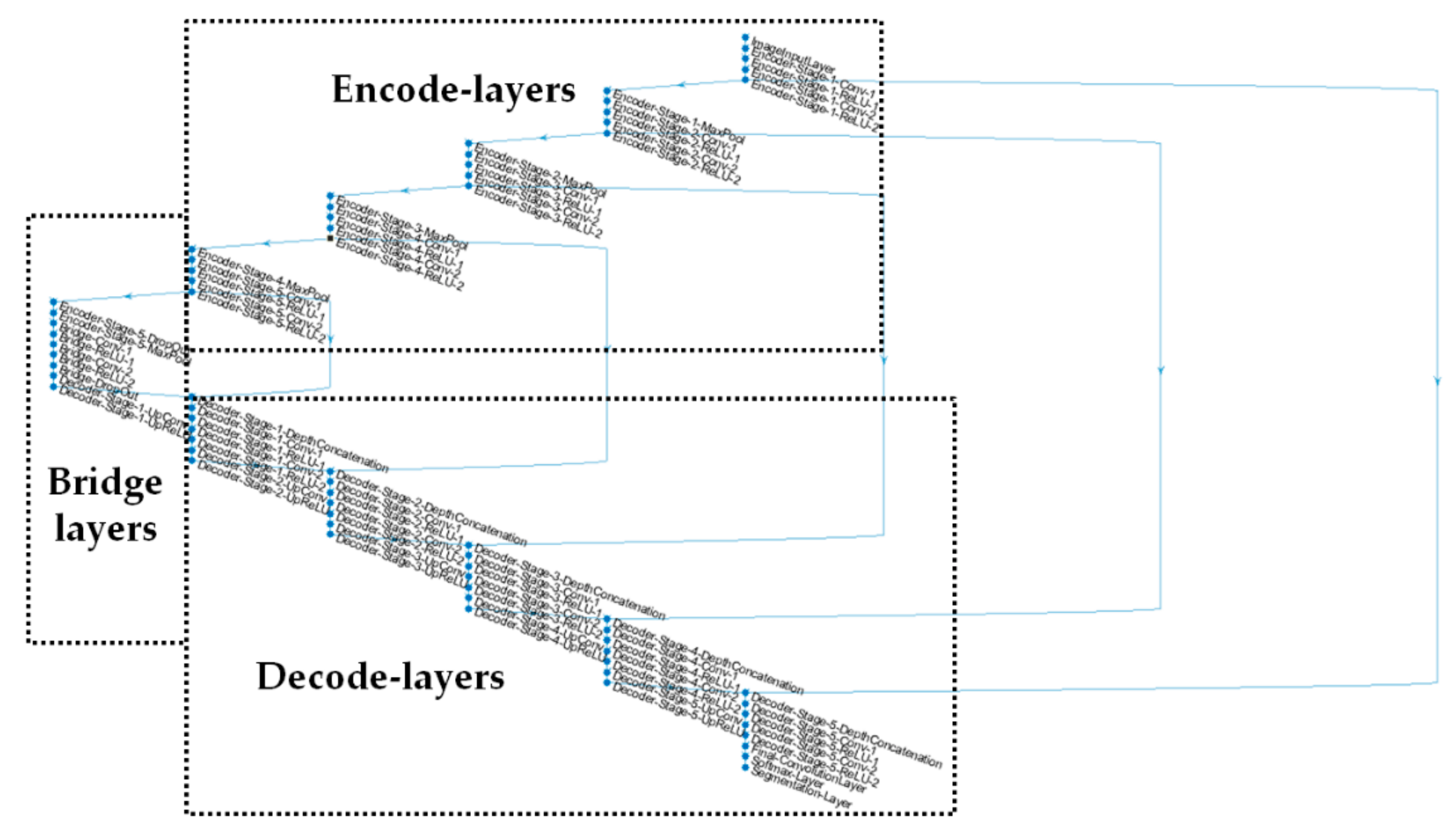
    Figure 1. (a) Details of stepper motor module; (b) acquisition environment.
    Figure 1. (a) Details of stepper motor module; (b) acquisition environment.
    Applsci 10 00139 g001
    Figure 2. Apparatus of the proposed inspection system. (a) Bionic ear; (b) Acquisition computer.
    Figure 2. Apparatus of the proposed inspection system. (a) Bionic ear; (b) Acquisition computer.
    Applsci 10 00139 g002
    Figure 3. Architecture of our proposed anthropomorphic auditory pattern recognition system. Ventral and dorsal flow parts take the original time-frequency spectrum and time spectrum as input. CNN, convolutional neural network.
    Figure 3. Architecture of our proposed anthropomorphic auditory pattern recognition system. Ventral and dorsal flow parts take the original time-frequency spectrum and time spectrum as input. CNN, convolutional neural network.
    Applsci 10 00139 g003
    Figure 4. Structure diagram of hopping feature extraction network.
    Figure 4. Structure diagram of hopping feature extraction network.
    Applsci 10 00139 g004
    Figure 5. (a,b,e,f) Input spectrum graphs; (c,g) optical flow characteristic graphs; (d,h) feature graphs extracted by HoppingNet.
    Figure 5. (a,b,e,f) Input spectrum graphs; (c,g) optical flow characteristic graphs; (d,h) feature graphs extracted by HoppingNet.
    Applsci 10 00139 g005aApplsci 10 00139 g005b
    Figure 6. Schematic diagram of spatial direction convolution; ω = 3 .
    Figure 6. Schematic diagram of spatial direction convolution; ω = 3 .
    Applsci 10 00139 g006
    Figure 7. (a) The workpiece with normal sound and its characteristic pictures. The first two are inner gear, the second one is outer gear, and both with pure time-frequency spectrum. (b) The workpiece with low sound, in the low frequency band there is a noise that is not perceptible to the human. (c) The workpiece with collision sound. The main features are covered by the collision features. (d) The workpiece containing noise sound.
    Figure 7. (a) The workpiece with normal sound and its characteristic pictures. The first two are inner gear, the second one is outer gear, and both with pure time-frequency spectrum. (b) The workpiece with low sound, in the low frequency band there is a noise that is not perceptible to the human. (c) The workpiece with collision sound. The main features are covered by the collision features. (d) The workpiece containing noise sound.
    Applsci 10 00139 g007aApplsci 10 00139 g007b
    Figure 8. (ac) Lowering process; (d) interfering collision process in the rising process; (eg) lifting process; (h) interfering collision process in the lowering process.
    Figure 8. (ac) Lowering process; (d) interfering collision process in the rising process; (eg) lifting process; (h) interfering collision process in the lowering process.
    Applsci 10 00139 g008
    Figure 9. (af) Original image samples; (gi) main characteristics of the spectrum in the three states, six in input graphs, and three hopping feature maps.
    Figure 9. (af) Original image samples; (gi) main characteristics of the spectrum in the three states, six in input graphs, and three hopping feature maps.
    Applsci 10 00139 g009
    Figure 10. (a) Time-frequency spectrum; (b) the main energy distribution rule.
    Figure 10. (a) Time-frequency spectrum; (b) the main energy distribution rule.
    Applsci 10 00139 g010
    Figure 11. Confusion matrix. NS, normal sound; LS, low sound; N, noise; CS, collision sound.
    Figure 11. Confusion matrix. NS, normal sound; LS, low sound; N, noise; CS, collision sound.
    Applsci 10 00139 g011
    Table 1. General structure HoppingNet. * = information extraction and weight concatenation at this layer. Pixel-Pr = prediction at the pixel level. [128, 2048] = There are many repeated blocks in the encode layer and decode layer. We express the number of convolutional layer channels at the same position in the block by the brackets of the double or half relation.
    Table 1. General structure HoppingNet. * = information extraction and weight concatenation at this layer. Pixel-Pr = prediction at the pixel level. [128, 2048] = There are many repeated blocks in the encode layer and decode layer. We express the number of convolutional layer channels at the same position in the block by the brackets of the double or half relation.
    Layers (Kernel Size, Stride)StepTypeInputOutput
    ImageInputLayerEncode_Block_1 364
    Conv_ Relu_Encoder_1 (3 × 3,1)Encode_Block_1Pad (same)6464
    *Conv_ Relu_Encoder_2 (3 × 3,1)Encode_Block_1Pad (same)6464
    Max_PoolingEncode_Block_ (2–5)Pad (0,0,0,0)6464
    Conv_ Relu_Encoder_1 (3 × 3,1)Encode_Block_ (2–5)Pad (same)64[128,2048]
    *Conv_ Relu_Encoder_2 (3 × 3,1)Encode_Block_ (2–5)Pad (same)[128,2048][128,2048]
    Drop_OutBridge_Block50%[128,2048][128,2048]
    Max_PoolingBridge_BlockPad (0,0,0,0)20484096
    Conv_ Relu_Bridge _1 (3 × 3,1)Bridge_BlockPad (same)40964096
    Conv_ Relu_Bridge _2 (3 × 3,1)Bridge_BlockPad (same)40964096
    Drop_OutBridge_Block50%40964096
    UpConv_ UpRelu_ Bridge_1 (2 × 2,2)Bridge_BlockCrop (0,0)40962048
    *Depth_ Concatenation_ Decode _1Decode_Block_ (1–4) 4096[4096,512]
    Conv_ Relu_ Decode _1 (3 × 3,1)Decode_Block_ (1–4)Pad (same)[2048,128][2048,64]
    Conv_ Relu_ Decode _2 (3 × 3,1)Decode_Block_ (1–4)Pad (same)[2048,64][2048,64]
    UpConv_ UpRelu_ Decode_1 (2 × 2,2)Decode_Block_ (1–4)Crop (0,0)[2048,64][2048,64]
    *Depth_ Concatenation_ Decode _1Decode_Block_5 128128
    Conv_ Relu_ Decode _1 (3 × 3,1)Decode_Block_5Pad (same)12864
    Conv_ Relu_ Decode _2 (3 × 3,1)Decode_Block_5Pad (same)641
    Final_Conv_Seg_OutDecode_Block_5 1Pixel-Pr
    Table 2. General structure of temporal CNN. Pad = padding. BN = batch normalization.
    Table 2. General structure of temporal CNN. Pad = padding. BN = batch normalization.
    Layers (Kernel Size, Stride)TypeInputOutput
    ImageInputLayer 1515
    Conv_ Relu_BN_1 (7 × 7,2)Pad (same)15128
    Average_Pooling (2 × 2)Pad (0,0,0,0)128128
    Conv_ Relu_2 (5 × 5,2)Pad (same)128512
    Average_Pooling (2 × 2)Pad (0,0,0,0)512512
    Conv_ Relu_ 3 (3 × 3,1)Pad (same)5121024
    Conv_ Relu_ 4 (3 × 3,1)Pad (same)5122048
    Conv_ Relu_ 5 (3 × 3,1)Pad (same)20484096
    Average_Pooling (2 × 2)Pad (0,0,0,0)40964096
    Fully_Connection_Drop_Out50%40962048
    Fully_Connection_Drop_Out50%2048512
    Fully_Connection 5124
    Table 3. Contribution matrix of principal component analysis of the eigen quantities of 14 dimensions. When the dimensions are reduced to five to reconstruct the eigen signals, the loss quantity shows an inflection point.
    Table 3. Contribution matrix of principal component analysis of the eigen quantities of 14 dimensions. When the dimensions are reduced to five to reconstruct the eigen signals, the loss quantity shows an inflection point.
    ComponentInitial Eigenvalues
    Total% of VarianceCumulative %
    19,29366.37666.376
    22.14015.28381.658
    30.9586.84388.501
    40.4753.39391.894
    50.4233.02094.913
    60.3292.35197.264
    70.2451.74799.011
    80.0510.36599.376
    90.0480.34299.718
    100.0230.16599.883
    110.0100.07099.954
    120.0050.03799.991
    130.0010.00899.999
    140.0000.001100.000
    ComponentExtraction Sums of Squared Loadings
    Total% of VarianceCumulative %
    19.29366.37666.376
    22.14015.28381.658
    30.9586.84388.501
    40.4753.39391.894
    50.4233.02094.913
    Table 4. (a) Different accuracy of model based on different dropout ratio, fusion ratio, and method of pre-training; (b) different configuration of input data; (c) correct detection of each network.
    Table 4. (a) Different accuracy of model based on different dropout ratio, fusion ratio, and method of pre-training; (b) different configuration of input data; (c) correct detection of each network.
    (a) Training Setting
    SettingAccuracy (%)
    Dropout ratio (0.9)91.7
    Dropout ratio (0.7)93.1
    Dropout ratio (0.5)93.6
    Sum fusion ratio (1:1)87.6
    Sum fusion ratio (1:2)91.6
    Sum fusion ratio (1:1.5)93.8
    Pre-trained94.2
    Pre-trained + finetuning96.1
    (b) Input Configuration
    ConfigurationAccuracy (%)
    Spectrogram stacking (S = 30)87.5
    Spectrogram stacking (S = 20)88.4
    Spectrogram stacking (S = 15)91.2
    Cropped-jittering92.5
    Calsse-weight94.2
    (c) Comparison of Models
    MethodAccuracy (%)
    Improved dense trajectories78.2
    Temporal CNN78.3
    Spatial CNN81.2
    Two-stream (SVM fusion)95.8
    Two-stream (average fusion)93.6
    Ours (1:1.5 sum)96.1
    Table 5. According to the data of this task, several mainstream models are tested.
    Table 5. According to the data of this task, several mainstream models are tested.
    MethodAccuracy (%)
    VGG-19 (time-frequency spectrum)78.2
    Densenet201 (time-frequency spectrum)84.5
    Double-branch learning [26]88.4
    Spatiotemporal convolutional—neural [28] (time spectrum)93.8
    Ours (1:1.5 sum)96.1

    Share and Cite

    MDPI and ACS Style

    Fang, X.; Fang, H.; Feng, Z.; Wang, J.; Zhou, L. Artificial Auditory Perception Pattern Recognition System Based on Spatiotemporal Convolutional Neural Network. Appl. Sci. 2020, 10, 139. https://doi.org/10.3390/app10010139

    AMA Style

    Fang X, Fang H, Feng Z, Wang J, Zhou L. Artificial Auditory Perception Pattern Recognition System Based on Spatiotemporal Convolutional Neural Network. Applied Sciences. 2020; 10(1):139. https://doi.org/10.3390/app10010139

    Chicago/Turabian Style

    Fang, Xia, Han Fang, Zhan Feng, Jie Wang, and Libin Zhou. 2020. "Artificial Auditory Perception Pattern Recognition System Based on Spatiotemporal Convolutional Neural Network" Applied Sciences 10, no. 1: 139. https://doi.org/10.3390/app10010139

    Note that from the first issue of 2016, this journal uses article numbers instead of page numbers. See further details here.

    Article Metrics

    Back to TopTop