Article

Saltwater Intrusion in the Upper Tagus Estuary during Droughts

Laboratório Nacional de Engenharia Civil, Avenida do Brasil, 101, 1700-066 Lisbon, Portugal
*
Author to whom correspondence should be addressed.
Geosciences 2019, 9(9), 400; https://doi.org/10.3390/geosciences9090400
Submission received: 26 July 2019 / Revised: 29 August 2019 / Accepted: 11 September 2019 / Published: 14 September 2019

Abstract

:
Droughts reduce freshwater availability and have negative environmental, economic, and social impacts. In estuaries, the dynamics between the saltwater and the freshwater can be affected during droughts, which can impact several natural resources and economic sectors negatively. The Tagus estuary is one of the largest estuaries in Europe and supports diverse uses and activities that can be affected by the saltwater intrusion (e.g., agriculture). This study assesses the saltwater intrusion in the upper reaches of the Tagus estuary using a process-based model to explore different scenarios of freshwater discharge and sea level rise. For the river discharge and mean sea level rise scenarios analyzed, salinity can reach concentrations that are inadequate for irrigation when the mean Tagus river discharge is similar or lower than the ones observed during recent droughts (22–44 m3/s). Lower river discharges aggravate the consequences. Results also show that the salinity increases with the duration of the droughts. In contrast, the impact of a moderate sea level rise on salinity intrusion is modest when compared with the impact of low river discharges. These findings contribute to support the management of the agricultural activities in the upper Tagus estuary and the water resources in the Tagus river basin.

1. Introduction

Extreme weather events, such as droughts, can have negative environmental, economic, and social impacts. Droughts reduce freshwater availability and affect many economic sectors, such as public water supply, agriculture, energy production and tourism [1,2,3]. The decrease in water quantity and quality during droughts can also have negative impacts on the ecosystems, by potentiating harmful algal blooms [4] and reducing the primary productivity [5] or the benthic fauna [6], for example. About 20% of Europe has high to very high vulnerability to droughts [3]. Moreover, the severity of droughts can increase in the future, as global warming can increase their frequency and intensity [7,8].
Estuaries are particularly susceptible to extreme weather events and several estuaries around the world are subject to periodic droughts (e.g., [5,6,9]). In estuarine areas, the dynamics between the saltwater and the freshwater is of major relevance, because it affects residual velocities, residence times, and water quality. This dynamics can be affected during droughts. Since tides and the freshwater discharge are the main drivers of this dynamics, during low river discharge periods the saltwater can propagate further upstream. Salinity is, thus, one of the major stressors associated with droughts in estuaries [10] and the estuarine response to changes in salinity can occur at different time scales [11]. Changes in the salinity dynamics can affect several resources and economic sectors, such as public health, the fishing industry and the aquifers found near estuaries [11]. The impacts of droughts in estuaries can be aggravated by water diversions along the basin [9], but the appropriate management of reservoirs during a drought can help mitigate critical estuarine freshwater inflow problems [10].
The estuarine dynamics and its susceptibility to droughts can be assessed using numerical models, contributing to the definition of management measures. Models have been widely used to study the salinity dynamics in estuaries and their response to climatic forcings (e.g., [12,13,14,15]).
This study uses a numerical model to assess the saltwater intrusion in the Tagus estuary (Portugal, Figure 1). The Tagus estuary is located in the transnational Tagus River basin (Spain–Portugal). The hydrological regime of the Tagus River is heavily modified by several large dams built in the river and its tributaries. The anthropogenic changes in the Spanish part of basin reduced the daily average flow by about 27% at the Portuguese–Spanish border [16]. Several competing water uses occur along the watershed (hydropower generation, public water supply, and irrigation). Thus, the water resources management in the Tagus river basin is both challenging and a requirement, in particular, to guarantee the water availability downstream. The estuary itself supports diverse uses and activities (e.g., urban, industrial/harbors, agriculture, and shellfish harvesting) and its ecological and natural values are well recognized. The western and northern margins of the estuary are intensively occupied by densely urbanized areas, while productive agricultural areas occupy the eastern side [17]. The combined effect of tides and river flow is the main driver of the salinity intrusion in the Tagus estuary [18]. A reduction of the freshwater discharge entering the Tagus estuary may increase the landward intrusion of saltwater and impact some of the uses and activities in the upper estuary negatively, such as agriculture and public water supply. A particular example is the Lezíria Grande de Vila Franca de Xira Public Irrigation Perimeter (Lezíria Grande PIP, Figure 1). The Lezíria Grande PIP is located in low elevation terrains and is surrounded by protection dikes. The main water supply of this irrigated area is located close to the limit of the salinity intrusion in the Tagus estuary. During the most recent droughts (2005 and 2012), the agricultural activities in this area were affected and several emergency measures were undertaken to minimize the negative impacts of the droughts [19]. Moreover, sea level rise can aggravate the salinity intrusion (e.g., [20]).
A process-based model was previously implemented, calibrated and validated in the Tagus estuary [18] using the community model SCHISM [21]. That model is used herein to explore different scenarios of freshwater discharge and sea level rise and assess the saltwater intrusion in the upper reaches of the estuary. Some studies addressed the salinity dynamics in the Tagus estuary, but the present knowledge of the salinity dynamics in the upper estuary remains limited. Most of the recent studies focused in the middle and downstream area of the estuary [18,22,23] and past studies of the upper estuary [24] did not take advantage of cross-scale simulation models, such as the one used herein. The previous implementation of SCHISM [18] is thus extended and applied herein to provide a better understanding of the salinity dynamics and its drivers in the upper Tagus estuary, in particular during droughts. This knowledge can support the definition of management and adaptation measures during droughts and help the end-users coping with future changes.
The paper is organized in three sections besides the present introduction. Section 2 describes the methodology used, including the setup of the numerical model and the scenarios simulated. The results and discussion are presented in Section 3. Section 4 summarizes the main conclusions.

2. Materials and Methods

2.1. Study Area

The Tagus estuary has an area of about 320 km2 and connects to the Atlantic Ocean through a deep, long and narrow inlet (Figure 1). The mid estuary is characterized by a shallow inner basin with extensive tidal flats and marshes that narrows about 40 km upstream of the inlet (Figure 1). The intertidal area represents about 43% of the total estuarine surface [25].
Tides are the main driver of the circulation in the Tagus estuary. Tides are semi-diurnal with tidal ranges at the coast varying between 0.55 m and 3.86 m [26]. This range is significantly amplified within the estuary due to resonance effects [27,28].
Other drivers, such as river flow, wind, atmospheric pressure, and surface waves, may also influence the circulation within the estuary during storms [29]. Downstream, the water levels are mainly controlled by tides and storm surges. In the upper estuary (farther than 40 km upstream of the mouth), river discharge may significantly influence water levels. The main affluent of the Tagus estuary is the Tagus River, with a mean river discharge of 336 m3/s [30]. Two other rivers, the Sorraia River (about 5% of the Tagus river discharge, [31]) and the Trancão River, also contribute to the freshwater inflow to the estuary. The estuary is often considered well-mixed, but stratification can occur for high river flows and low tidal ranges [18,32].

2.2. Model Application

2.2.1. Model Setup

The dynamics of the Tagus estuary was simulated with the community model SCHISM [21] in three-dimensional baroclinic mode. This community model evolved from SELFE [33] and aims at the cross-scale simulation of surface water processes from the river to the ocean [34]. SCHISM is fully parallelized. The model uses semi-implicit finite element and finite volume methods, combined with Eulerian–Lagrangian methods, to solve the shallow water equations. SCHISM is based on unstructured grids in the horizontal dimension and uses hybrid SZ coordinates or LSC2 (Localized Sigma Coordinates with Shaved Cell [35]) in the vertical dimension. SCHISM and its predecessor SELFE have been extensively used to simulate the three-dimensional estuarine circulation and salinity gradients and, thus, the processes relevant to the present application (e.g., [13,34,36,37]). The use of unstructured grids is also advantageous in the present application, in particular the in upstream area, as it allows a better representation of the marginal structures (e.g., protection dikes of the Lezíria Grande PIP, Figure 1).
To accurately represent all the relevant physical processes, the model domain includes the whole estuary, from the river to the ocean (Figure 2). The horizontal grid has about 83,000 nodes and a typical resolution of 15–25 m in the inner channels and 1–2 km in the coastal boundary. The vertical domain is discretized with a hybrid grid with 39 levels (30 S levels in the upper 100 m, and 9 Z levels between 100 m and the maximum depth). The numerical model is forced by: Tides at the ocean boundary, river flows at the riverine boundaries (Tagus and Sorraia) and atmospheric data at the surface. The time step is set to 30 s. Further details regarding the model setup can be found in [18]. The model has been previously calibrated and extensively validated in the Tagus estuary and the results showed its ability to represent the circulation and salinity patterns [18]. In Vila Franca de Xira (the station located farther upstream where data were available; see Figure 1 for location) salinity errors were about 2 psu and the model skill was about 0.9 for a period of low to average river flows [18].

2.2.2. Model Validation for Droughts and Sensitivity Analyses

The previous validation of the salinity model was done for low to average and high river flow conditions [18] and did not extend until the limit of the upper estuary, which is the focus herein. Fortunately, data at the Conchoso station for drought conditions became available for July 2017, after the previous validation was carried out [18]. Thus, the validation of the salinity model for drought conditions was extended for July 2017.
Preliminary simulations were performed for July 2005 (period during which one of the worst recent droughts occurred) and a sensitivity analysis to the river flow was done. For this period, the river flow was estimated as 22 m3/s based on [38]. These simulations showed that the model results are very sensitive to the river flow, in particular in the upper estuary (Figure 3). Thus, the accuracy of the model requires adequate estimates of the river flow.
River flow data are usually available at the Almourol station (see Figure 1 for location). However, this dataset has failures and alternative datasets must be explored. Therefore, the accuracy of the river flow data was assessed. This assessment compared two datasets: i) the river flow data from the Almourol station (Figure 1), upstream of the estuary, and ii) the sum of the outflow from the two dams that drain into the lower Tagus River—Castelo de Bode, located in the Zêzere, an affluent to the Tagus River and Belver, the dam in the Tagus River closest to the estuary (Figure 1). The comparison was restricted to the last decade (hydrological years 2008–2009 to 2016–2017). All these data are available at the Portuguese water resources information portal (http://snirh.pt).
Since there are no significant inflows or water abstractions between the two dams and the Almourol station, the time series were expected to be similar. However, the comparison between the two time series reveals significant differences (Figure 4). The mean river flow is significantly smaller for the Almourol data than for the dams: 219 and 261 m3/s, respectively, considering only the days with data available for both time series. The discrepancy between the two time series was estimated as the difference between the Almourol and the dams data, scaled by the average of the two time series for each day. This discrepancy varies between −150% and 200%, and the mean of the absolute value of this discrepancy is 42%. Furthermore, the discrepancy is particularly significant for small river flows (Figure 5), when salinity intrusion is highest. The discrepancy can be both positive and negative, which excludes a systematic error associated with a source or abstraction of water between Almourol and the dams. The error could be partly due to an inadequate extrapolation of the relationship between the river flow and the water level measurements at Almourol, which would explain the concentration of points along a well-defined function in Figure 5. However, the spread around that function also suggests that there are other sources of errors. Hence, the accuracy of the river flow data is questionable.
Given the uncertainty on the river flow data, the July 2017 simulations were forced by two alternative input flows at the upstream boundary: data from Almourol and the sum of the outflows from the two dams. This assessment aimed to evaluate the influence of the alternative river flows on the model results.
An additional potential source of model errors is the model bathymetry upstream of Vila Franca de Xira. Upstream of that point, only cross-sectional data of the river and estuary are available, with a longitudinal spacing of over 2 km. In previous model applications, these data have been used to generate a very simple model bathymetry using rectangular cross-sections with varying width and depth. Because this simplification can potentially affect the proper reproduction of tidal propagation and salinity intrusion, a sophisticated approach to transform the cross-sectional data into a 2D bathymetry was developed, loosely based on [39] (see Appendix A). This new approach was used to represent the bathymetry upstream of Vila Franca de Xira. To evaluate the influence of the bathymetry in the model results, the 2017 simulation was repeated using the new bathymetry.

2.2.3. Scenarios Setup

The simulated scenarios were selected in close collaboration with the end-users during several workshops (e.g., [40]) and specific meetings. Five scenarios were considered for the Tagus river discharge. These scenarios were established for July. The summer season is the most critical during droughts and during past events the most severe situations for agricultural activities begun around this month. The river discharge scenarios were based on historical data, and took into account some of the water uses in the basin (e.g., hydropower generation) and the established agreements between Portugal and Spain regarding the water management in the Tagus River basin. Additionally, a mean sea level rise (SLR) scenario of 0.5 m was also considered at the oceanic boundary. To establish identical and realistic initial conditions for all the scenarios, a simulation was performed for the period between March 15 and June 30. The simulated scenarios were the following:
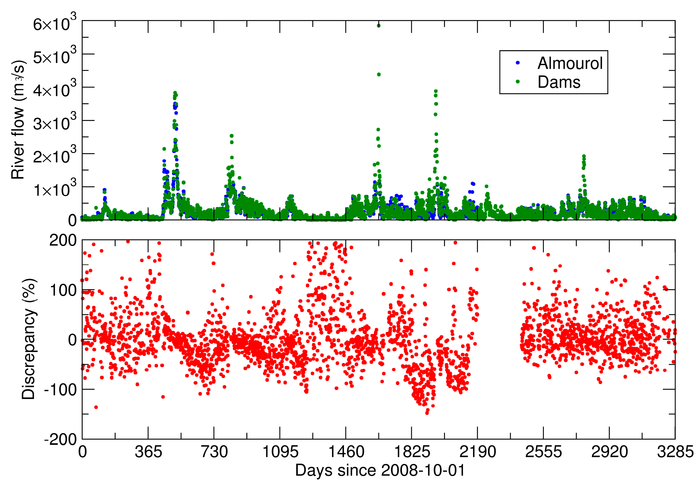
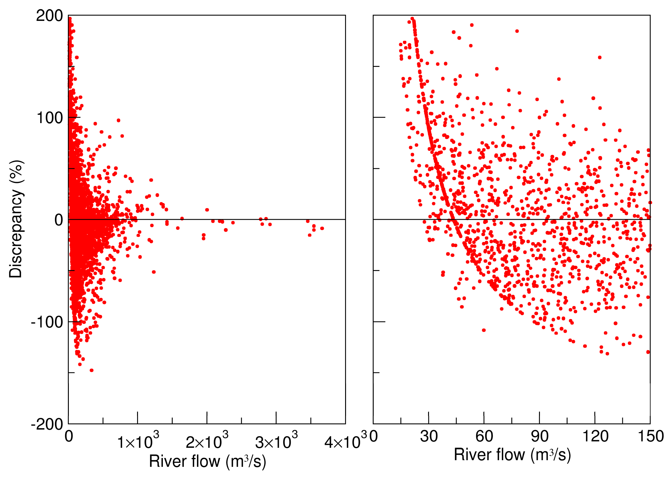
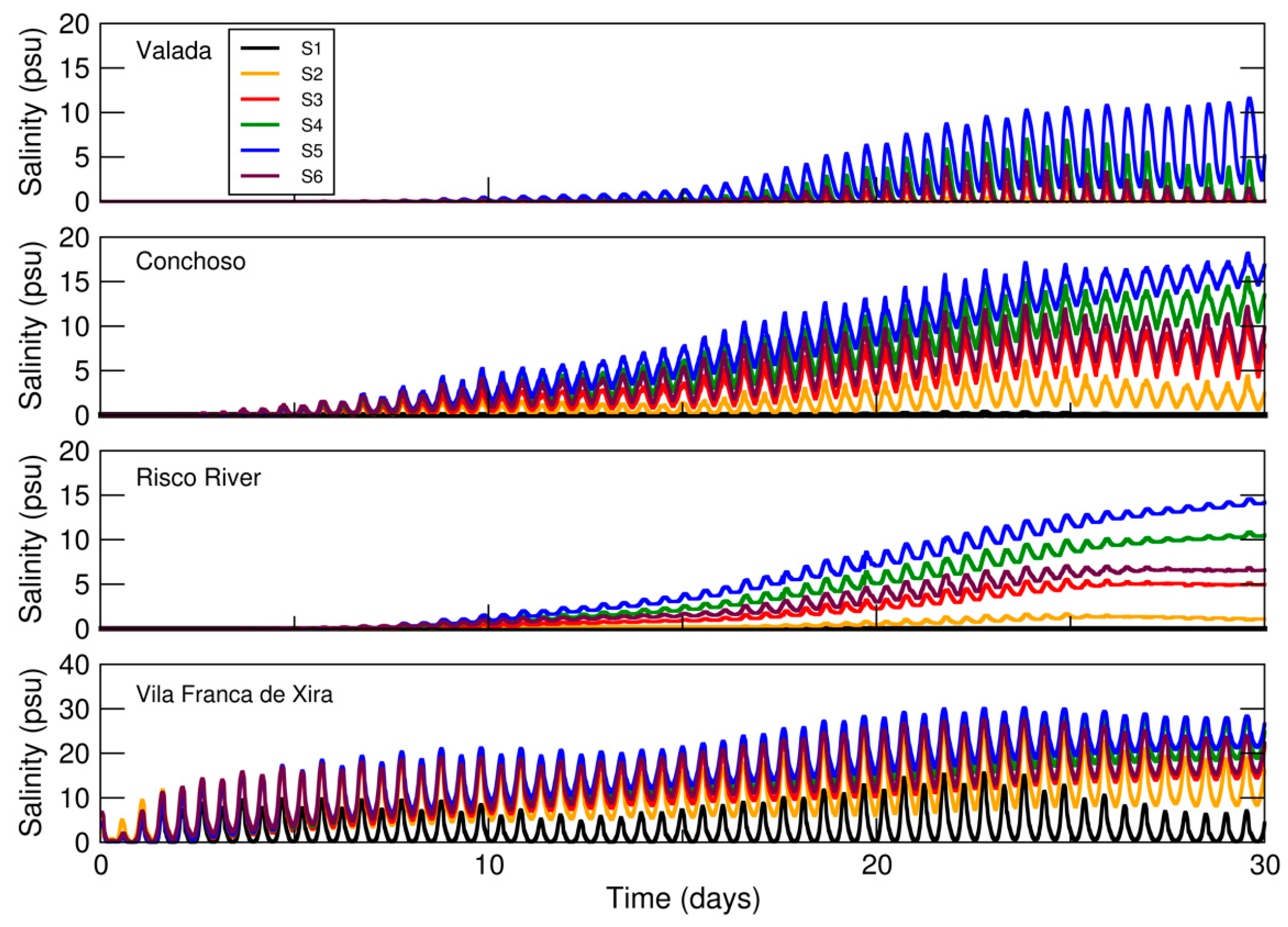
  • Scenario 1, climatological scenario—river flow of 132 m3/s: scenario based on the climatological analysis of the mean daily discharge at the Almourol station (http://snirh.pt) between 1990 and 2017 during July.
  • Scenario 2, recent drought—river flow of 44 m3/s: scenario that represents one of the recent droughts, which occurred in 2012. Water scarcity issues occurred in the Lezíria Grande PIP in 2012 and water with a salinity of about 1.2 psu was used for irrigation, which reduced the production of the crops. The river flow used in this scenario was estimated based on data measured at Almourol (http://snirh.pt).
  • Scenario 3, worst recent drought—river flow of 22 m3/s: scenario that represents one of the worst recent droughts, which occurred in 2005. In 2005, from mid-July onwards, the water supply to the Lezíria Grande PIP was made exclusively from the Risco River. In mid-August, the salinity at the Risco River was 1 psu (comparatively to typical values of 0.3 psu) and a temporary weir was built in the Sorraia River to route the freshwater available in this river. The adverse impacts of the 2005 drought were more severe for the farmers than in 2012: the drought itself was more severe and the farmers were less prepared to deal with these events. Because data at Almourol are unavailable for this period, the river flow was estimated based on [38] using data measured at Matrena and Tramagal (http://snirh.pt).
  • Scenario 4, minimum river flow—river flow of 16.5 m3/s: scenario based on the revised Spanish-Portuguese Albufeira Convention and Additional Protocol (Portuguese Parliament Resolution n. 62/2008, November 14). This river flow represents the minimum mean weekly flow that must be guaranteed between 1 July and 30 September near the upstream boundary of the Tagus estuary (Muge). However, the Convention considers the possibility of an exception during very dry years, and this weekly minimum value is not always achieved [41]. Also, the minimum weekly river flow at the Portuguese / Spanish border can be (and often is) achieved by discharging only a few hours per week [41], to maximize electricity production.
  • Scenario 5, worst-case scenario – river flow of 8 m3/s: this value represents the minimum river flow that guarantees the operation of one of the primary thermoelectric power plants in the Tagus River basin.
  • Scenario 6, sea level rise—sea level rise of 0.5 m and river flow of 22 m3/s: this scenario combines a recent drought with a possible sea level rise for the end of the century [7]. The median values of SLR between 1986–2005 and 2081–2100 depend on the Representative Concentration Pathway (RCP). Typical values vary between about 0.4 m for RCP2.6 and 0.7 m for RCP8.5 [42]. Considering that our starting point already incorporates the SLR until 2017, this scenario can be considered a high-end estimate.
The river flow at the Tagus River boundary was established as described above. In the Sorraia River, the river flow was taken as 5% of the river flow in the Tagus River, based on the ratios between annual averages in the two rivers, following an approach similar to the one used for the calibration and validation of the model [18].
To allow the comparison between the river flow scenarios, the oceanic and atmospheric forcings were similar in all the simulations and aimed to be representative of average conditions.
To set up the tide, the tidal amplitudes at Cascais (near the coastal boundary of the model) were determined between 1991 and 2010 using the tides from the regional model of [43]. For each year, the mean and the standard deviation were computed for the period from April to October, covering the period during which the simulations are performed. The comparison of these values with their global mean and standard deviations indicates that the year 2001 is the most representative of average conditions (Figure S1—Supplementary material).
A similar approach was used to define the atmospheric forcing for the scenarios simulations. Because the atmospheric forcing has little influence on the salinity results [18], a single set of representative atmospheric conditions was used for all simulations. This set of conditions was taken from decadal predictions of the climate evolution for 2018–2024 [44]. This dataset includes 10 realizations. Mean values of air temperature, atmospheric pressure and wind intensity for the summer-spring period (between March and July) were computed for each pair of realization and year between 2018 and 2024. The means were determined at two stations representative of the upper and the lower estuary (Vila Franca de Xira and Cascais, respectively). The realization with means closest to the global mean of the three variables was selected as representative conditions. Results indicate that for both stations the realization 3 for the year 2022 is the most representative of the average conditions (Figure S2—Supplementary material).

3. Results and Discussion

3.1. Sensitivity to the River Flow and Bathymetry

Results indicate that for both river flows datasets the model correctly reproduces the phase of the signal associated with the tide, but tends to overestimate the maximum salinity (Figure 6). Root Mean Square Error (RMSE) and Mean Absolute Error (MAE) are 0.4 psu and 0.3 psu, respectively, with the river flow data from Almourol. For this simulation, the maximum difference between the data and the model results at the peak salinity is about 2 psu. For the simulation using the data from Castelo de Bode and Belver dams, RMSE and MAE are, respectively, 2.8 psu and 2.2 psu and the maximum difference at the peak salinity is about 8 psu. The river flow data from Almourol (the closest station to the model boundary) provides, thus, the best model results. Results suggest that the use of the data from the Castelo de Bode and Belver dams to establish the river flow for the simulations is not a feasible alternative to the Almourol data. Results also show that the discrepancy between the two simulations with the different river flows largely exceeds the error between the best model result and the data. This behavior suggests that the uncertainty in the river flow data dominates the errors in the model results for the salinity.
Regarding the upstream bathymetry, results show that the differences between the two simulations are minor (Figure 7), with mean absolute difference smaller than 0.1 psu (range 0–0.7 psu). These results, together with the results discussed previously for the two alternative river flows, show that the river flow is the main source of uncertainty in the salinity model results in the upper Tagus estuary. Accurate estimations of the Tagus river flow are thus fundamental to ensure good model results.

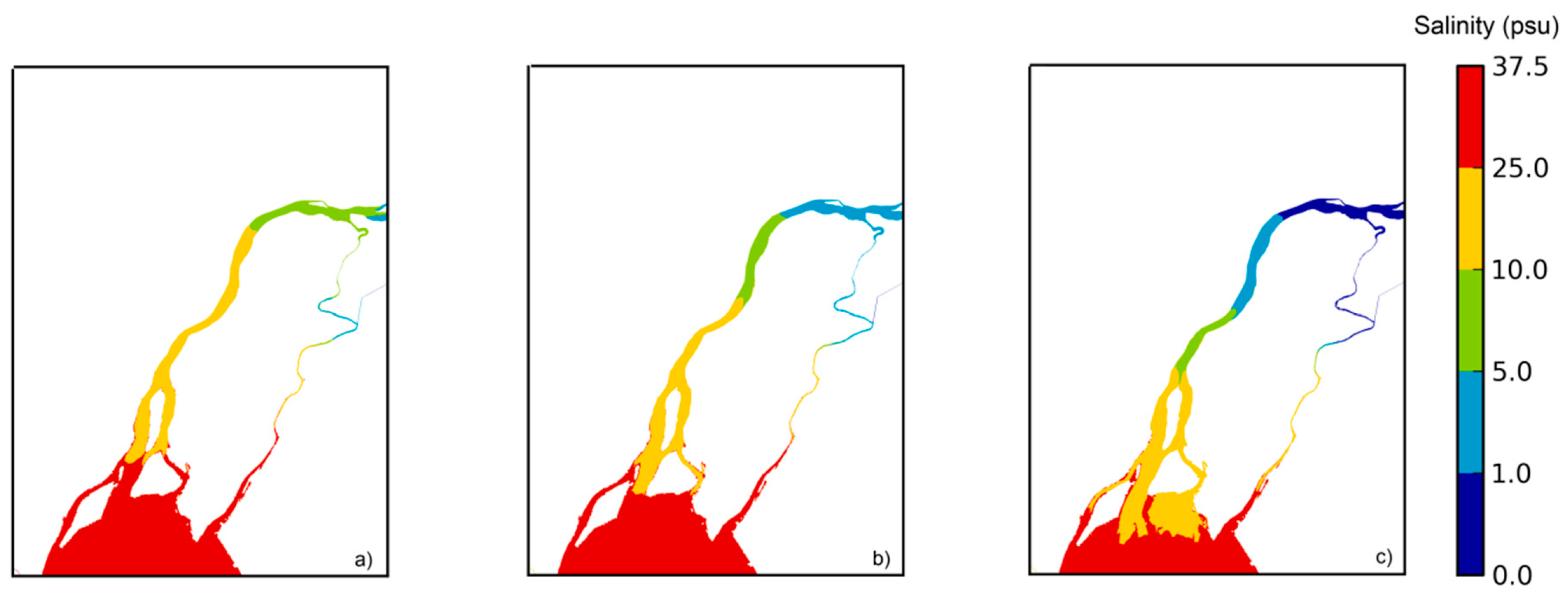
3.2. Saltwater Intrusion Relative to River Discharge and Slr Scenarios

Time series of salinity were extracted from the model at four stations located in the upper Tagus estuary (Figure 1): i) Vila Franca de Xira, ii) Conchoso, where the main water abstraction for irrigation is located, iii) Risco River, a possible alternative water abstraction for irrigation and iv) Valada, where a water abstraction for public water supply is located. The analysis of these time series (Figure 8) and the corresponding statistics (Figure 9) provide detailed insight into the saltwater intrusion in the upper Tagus estuary under drought conditions.
For climatological conditions (scenario 1—mean Tagus river flow of 132 m3/s), salinity does not reach the Conchoso, Risco River and Valada stations. This behavior is consistent with the empirical knowledge of the farmers and provides confidence in the model results.
For the recent drought (scenario 2—estimated mean Tagus river flow of 44 m3/s), salinity remains low at Valada and Risco River stations. At the Conchoso station, an increasing trend is observed and at high tide salinity can reach values that exceed the limit acceptable for irrigation (salinity less than 1 psu) by the end of the simulation. The estimated salinity is, however, lower than in scenario 3.
For the worst recent drought (scenario 3—estimated mean Tagus river flow of 22 m3/s), salinity remains relatively low at Conchoso for the first 15 days of simulation, with values ranging from 0 psu at low tide to about 2.5 psu at high tide. After this period, salinity increases and varies between about 5 psu and 10 psu at this station. These values largely exceed the limit acceptable for irrigation. The exceedance of the salinity threshold acceptable for irrigation is consistent with testimonies from the farmers in the region regarding the 2005 and 2012 droughts [45]. In particular, the relative differences between the estimated peak salinity for these two simulations are of the same order of magnitude of those observed by the farmers in 2005 and 2012 (ABLGVFX, personal communication), providing further confidence in the model. At the Risco River, the salinity exhibits minimal tidal oscillations and the maximum salinity reaches about 5 psu for scenario 3. Salinity remains lower than 1 psu for the first 15 days of simulation at this station. For the same scenario, the maximum salinity at Valada reaches about 5 psu. This value is probably too high to use this water for public water supply. However, salinity only appears to be a problem at Valada for this scenario during high spring tides. During neap tides, the salinity remains very low, within acceptable limits for public water supply.
For the minimum river flow agreed upon by the Portuguese and Spanish authorities for the July–September period (scenario 4—mean Tagus river flow of 16 m3/s), salinity also presents an increasing trend along the simulated period. At Conchoso, the minimum salinity exceeds 5 psu after 10 days of simulation and the maximum salinity reaches about 15 psu. These concentrations make the water inadequate for irrigation at Conchoso. At Risco River, for the last 15 days of simulation, the salinity is about the double of the salinity estimated for scenario 3. For scenario 4, salinity is also higher at Valada, with maximum values reaching about 7 psu and preventing the water abstraction during high tide. During low tide, salinity remains close to 0 psu at Valada. Further reducing the river flow, as simulated in scenario 5 (mean Tagus river flow of 8 m3/s), increases the salinity at all the stations and aggravates the consequences for both irrigation and water supply. Although different scenarios were analyzed, the results of the present study present similar trends to those obtained by [24].
For the mean sea level rise scenario (scenario 6—SLR of 0.5 m and mean Tagus river flow of 22 m3/s), salinity is only slightly higher than the values observed for scenario 3 with the same river flow. Between these two scenarios, salinity differences are typically less than 1 psu and smaller when compared with the differences between the river flow scenarios. These results suggest that in short to medium term, the freshwater inflow is the main driver controlling the salinity in the upper reaches of the estuary. Considering the small sensitivity of salinity intrusion in the Tagus to SLR and that the SLR scenario analyzed can be considered a high-end estimate, no other scenarios of SLR were investigated.
In general, results show that the tidally-averaged salinities display a rising trend even after one month of simulations with constant river flows. This behavior shows that salinity intrusion in the upper estuary depends not only on the river flow alone but also on the duration of the droughts.

3.3. Water Availability for Irrigation

The tidal signal present in the salinity time series suggests that, under drought conditions, water should only be abstracted from the river at low tide to provide fresher water. A plot of the salinity versus water elevation (Figure 10) confirms that the highest salinities occur close to high tide. The exception is Risco River where the salinity exhibits minimal variations with the tide. At this station, salinity is similar to the minima observed at Conchoso at each tidal cycle (Figure 8). The small oscillations suggest that the same water mass sloshes back and forth, with small exchanges with the Tagus River. This water mass is relatively small, thus creating an alternative source for water irrigation in this area would not solve the water shortage problem during a drought. Indeed, estimating the volume of the Risco River at 1–4 × 10⁶ m3 and considering a pumping rate of 0.7 × 10⁶ m3/day, this alternative pumping station would only provide adequate water for less than a week.
To assess the water availability for irrigation, the percentage of time per week during which the salinity of the abstracted water is adequate for irrigation was calculated for each river discharge scenario at Conchoso (Figure 11). Estimates were made considering the salinity threshold of 1 psu as acceptable for irrigation. Taking into account the maximum error in the model peak results discussed in Section 3.1, error bars are also presented for the salinity limit of 3 psu. Results show that salinity is always lower than 1 at Conchoso for scenario 1. For scenario S2, results suggest that there is always some water available for irrigation. For scenario 3, water is adequate for irrigation about 75%–100% of the time in the first two weeks, while for scenario 4 this occurs only in the first week. For the river discharge scenarios 3–5 the water is inadequate for irrigation by the fourth week. It should be noted that in the present simulations the uptake of water for irrigation was not considered in the model, which could contribute to increase the salinity and should be further explored.
These findings can support the management of the agricultural activities in the upper Tagus estuary and the adoption of adaptation measures during droughts. As mentioned above, during the 2005 drought, salinity reached concentrations that were inadequate for irrigation at both the Tagus and the Risco rivers and a temporary weir was built in the Sorraia River to route the freshwater available in this river. At that time, the farmers were not yet prepared to deal with the droughts and the losses in the crops were significant. The timely information about the river discharge and the insights about its influence on the salinity provided herein can support the timely adoption of adaptation measures by the farmers and reduce some of the negative consequences during droughts.
The results obtained herein can support the management of the water resources in the region. They show that the water management must also take into account the economic and ecological impacts downstream and provide insight about the releases of water from the dams. In the established scenarios the river discharge was considered constant during one-month. Variable river discharges should be explored in future research. Considering the uncertainty on the river discharge data available for the Tagus River, accurate river discharge data are also fundamental to appropriately support decision-making in the water resources management in this region.

4. Conclusions

A numerical model was used to assess the saltwater intrusion in the upper Tagus estuary for several scenarios of freshwater discharge and mean sea level rise.
The numerical assessment of the salinity dynamics indicates that the river discharge is the main driver of the salinity in the upper Tagus estuary. For the analyzed river discharge and mean sea level rise scenarios, salinity reaches concentrations that are inadequate for irrigation during some periods when the mean Tagus river discharge is similar or lower than the ones observed during recent droughts (22–44 m3/s). Lower river discharges aggravate the consequences. The duration of the droughts also increases the salinity in the upper Tagus estuary.
The results achieved can contribute to support the management of the water resources in the Tagus river basin and the agricultural activities in the upper Tagus estuary. In particular, they provide insight into the releases of water from dams and information that can support the farmers to adopt timely adaptation measures during low river discharge periods. Accurate estimates of the Tagus river flow are fundamental to support the adequate management of the water resources in the region.

Supplementary Materials

The following are available online at https://www.mdpi.com/2076-3263/9/9/400/s1, Figure S1: Spring/summer means and standard deviations of the tidal range at Cascais between 1991 and 2010, Figure S2: Yearly and global means of the air temperature, atmospheric pressure and wind intensity at Cascais between 2018 and 2024.

Author Contributions

Conceptualization, M.R., A.B.F., and P.F.; Methodology, M.R. and A.B.F.; Validation, M.R.; Simulations, M.R. and A.B.F.; Investigation and Scenarios Analysis, M.R. and A.B.F.; Writing—Original Draft Preparation, M.R.; Writing—Appendix, A.B.F.; Writing—Review and Editing, M.R., A.B.F., and P.F.

Funding

This research was funded by the European Commission through the H2020 project BINGO (Grant Agreement Number 641739) and by the FCT—Fundação para a Ciência e Tecnologia project UBEST—Understanding the biogeochemical buffering capacity of estuaries relative to climate change and anthropogenic inputs (PTDC/AAG-MAA/6899/2014). This work used resources of the Portuguese National Distributed Computing Infrastructure (INCD) funded by Lisboa2020 Operational Program through the INCD project (LISBOA-01-0145-FEDER-022153).

Acknowledgments

The authors would like to thank Joseph Zhang for making the numerical model SCHISM available. The authors thank the Associação de Beneficiários da Lezíria Grande de Vila Franca de Xira (ABLGVX) for providing information about the Public Irrigation Perimeter and making the Conchoso data available. The authors also thank ABLGVFX and Rui Rodrigues for discussions regarding the river flow scenarios’ definition. The authors thank the three anonymous reviewers.

Conflicts of Interest

The authors declare no conflict of interest.

Appendix A. Extracting a 2D Bathymetry from Cross-Sectional Data

Riverine bathymetries are often measured along cross-sections. Usually, the distance between consecutive cross-sections largely exceeds the spacing between soundings along the same cross-section. As a result, using traditional isotropic interpolation methods to generate digital terrain models (DTMs) can be very inaccurate. The generation of the DTMs is further complicated by river bends, constrictions and islands that occur between cross-sections.
To overcome these difficulties, [39] proposed interpolating the bathymetry first along the cross-section, and then between consecutive cross-sections following the streamlines. This appendix describes a different implementation of a similar approach. Contrary to the original method, which determines the lateral river boundaries based on the cross-sectional data, the method implemented herein defines those boundaries using additional more detailed data (e.g., maps, satellite images, orthophoto maps).
The method proceeds as follows. First, the lines defining the river margins are intersected with the cross-sections containing the bathymetric data. Secondly, each cross-section is divided into a user-defined number of equally-space points (NL), between the two end points determined in the first step. NL represents the number of streamlines that will be used in the procedure. The bathymetry is interpolated at those NL points using linear functions or cubic splines. Thirdly, for each river stretch between two consecutive cross-sections, NL streamlines are generated, equally spaced between the two margins. These streamlines are divided into a user-defined number of cross-sections (NPS), equally spaced between the two consecutive cross-sections where bathymetric data are available. At the intersection between the streamlines and user-defined cross-sections, the bathymetry is interpolated linearly between the two endpoints. Finally, when all the points and their bathymetry are defined, a triangular grid is generated. This grid can then be used to interpolate the bathymetry for the model’s computational grid.
Figure A1 illustrates the application of the method in the upper reaches of the Tagus estuary, where cross-sectional data are available at about 2.5 km intervals. The interpolated bathymetry correctly predicts higher depths at the concave side of the meanders and shallower depths at the convex side. Also, the method is convergent with NL and NPS, and the results are smooth. If the linear interpolator is used, results are also bound between the limits imposed by the data. The downside of this approach is its inability to realistically deal with islands and major changes in cross-section that are not represented by the cross-sectional data. For instance, depths are expected to decrease when the river widens, so that the cross-section is approximately constant. These reductions of depth are not reproduced by the method (see the bathymetry between the two easternmost cross-sections in Figure A1).
Figure A1. Extraction of 2D bathymetries from cross-sectional data in the upper Tagus estuary for (NL,NPS) = (5,10) (a) and (NL,NPS) = (20,50) (b). The blue dots indicate the margins and the 5 sections where cross-sectional data are available.
Geosciences 09 00400 g0a1

References

  1. Wilhite, D.A. Drought as a natural hazard: Concepts and definitions. In Drought: A Global Assessment; Wilhite, D.A., Ed.; Routledge: London, UK, 2000; Volume 1, pp. 3–18. [Google Scholar]
  2. Stahl, K.; Kohn, I.; Blauhut, V.; Urquijo, J.; Stefano, L.D.; Acácio, V.; Dias, S.; Stagge, J.H.; Tallaksen, L.M.; Kampragou, E.; et al. Impacts of European drought events: Insights from an international database of text-based reports. Nat. Hazards Earth Syst. Sci. 2016, 16, 801–819. [Google Scholar] [CrossRef]
  3. Poljanšek, K.; Ferrer, M.M.; De Grove, T.; Clark, I. Science for Disaster Risk Management 2017: Knowing Better and Losing Less; Office of the European Union: Luxembourg, 2017. [Google Scholar]
  4. Lehman, P.W.; Kurobe, T.; Lesmeister, S.; Baxa, D.; Tung, A.; Teh, S.J. Impacts of the 2014 severe drought on the Microcystis bloom in San Francisco Estuary. Harmful Algae 2017, 63, 94–108. [Google Scholar] [CrossRef] [PubMed]
  5. Wetz, M.S.; Hutchinson, E.A.; Lunetta, R.S.; Paerl, H.W.; Taylor, J.C. Severe droughts reduce estuarine primary productivity with cascading effects on higher trophic levels. Limnol. Oceanog. 2011, 56, 627–638. [Google Scholar] [CrossRef]
  6. Dittmann, S.; Baring, R.; Baggalley, S.; Cantin, A.; Earl, J.; Gannon, J.; Keuning, J.; Mayo, A.; Navong, N.; Nelson, M.; et al. Drought and flood effects on macrobenthic communities in the estuary of Australia’s largest river system. Est. Coast. Shelf Sci. 2015, 165, 36–51. [Google Scholar] [CrossRef]
  7. IPCC. Climate Change 2013: The Physical Science Basis. Contribution of Working Group I to the Fifth Assessment Report of the Intergovernmental Panel on Climate Change; Stocker, T.F., Qin, D., Plattner, G.K., Tignor, M., Allen, S.K., Boschung, J., Nauels, A., Xia, Y., Bex, V., Midgley, P.M., Eds.; Cambridge University Press: Cambridge, UK; New York, NY, USA, 2013; p. 1535. [Google Scholar]
  8. Hoegh-Guldberg, O.; Jacob, D.; Taylor, M.; Bindi, M.; Brown, S.; Camilloni, I.; Diedhiou, A.; Djalante, R.; Ebi, K.L.; Engelbrecht, F.; et al. Impacts of 1.5 °C Global Warming on Natural and Human Systems. In Global Warming of 1.5 °C. An IPCC Special Report on the Impacts of Global Warming of 1.5 °C above Pre-Industrial Levels and Related Global Greenhouse Gas Emission Pathways, in the Context of Strengthening the Global Response to the Threat of Climate Change, Sustainable Development, and Efforts to Eradicate Poverty; Masson-Delmotte, V., Zhai, P., Pörtner, H.O., Roberts, D., Skea, J., Shukla, P.R., Pirani, A., Moufouma-Okia, W., Péan, C., Pidcock, R., et al., Eds.; Intergovernmental Panel on Climate Change: Geneva, Switzerland, 2018. [Google Scholar]
  9. Palmer, T.A.; Montagna, P.A. Impacts of droughts and low flows on estuarine water quality and benthic fauna. Hydrobiologia 2015, 753, 111–129. [Google Scholar] [CrossRef]
  10. Gilbert, S.; Lackstrom, K.; Tufford, D. The Impact of Drought on Coastal Ecosystems in the Carolinas; Research Report: CISA-2012-01; Carolinas Integrated Sciences and Assessments: Columbia, SC, USA, 2012; p. 67. [Google Scholar]
  11. Conrads, P.; Darby, L. Development of a coastal drought index using salinity data. Am. Meteorol. Soc. 2017, 98, 753–766. [Google Scholar] [CrossRef]
  12. Xu, J.; Long, W.; Wiggert, J.D.; Lanerolle, L.W.J.; Brown, C.W.; Murtugudde, R.; Hood, R.R. Climate Forcing and Salinity Variability in Chesapeake Bay, USA. Estuaries Coasts 2012, 35, 237–261. [Google Scholar] [CrossRef]
  13. Kärnä, T.; Baptista, A.M. Evaluation of a long-term hindcast simulation for the Columbia River estuary. Ocean Model. 2016, 99, 1–14. [Google Scholar] [CrossRef] [Green Version]
  14. Liu, W.C.; Chan, W.T. Assessment of climate change impacts on water quality in a tidal estuarine system using a three-dimensional model. Water 2016, 8, 60. [Google Scholar] [CrossRef]
  15. Wang, J.; Li, L.; He, Z.; Kalhoro, N.A.; Xu, D. Numerical modelling study of seawater intrusion in Indus River Estuary, Pakistan. Ocean Eng. 2019, 184, 74–84. [Google Scholar] [CrossRef]
  16. Rodrigues, R. Coping with Hydrological Risk in Shared Rivers—The Iberian Peninsula Case. In Proceedings of the 1st Thematic Workshop of the EU Coordination Action RISKBASE, Monitoring and Assessment of River Pollutants, Lisbon, Portugal, 17–18 May 2007. [Google Scholar]
  17. Tavares, A.O.; Santos, P.P.; Freire, P.; Fortunato, A.B.; Rilo, A.; Sá, L. Flooding hazard in the Tagus estuarine area: The challenge of scale in vulnerability assessments. Environ. Sci. Policy 2015, 51, 238–255. [Google Scholar] [CrossRef]
  18. Rodrigues, M.; Fortunato, A.B. Assessment of a three-dimensional baroclinic circulation model of the Tagus estuary. AIMS Environ. Sci. 2017, 4, 763–787. [Google Scholar] [CrossRef]
  19. Freitas, A.; Luis, A.; Fortunato, A.; Villanueva, A.; Martins, B.; Russo, B.; Strehl, C.; Martinez, E.; Alves, E.; Bergsma, E.; et al. Risk Identification: Relevant Hazards, Risk Sources and Factors, Deliverable 4.2; BINGO: Lisbon, Portugal, 2017; p. 138. [Google Scholar]
  20. Liu, W.C.; Liu, H.M. Assessing the Impacts of Sea Level Rise on Salinity Intrusion and Transport Time Scales in a Tidal Estuary, Taiwan. Water 2014, 6, 324–344. [Google Scholar] [CrossRef]
  21. Zhang, Y.J.; Ye, F.; Stanev, E.V.; Grashorn, S. Seamless cross-scale modeling with SCHISM. Ocean Model. 2016, 102, 64–81. [Google Scholar] [CrossRef] [Green Version]
  22. Vaz, N.; Mateus, M.; Plecha, S.; Sousa, M.C.; Leitão, P.C.; Neves, R.; Dias, J.M. Modeling SST and chlorophyll patterns in a coupled estuary-coastal system of Portugal: The Tagus case study. J. Mar. Syst. 2015, 147, 123–137. [Google Scholar] [CrossRef]
  23. Pablo, H.; Sobrinho, J.; Garcia, M.; Campuzano, F.; Juliano, M.; Neves, R. Validation of the 3D-MOHID Hydrodynamic Model for the Tagus Coastal Area. Water 2019, 11, 1723. [Google Scholar] [CrossRef]
  24. Rodrigues, A.C.; Diogo, P.A.; Colaço, P.D. Intrusão Salina no Troço Final do Rio Tejo Face a Cenários de Alterações Climáticas; Relatório Final; Departamento de Ciências e Engenharia do Ambiente, Faculdade de Ciências da Universidade de Lisboa: Caparica, Portugal, 2012; p. 69. [Google Scholar]
  25. Castanheiro, J.M. Distribution, transport and sedimentation of suspended matter in the Tejo Estuary. In Estuarine processes: An application to the Tagus Estuary; Secretaria de Estado do Ambiente e Recursos Naturais: Lisboa, Portugal, 1986; pp. 75–90. [Google Scholar]
  26. Guerreiro, M.; Fortunato, A.B.; Freire, P.; Rilo, A.; Taborda, R.; Freitas, M.C.; Andrade, C.; Silva, T.; Rodrigues, M.; Bertin, X.; et al. Evolution of the hydrodynamics of the Tagus estuary (Portugal) in the 21st century. Rev. Gestão Costeira Integr. 2015, 15, 65–80. [Google Scholar] [CrossRef]
  27. Fortunato, A.B.; Baptista, A.M.; Luettich, R.A., Jr. A three-dimensional model of tidal currents in the mouth of the Tagus Estuary. Cont. Shelf Res. 1997, 17, 1689–1714. [Google Scholar] [CrossRef]
  28. Fortunato, A.B.; Oliveira, A.; Baptista, A.M. On the effect of tidal flats on the hydrodynamics of the Tagus estuary. Oceanol. Acta 1999, 22, 31–44. [Google Scholar] [CrossRef] [Green Version]
  29. Fortunato, A.B.; Freire, P.; Bertin, X.; Rodrigues, M.; Ferreira, J.; Liberato, M.L.R. A numerical study of the February 15, 1941 storm in the Tagus estuary. Cont. Shelf Res. 2017, 144, 50–64. [Google Scholar] [CrossRef]
  30. APA—Agência Portuguesa do Ambiente. Plano de Gestão da Região Hidrográfica do Tejo, Relatório Técnico—Síntese; Ministério da Agricultura, do Mar, do Ambiente e do Ordenamento do Território: Lisbon, Portugal, 2012; p. 294.
  31. Rodrigues, R.; Cunha, R.; Rocha, F. Evaluation of river inflows to the Portuguese estuaries based on their duration curves (in Portuguese). EMMA Proj. Rep. 2009, 1–40. [Google Scholar]
  32. Neves, F.S. Dynamics and Hydrology of the Tagus Estuary: Results from In Situ Observations. Ph.D. Thesis, Universidade de Lisboa, Lisbon, Portugal, 2010. [Google Scholar]
  33. Zhang, Y.; Baptista, A.M. SELFE: A semi-implicit Eulerian-Lagrangian finite-element model for cross-scale ocean circulation. Ocean Model. 2008, 21, 71–96. [Google Scholar] [CrossRef]
  34. Ye, F.; Zhang, Y.J.; Yu, H.C.; Sun, W.; Moghimi, S.; Myers, E.; Nunez, K.; Zhang, R.; Wang, H.V.; Roland, A.; et al. Simulating storm surge and compound flooding events with a creek-to-ocean model: Importance of baroclinic effects. Ocean Model. in review.
  35. Zhang, Y.J.; Ateljevich, E.; Yu, H.C.; Wu, C.H.; Yu, J.C.S. A new vertical coordinate system for a 3D unstructured-grid model. Ocean Model. 2015, 85, 16–31. [Google Scholar] [CrossRef]
  36. Rodrigues, M.; Oliveira, A.; Queiroga, H.; Fortunato, A.B.; Zhang, Y.J. Three-dimensional modeling of the lower trophic levels in the Ria de Aveiro (Portugal). Ecol. Model. 2009, 220, 1274–1290. [Google Scholar] [CrossRef]
  37. Ye, F.; Zhang, Y.; Friedrichs, M.; Wang, H.V.; Irby, I.; Shen, J.; Wang, Z. A 3D, cross-scale, baroclinic model with implicit vertical transport for the Upper Chesapeake Bay and its tributaries. Ocean Model. 2016, 107, 82–96. [Google Scholar] [CrossRef]
  38. Macedo, M.E.Z. Caracterização de Caudais, Rio Tejo; CCDR de Lisboa e Vale do Tejo: Lisbon, Portugal, 2006. [Google Scholar]
  39. Caviedes-Voullieme, D.; Morales-Hernandez, M.; Lopez-Marijuan, I.; Garcia-Navarro, P. Reconstruction of 2D river beds by appropriate interpolation of 1D cross-sectional information for flood simulation. Environ. Model. Softw. 2014, 61, 206–228. [Google Scholar] [CrossRef]
  40. Kristvik, E.; Mouskoundis, M.; Iacovides, I.; Iacovides, A.; Martinez, M.; Sanchez, P.; Russo, B.; Malgrat, P.; Zoumides, C.; Giannakis, E.; et al. Compilation Report on Initial Workshops at the Six Research Sites, Deliverable 5.2; BINGO: Lisbon, Portugal, 2017; p. 213. [Google Scholar]
  41. Henriques, A.H. Reflexões sobre a monitorização dos recursos hídricos, a Convenção de Albufeira e o licenciamento de descargas nas massas de água, a propósito do incidente de poluição do rio Tejo de janeiro de 2018. Rev. Recur. Hídricos 2018, 39, 9–17. [Google Scholar] [CrossRef]
  42. Nauels, A.; Meinshausen, M.; Mengel, M.; Lorbacher, K.; Wigley, T.M.L. Synthesizing long-term sea level rise projections—The MAGICC sea level model v2.0. Geosci. Model. Dev. 2017, 10, 2495–2524. [Google Scholar] [CrossRef]
  43. Fortunato, A.B.; Li, K.; Bertin, X.; Rodrigues, M.; Miguez, B.M. Determination of extreme sea levels along the Iberian Atlantic coast. Ocean Eng. 2016, 111, 471–482. [Google Scholar] [CrossRef] [Green Version]
  44. Kpogo-Nuwoklo, K.; Meredith, E.; Vagenas, C. Ensembles for Decadal Prediction Extremal Episodes Downscaled to 3-1km/ 1h); Spatial Stochastic Precipitation Generator for Catchments, Deliverable 2.6; BINGO: Lisbon, Portugal, 2017; p. 39. [Google Scholar]
  45. Alphen, H.J.; Alves, E.; Beek, T.; Bruggeman, A.; Camera, C.; Fohrmann, R.; Fortunato, A.; Freire, F.; Iacovides, A.; Iacovides, I.; et al. Characterization of the Catchments and the Water Systems, Deliverable 3.1; BINGO: Lisbon, Portugal, 2016; p. 89. [Google Scholar]
Figure 1. Global perspective of the Tagus estuary (a) and detail of the study area in the upper estuary (b). Location of the stations. Source of the background image: ESRI Basemap.
Geosciences 09 00400 g001
Figure 2. Horizontal grid and bathymetry (MSL, mean sea level) of the Tagus estuary.
Geosciences 09 00400 g002
Figure 3. Illustration of the sensitivity of the mean salinity model results to the river flow: mean river flow at the Tagus river boundary of (a) 22 m3/s, (b) 44 m3/s, and (c) 88 m3/s.
Geosciences 09 00400 g003
Figure 4. Comparison between two estimates—Almourol and sum of the outflow from the Castelo de Bode and Belver dams – of the mean daily river flow reaching the estuary for the hydrological years 2008–2009 through 2016–2017. The discrepancy is evaluated as the difference between the two time series scaled by their average.
Geosciences 09 00400 g004
Figure 5. Comparison between the discrepancy and the river flow.
Geosciences 09 00400 g005
Figure 6. Validation of the salinity model in the upper reaches of the estuary (Conchoso station) and for low river flow conditions. Two alternative input river flows were considered: measured at Almourol, and the sum of the outflow from the two dams that discharge into the lower Tagus River.
Geosciences 09 00400 g006
Figure 7. Influence of the upstream bathymetry in the salinity results at the Conchoso station: definition of the bathymetry upstream of Vila Franca de Xira using rectangular cross-sections with varying width and depth (Bat1) and a method derived from [40] (Bat2, see Appendix A for details).
Geosciences 09 00400 g007
Figure 8. Time series of salinity for the analyzed scenarios: S1—climatological, S2—recent drought, S3—worst recent drought, S4—minimum river flow, S5—worst-case scenario and S6—sea level rise. The location of the stations is shown in Figure 1.
Geosciences 09 00400 g008
Figure 9. Statistics of surface salinity for the simulated scenarios: S1—climatological, S2—recent drought, S3—worst recent drought, S4—minimum river flow, S5—worst case scenario and S6 – sea level rise. The location of the stations is shown in Figure 1.
Geosciences 09 00400 g009
Figure 10. Relationship between the salinity and the tidal elevation for the river discharge scenarios: S1—climatological, S2—recent drought, S3—worst recent drought, S4—minimum river flow, and S5 —worst-case scenario.
Geosciences 09 00400 g010
Figure 11. Percentage of time per week during which the salinity of the abstracted water is adequate for irrigation for each river discharge scenario: S1—climatological, S2—recent drought, S3—worst recent drought, S4—minimum river flow, and S5—worst-case scenario.
Geosciences 09 00400 g011

