Article

Accuracy Assessment of Deep Learning Based Classification of LiDAR and UAV Points Clouds for DTM Creation and Flood Risk Mapping

by
Gordana Jakovljevic
1,*,
Miro Govedarica
2,*,
Flor Alvarez-Taboada
3 and
Vladimir Pajic
2
1
Faculty of Architecture, Civil Engineering and Geodesy, University of Banja Luka, 78000 Banja Luka, Bosnia and Herzegovina
2
Faculty of Technical Science, University of Novi Sad, 21000 Novi Sad, Serbia
3
Faculty of Agrarian and Forest Engineering, Universidad de León, Ponferrada Campus, 24401 Ponferrada, Spain
*
Authors to whom correspondence should be addressed.
Geosciences 2019, 9(7), 323; https://doi.org/10.3390/geosciences9070323
Submission received: 10 June 2019 / Revised: 6 July 2019 / Accepted: 19 July 2019 / Published: 23 July 2019
(This article belongs to the Special Issue Remote Sensing used in Environmental Hydrology)

Abstract

:
Digital elevation model (DEM) has been frequently used for the reduction and management of flood risk. Various classification methods have been developed to extract DEM from point clouds. However, the accuracy and computational efficiency need to be improved. The objectives of this study were as follows: (1) to determine the suitability of a new method to produce DEM from unmanned aerial vehicle (UAV) and light detection and ranging (LiDAR) data, using a raw point cloud classification and ground point filtering based on deep learning and neural networks (NN); (2) to test the convenience of rebalancing datasets for point cloud classification; (3) to evaluate the effect of the land cover class on the algorithm performance and the elevation accuracy; and (4) to assess the usability of the LiDAR and UAV structure from motion (SfM) DEM in flood risk mapping. In this paper, a new method of raw point cloud classification and ground point filtering based on deep learning using NN is proposed and tested on LiDAR and UAV data. The NN was trained on approximately 6 million points from which local and global geometric features and intensity data were extracted. Pixel-by-pixel accuracy assessment and visual inspection confirmed that filtering point clouds based on deep learning using NN is an appropriate technique for ground classification and producing DEM, as for the test and validation areas, both ground and non-ground classes achieved high recall (>0.70) and high precision values (>0.85), which showed that the two classes were well handled by the model. The type of method used for balancing the original dataset did not have a significant influence in the algorithm accuracy, and it was suggested not to use any of them unless the distribution of the generated and real data set will remain the same. Furthermore, the comparisons between true data and LiDAR and a UAV structure from motion (UAV SfM) point clouds were analyzed, as well as the derived DEM. The root mean square error (RMSE) and the mean average error (MAE) of the DEM were 0.25 m and 0.05 m, respectively, for LiDAR data, and 0.59 m and –0.28 m, respectively, for UAV data. For all land cover classes, the UAV DEM overestimated the elevation, whereas the LIDAR DEM underestimated it. The accuracy was not significantly different in the LiDAR DEM for the different vegetation classes, while for the UAV DEM, the RMSE increased with the height of the vegetation class. The comparison of the inundation areas derived from true LiDAR and UAV data for different water levels showed that in all cases, the largest differences were obtained for the lowest water level tested, while they performed best for very high water levels. Overall, the approach presented in this work produced DEM from LiDAR and UAV data with the required accuracy for flood mapping according to European Flood Directive standards. Although LiDAR is the recommended technology for point cloud acquisition, a suitable alternative is also UAV SfM in hilly areas.

Graphical Abstract

1. Introduction

Flooding is the most catastrophic natural phenomena causing extensive damage on human life, the environment, and infrastructure. Climate change and urbanization have increased the frequency of floods. Since 1995, floods have accounted for 43% of all natural disasters, affecting 2.3 billion people [1]. Although it cannot be prevented, through the right measures, it is possible to reduce and manage risks. Flood risk means the combination of the probability of a flood event and of the potential adverse consequences associated with a flood event [2]. The EU Flood Directive [2] requires Member States to assess flood risk, create flood risk maps, and establish flood risk management plans focused on prevention, protection, and preparedness.

1.1. Data Sources to Obtain Digital Elevation Models (DEMs) for Flood Modelling

Flood modeling techniques are mostly based on the digital elevation model (DEM), and thus the reliability and accuracy of flood simulations results such as inundation, extent, flow velocity, flow depth, flow patterns, and so on, are highly dependent on the accuracy and resolution of the DEM data [3,4]. According to the Handbook for flood modeling in Europe [5], the minimum requirements are 10 m × 10 m horizontal and minimum 0.5 m vertical resolution, specifying that plans 1:10,000 can be used for DEM generation (accuracy of 1 m). In Serbia, the accuracy requirements were defined according to the terrain type. Two main categories were defined: dominant flat terrain and hilly areas. In addition to terrain type, specifications, cost, material, time, and limits of technology need to be considered. According to the practice and experience, the vertical accuracy is usually 10 cm [6] for flat terrain and 50 cm for hilly areas [7].
Although there are several publicly available digital elevation models (DEM), such as Advanced Spaceborne Thermal Emission and Reflection Radiometer (ASTER GDEM) with 30 m, they do not meet the accuracy requirements for flood risk assessment in low-lying areas; therefore, more accurate data sets need to be used [8].
To overcome the insufficient accuracy of some of the existing DEMs, new platforms and sensors have been used in this field to gather data to produce suitable DEMs. Light detection and ranging (LiDAR) has become a widely used method because it can rapidly collect three-dimensional information over large areas with high horizontal resolution and high vertical accuracy. LiDAR has become one of the most used data sources in flood modeling [9,10], however, there are some limitations, such as high instrument and survey costs, especially for small study areas [11]; large data size; cumbersome classification of data; long computational time; and limited availability.
The rapid development of unmanned aerial vehicles (UAVs) provided a low-cost platform for different sensors such as visible and infrared sensors, spectrum analyzers, and LiDAR reflectors that can capture a variety of data. The advantage of UAVs, in comparison with traditional data acquisition approaches, is the ability to quickly produce high quality and high frequency data with lower cost. In addition, UAVs bring a substantial improvement in the flexibility of the data acquisition and the design of fully controlled campaigns.
Furthermore, the development of the structure from motion (SfM) algorithm, complementing multi-view stereo (MVS) photogrammetry, has provided a cost-effective alternative method of rapidly acquiring high resolution 3D topographic data and very high resolution orthophoto mosaics from a set of UAV based conventional digital photographs. [12,13].
Regarding flood risk modeling and mapping, derived UAVs are recognized as reliable data sources to produce DEMs and orthophoto mosaics [14,15,16,17]. In this field, several approaches have been tested to extract DEMs from the UAV point clouds, as the examples below show. Gebrehiwot et al. [14] investigated a deep learning approach to extract the flooded areas from high-resolution UAV imagery, achieving an overall accuracy of 95% for flood imagery segmentation when using neural networks (NN). Hashemi-Beni et al. [15] investigated the quality of UAV based DEM for spatial flood assessment mapping and evaluation for the extent of a flood event, obtaining that the difference between the produced DEM and the integrated LiDAR and USGS stream level elevations was less than 30 cm. Along the same lines, Govedarica et al. [17] presented the possibility of using UAV DEMs in flood risk assessment in low-lying areas, obtaining a root mean square error (RMSE) of 60 cm compared with LiDAR data. Schumann et al. [16] claim that the SfM DEM should yield nearly identical performances when used for flood mapping and prediction as those typically obtained from LiDAR with a trivial bias of 1.6 cm and root mean standard deviation (RMSD) of 39 cm between bare-earth terrain models.

1.2. DEM Generation from Point Clouds

The previous examples show that applications of point cloud in flood modeling are built around the generation of a DEM. The DEM refers to a bare-earth surface created through the interpolation of ground points. The accuracy of produced DEM is affected by (i) accuracy and density of original point cloud, (ii) performance of algorithm for ground point classification, (iii) the algorithm for interpolation, and the (iv) DEM resolution [18]. Although high point cloud densities of LiDAR and UAV SfM data provide more detailed topographic information, a massive amount of information is demanding for processing and storing. Reduction of point cloud density decreases the data acquisition and data processing costs, but can affect the accuracy of the generated model. Alas, the author of [19] reported a 50% reduction of LiDAR point density without big deteriorations in the visual and statistical characteristics of the generated DEMs. The results in [20] showed that data with 50% reduction provided compatible surface estimation, but significantly reduced half of the processing time and storage space. In addition, Thomas et al. [21] obtained 0.02 m mean absolute difference in elevation between the 1 m LiDAR DEM generated based on point cloud with an average point density of 40.2 and the DEM obtained from a 2 points per m2 point cloud. On another hand, accurate DEM can only be obtained if the raw point cloud is classified in order to distinguish between objects on the ground and the ground itself. The point cloud is represented as a set of 3D points, where each point Pi is a vector of its coordinates (xi, yi, zi). Depending on the device used for data acquisition, additional features are available such as intensity, return number, number of returns, or color. Several filtering algorithms have been proposed. They are based on geometrical features of 3D ground points that differ them from non-ground, such as lowest elevation in local neighborhoods, surface slope is generally lower between ground points, the elevation difference between neighboring ground points is lower than the difference to non-ground points, and the ground surfaces are locally smooth and homogeneous. Rashidi and Rastiveis [22] utilized the slope between points and the elevation information in a local window to detect non ground points. Axelsson [23] used the progressive TIN (triangulated irregular network) method, starting from the lowest points in the neighborhoods with a predetermined size. The progressive TIN and physical simulation methods tested provided the highest accuracy for the forested area and flat area, respectively. Although filtering provided satisfactory results, they needed a lot of human involvement in the process. With the rapid emergence of deep learning techniques, different types of frameworks have been developed and applied to classification tasks. Generally, point clouds can be classified using voxel-based, point-based, or projection-based approaches. Hu and Yuan [24] proposed a ground point extraction from an Airborne Laser Scanning (ALS) point cloud using deep convolution networks. In their research, for every point with spatial context, the neighboring points within a window are extracted and transformed into an image. After that, the point classification is treated as the image classification. The model, trained with 17 million labeled points, provided high accuracy. Rizaldy et al. [25] used a fully convolutional network based approach to classify an ALS point cloud into ground, building, and vegetation with an average error of 5.21%. The original point cloud was converted into images by calculating each pixel value based on the features of the lowest point. In addition, the difference between the lowest point in the corresponding pixel and the lowest point in a 20 × 20 m horizontal window centered on the point. Sofman et al. [26] classified the environment into four classes: roads, grass, trees, and buildings, using artificial neural network (ANN). They fed the network with projected data points that contained the point position, color measurement, and laser reflectance power measurements to a grid cell size of 0.3 m2. The highest and lowest accuracy obtained was for buildings (93.87%) and grass class, respectively (66.73%). Although the projection based methods provide high accuracy, they require large computational power to train the classifier, and the prediction time can also be restrictive. Qi et al. [27] showed the potential of a convolutional neural network (CNN) fed by raw point coordinates, corresponding color information, and normalized positions for indoor point cloud classification. Heckel et al. [28] described the point-based semantic classification of a Terrestrial Laser Scanning (TLS) point cloud based on downsampling of the point cloud with a voxel-gridded filter, and then computed 3D features based on eigenvalues and corresponding eigenvectors of the covariance tensor from fixed set of k nearest neighbors. Becker et al. [29] combined the geometrical feature introduced in the work of [28] and color features to feed a machine learning algorithm.
The objectives of this study are as follows: (1) to determine the suitability of presented approach of raw point cloud classification and ground point filtering based on deep learning and NN; (2) to test the convenience of using rebalanced datasets for point cloud classification; (3) to evaluate the effect of the land cover class on the algorithm performance and the elevation accuracy; and (4) to access usability of the LiDAR and UAV SfM DEM in flood risk mapping.

2. Study Area and Data
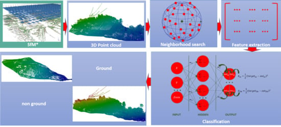
Four study areas were defined, two for calibration and two for validation. They are located in the Srem and Kolubara District, western Serbia. The validation area (Figure 1A,B) was located at the confluence of the Bosut and Sava Rivers, Municipality of Sremska Mitrovica, Republic of Serbia. Validation area (A) is located at river banks and has high terrain discontinuity. It is covered by water bodies (4.3%), buildings (2.5%), low vegetation (70.4%), medium vegetation (2.3%), high vegetation (7.6%), roads (2.1%), and embankment (2.7%). Validation area (B) is covered by high mixed vegetation (4.3%), agricultural fields and grassland (65.1%), urban areas (8.1%), roads (2.3%), embankment (1%), and bushes (1.4%). Both validation areas are mainly flat, because the highest DEM accuracy for flood modeling needs to be provided in flat areas. On the other hand, different land cover classes were chosen to compare the algorithm performance in different environmental scenarios.
This study used LiDAR and UAV data, which were collected over the areas shown in Figure 1. LIDAR data was collected over the areas A, B, C, and D, (Figure 1) and UAV data over the areas A and B. LiDAR data were used to calibrate the algorithm to obtain the DEM, as well as to test the influence of using balanced/imbalanced data when calibrating it. Once the algorithm was tested and validated, it was applied to the UAV data. The following paragraphs describe both LiDAR and UAV data sets.
Calibration (training) sample points were selected from a large number of point clouds with different terrain complexities. The training area in Figure 1C represents the steep terrain covered by dense vegetation, while area (D) represents the flat terrain covered by mostly agricultural fields and built up areas. Table 1 summarizes the data used in this study.
The LiDAR data were captured on 1 December 2017 with an average point spacing of 5.4 cm. The flying height, during the capturing of the LiDAR data, was approximately 200 m above ground level. The aircraft speed was 45 kn. Maximum scan angle was set to 60°. The list of instruments used for LiDAR data acquisition is presented in Table 2.
The UAV survey was conducted in April 2018 using a WingtraOne drone fitted with a 42 MP Sony RX1RII camera (Table 3). The GCPs are required in order to register the results into a reference coordinate system (WGS84/UTM34, EPSG: 32634). Thirteen GCPs were distributed over the study area. The GCP consists of visible targets (1 m × 1 m red crosses). The GCPs were surveyed using a RTK GPS receiver and GNNS permanent network of Serbia (AGROS). The average point density of UAV point cloud is 160 points per square meter.

3. Methods

LiDAR data were used to calibrate the algorithm to obtain the DEM, as well as to test the influence of using balanced/imbalanced data when calibrating it. Once the algorithm was tested, it was applied to the UAV data. Therefore, the following workflow was applied (Figure 2):
(1)
LiDAR point cloud: calculation of the contextual information for each point by considering the spatial arrangement of all points inside the local neighborhood,
(2)
LiDAR point cloud: feature extraction,
(3)
LiDAR point cloud: calibration and supervised classification (ground and non-ground points) using the deep back propagation neural network (BPNN)
(4)
Accuracy assessment of the LiDAR point cloud classification
(5)
Application to the UAV data
  • Create the UAV point clouds (from overlapping images and using the SfM algorithm)
  • UAV point cloud: feature extraction (the same as (2))
  • UAV point cloud: calibration and supervised classification (ground and non-ground points) using the deep back propagation neural network (BPNN) (the same as (3))
  • Accuracy assessment of the UAV point cloud classification (the same as (4))
(6)
Accuracy assessment of the LiDAR and UAV derived DEMs
(7)
Flood risk assessment using the created DEM.
The next paragraphs explain each step in more detail.

3.1. Point Cloud Generation using SfM Algorithm (UAV Data)

The SfM algorithm was applied to the set of UAV images acquired from multiple viewpoints to reconstruct the 3D geometry of objects and surfaces, and to transform them into a point cloud. The workflow consisted of three main steps, described below.
In the first step, SfM used scale invariant feature transforms (SIFT) to detect and describe local features (key points) that are invariant to image scaling, orientation, affine distortion, and changes in illumination conditions, and can be matched across multiple images using the RANdom SAmple Consensus (RANSAC) method [13]. Because we used the customer grade digital camera, which does not carry a GPS and IMU sensor that can collect data with sufficient accuracy, the intrinsic orientation parameters are neither known nor stable. To overcome these problems, the bundle block adjustment of matching key points was applied to compute the extrinsic camera (position and orientation) of each camera exposure station [30]. Also, the bundle adjustment simultaneously estimated the 3D coordinates for a sparse, unscaled point cloud and intrinsic camera parameters (focal length and two radial distortion parameters).
In the second step, the initial value of camera parameters and 3D point cloud were optimized by minimizing of a non-linear cost function that reflects the measurement and re-projection errors [11]. The GCP points, established before the survey, were used to georeference the SfM derived from the point cloud using the seven parameter Helmert transformation. For the seven parameter transformation, a minimum of three GCP need to be used. In this case, 13 GCP were used. As a third and final step, the multi-view stereo (MVS) image matching algorithm used the output of the bundle adjustment to build a dense 3D point cloud.

3.2. Neighborhood Search and Feature Extraction (UAV and LIDAR Point Clouds)

Two approaches can be used to define the local 3D neighborhood of a given 3D point X R 3 : geometric search and k-nearest-neighbor search. The most commonly used method is the spherical neighbored definition, where the local neighborhood is formed by all points in a sphere defined by a fixed radius. Geometric search can be based on a cylindrical neighborhood definition, where the local neighborhood is formed by all 3D points whose 2D projection onto the ground plane is within a fixed radius circle [31]. In the k-nearest neighbor search, the local neighbors are the fixed k nearest neighbors from the query point. All those methods are defined by one parameter, which is represented by either a radius or several nearest neighbors and can be derived based on prior knowledge about data. Because of a significant impact on local neighborhood and feature extraction, it is expected that the different neighborhood types and different parameters can have a significant influence on the classification result. Weinmann et al. [32] analyzed the behavior of standard 2D and 3D geometric features for different neighborhood types. Derived features were used to evaluate three classifiers for a different classification task. In that work, the results showed that the spherical neighborhood with a radius of 1 m provided high classification accuracy for each classifier. Therefore, in this research, we utilized the spherical neighborhood. After that, the neighborhood search, performed for each 3D point, was described as follows: for a given point cloud P = { X 1 , , X n } in a three-dimensional Euclidean vector space, those points X P that are located in the sphere defined with a center in query point X i and fixed radius represent local neighborhood of point X i . A kd-tree, binary tree based on a hierarchical subdivision of space by splitting hyperplanes that are orthogonal to the coordinate axes [33], is widely used for nearest neighbor search in computer sciences. The ckd-tree, defined as in the work of [34], finds 3D neighbors for 15,000 points 20% faster than kd-tree, and thus is used in this study.
Thus, in this work, the neighborhood search was performed using ckd-tree implemented in the Python programing language. The spherical neighborhood definition with radius of 1 m was set, and for each query point X i , minimum, maximum, and mean height in the local neighborhood was extracted. Then, difference values between the height of query point z i and z m a x , z m e a n and z m i n , as well as the height range, were calculated for each point. In addition to geometric features, the intensity value was also used. The intensity for LiDAR data was defined as the return strength of the laser pulse, while the intensity of UAV data is calculated from red green blue (RGB) colors of the point according to the following expression: I n t e n s i t y U A V = 0.21 × R e d + 0.72 × G r e e n + 0.07 × B l u e .

3.3. Classification of the UAV and LIDAR Point Clouds Using a Back Propagation Neural Network (BPNN)

Each point of the point cloud was classified as ground or non-ground using the back propagation neural network algorithm. For the main characteristics of BPNN, see the work of [35]. The task of classification was to predict label y for a given input x. The input consisted of eight layers (obtained in step 3.2.): three global geometric features (Xi, Yi, Zi), four extracted features from local neighbored (Zi-Zmin, Zi-Zmax, Zi-Zmean, Zmax-Zmin), and intensity. During the forward-passing, given input features x and a network with weights W, bias b and hyperbolic tangent (tanh)activation function the output of each layer h are defined as in Equation (1).
h = d = 1 D W d T × x d + b
Next, a loss was calculated as the negative log-likelihood between the prediction and the true label. The closer the prediction to the true label for each sample, the smaller the loss would be. The loss function was minimized by adjusting all of the parameters in the network using back-propagation. The learning was performed by adam, a stochastic gradient-based optimizer proposed by the authors of [36]. The selected activation function and optimizer provided the highest accuracy among tested combination, that is, sigmoid, rectified linear unit (relu), tanh, adam and stochastic gradient descent (sgd). The maximum number of epochs was set to 400, the learning ratio was 0.0001. The output consisted of labeled points, with the labels corresponding to the classes defined in training set (i.e., ground and non-ground).
The calibration data sets (C and D) were split into 70% for training and 30% for testing. A total of 5,612,957 labeled points were used to train the neural network in this study. The validation, training, and testing ground truths were labeled using automatic filtering implemented in TerraScan software and post manual editing.
Although point clouds offer large point counts in absolute terms, they contain large class imbalance. A dataset is imbalanced if the classes are not approximately equally represented. This is because of the natural ground and non-ground imbalance presented in both urban and rural environments, as well as in steep and flat terrain. The largest imbalance was noticed in area C covered by dense vegetation and objects (Table 1). The class imbalance can compromise the process of NN learning, because the model tends to focus on the prevalent class and ignore the rare events [37]. Therefore, and in order to compare the results of using imbalanced and balanced data sets to obtain ground points and DEM, in addition to the initially imbalanced C and D point clouds, three balanced data sets per point cloud were created using different re-balancing methods. The first data set (BU) was balanced by randomly removing data from the non-ground class (i.e., under sampling the non-ground class), so that its ratio approaches the ground class ratio; this strategy reduced the original data set by 75%, so that the final BU data set consisted of 1,403,696 points. The second balanced data set was obtained by oversampling (BO), where the representatives of the least represented class were replicated, creating additional 4,209,261 points (reaching a total number of 9,822,218 points in the BO dataset). As the data are just replicated, oversampling can lead to over-fit to small data samples; therefore, the combination of undersampling and oversampling was also tested (BOU). This third method was applied to balance the dataset, and in this case, the number points of ground class increased by 300% (4,211,088 points created), while the non-ground class was reduced by 50%. In all the balanced datasets, the class ratio (ground, non-ground) was 50%. Once the three balanced datasets were created, all four data sets were standardized using the StandardScaler function [38].
The proposed approach was implemented in the Jupyter Notebook environment and Python programming language by using numpy, laspy, scipy, and sklearn libraries.

3.4. Accuracy Assessment

3.4.1. Point Cloud Classification

To determine the accuracy of the point cloud classification, overall accuracy, the most common metric for classifier evaluation, can be used to assess the overall effectiveness of the algorithm by estimating the probability of the true value of the class label. However, imbalance validation datasets can lead to wrong conclusions because one class is overrepresented and the other underrepresented, and thus the omission and commission errors (and the overall accuracy (OA)) are affected. Thus, precision, recall, and F1-score were calculated to provide a comprehensive assessment of the proposed approach. Precision computes the percent of points classified as ground that are really ground, while recall represents the fraction of correctly labeled ground points. In a perfect model, the precision and recall will be equal to one. The F1-score represents the harmonic mean of precision and recall in Equation (4) [39].
p r e c i s i o n = t p t p + f p ,
r e c a l l = t p t p + f n ,
where tp, fp, and fn are true positive, false positive, and false negative, respectively.
F 1 = 2 × r e c a l l × p r e c i s i o n r e c a l l × p r e c i s i o n
According to Equation (4), the F1-score will be null whenever the precision or recall is equal to null, while the value of the F1-score will increase proportionally to the increase of precision and recall. The higher value of F1-score indicates that the model performs better on the positive class [40].
In this paper, the overall accuracy, precision, recall, and F1-score were calculated for the two validation sets (A and B) (Table 1); for the imbalanced (original) dataset; and for the three rebalanced datasets (BU, BO, BOU), obtained in an analogous way to the BU, BO, and BOU datasets described for training and testing in Section 3.3.

3.4.2. Point Cloud and DEM Accuracy

The accuracy of UAV and LiDAR based point cloud was assessed by comparing the results with the true data (datasets A and B). Two methods were applied: DEM of difference (DoD) and cloud-to-cloud (C2C) method
DEM of difference (DoD) is the most common method of point cloud comparison. The classified LiDAR and UAV ground points were gridded to generate DEMs with a spatial resolution of 0.25 m and then differenced on a pixel-by-pixel basis, allowing the estimation of vertical uncertainty and the detection of change. Also, the root mean square error (RMSE) and the mean average error (MAE) of elevation measurements were computed by extracting the DoDs in 36,600 randomly created check points across the entire A and B study areas. The number of check points was defined in order to provide density of 1 point per m2.
As gridding a point cloud and generating a DEM involves an interpolation error, direct cloud to cloud differences were calculated using the C2C tool implemented in open source CloudComparer software [41]. This method also allows for assessing the spatial variability of cloud accuracy. For each point of the second point cloud, the closest point can be defined in the first point cloud based on different performing algorithms [42]. The output of applying this method is a point cloud that contains information about the absolute distance for each point along the three axes (X, Y, Z). On the basis of the absolute distance, mean absolute distance (MAD) and standard deviation (SD) were calculated.

3.5. Flood Risk Assessment

In order to assess the usability of the proposed approach and the UAV SfM point cloud for flood risk assessment, the inundation area was simulated by selecting the grid cell of the DEM that was lower than the projected water level and that was connected to an adjacent flooded grid cell or open water, which will thus indicate inundation [5,43,44]. Flood risk assessment was calculated at 12 different vertical levels. The vertical distance between levels was set to 0.5 m.

4. Results

4.1. Point Cloud Classification

The results of the accuracy assessment for ground class extraction from the LiDAR point clouds using deep learning based on backpropagation neural network are displayed in Table 4. The algorithm showed a stable performance among the different data sets. As a measure of classification accuracy, the F1-score is considered to show strong agreement when it is close to 1, while values close to 0 indicate a poor agreement. Therefore, all data sets (original, BU, BO, BOU) provided ground point classifications with a strong agreement with the true data, as indicated by the low number of false positives and false negatives. The lowest F1-score in the testing phase was obtained for the ground class in the imbalanced data set, as only 71% of the ground points were correctly classified by the algorithm (recall: 0.71), while for the balanced datasets, the recall values were between 0.86 and 0.93.
For the validation, all the balanced datasets showed low precision (<0.4) and high recall (>0.8) for the ground point class, and high precision (>0.9) and low recall (<0.5) for the non-ground points. According to these values, in the balanced data sets, the algorithm produced a low number of false negatives, but high number of false positives. As a result, the balanced data sets produced a significantly lower F1-score for ground class in the validation phase, compared with the testing phase (0.90 vs. 0.53). The imbalanced data set provided stable metrics values between the validation and testing phase (0.78 vs. 0.79 F1-score for the ground class).
Taking into account the results presented in Table 4 and as discussed in Section 5, the classified imbalanced LiDAR point cloud gathered on the validation areas (Figure 1A,B) was used for the next sections (production of DEM, accuracy assessment, and flood risk assessment). Thus, the imbalanced UAV point clouds from study sites A and B were used for DEM production, accuracy, and flood risk assessment.

4.2. Spatial Variability of UAV and LiDAR DEM Accuracy

The DoD method was used to calculate total elevation discrepancies between the ground truth and LiDAR and UAV DEM. We used the residuals to estimate the MAE and RMSE. As MAE is a measure of DEM accuracy and is used to identify the overall bias in the data, the results showed that the classified LiDAR data tended to underestimate the elevation by an average of 5 cm (Table 5), while the UAV data overestimated the elevation by an average of 28 cm (Table 5).
In addition, the examination of individual cross sections at different locations across the study area was done in order to better understand the influence of land use/land cover classes in DEM accuracy. The results of the comparison are presented in Figure 3. In the case of the LiDAR DEM, the profiles were coincident or within a few centimeters of the true data (Figure 3a,b,d). The largest distance was noticed in the river bed (Figure 3c). For the UAV DEM, elevation differences in the river bed and area covered by dense vegetation (Figure 3b,c) were the largest, while the smallest elevation difference was obtained for bare land (Figure 3d).

4.3. Accuracy of UAV and LiDAR Point Clouds (C2C Method)

The distance between the reference (true point cloud) and target (LiDAR and UAV) point clouds was calculated using the C2C tool. The spatial distribution of the results of the C2C comparison along the Z axis for the LiDAR and UAV point clouds are shown in Figure 4. The MAD and the SD along the Z axis between the true point cloud and the LiDAR point cloud were significantly lower than when the UAV point cloud was compared (i.e., 0.002 m vs. 0.113 m, and 0.03 m vs. 0.392 m, respectively). The range of absolute distances for LIDAR was –1.28 to 4.18 m, smaller than for the UAV point cloud (–5.12 to 3.87 m).
In order to better understand those results, the number of points in different ranges of absolute error along the Z axis were computed (Table 6). Although the distance between true and LiDAR point clouds varied significantly, the C2C distance for 99.72% of the points was smaller than 5 cm, while for the UAV point clouds, the C2C distance was between 0.5 and –0.5 m for 87.21% of the points (Table 6).
Although the distance between true and LiDAR point clouds varied significantly, the C2C distance for 99.72% of the points was smaller than 5 cm (Table 6).

4.4. Flood Risk Assessment

The visual comparison of the inundation areas derived from true, LiDAR, and UAV data for different water levels is presented in Figure 5. These results show that the true and LiDAR data followed a similar pattern. The largest difference was obtained for the lowest water level. However, a strong pattern between true and UAV data was not obtained. The model performed the best for very high water levels, while the largest difference was achieved for the lowest water level. The relationship between the detected inundation area and water level is presented in Figure 6.

5. Discussion

5.1. Convenience of using Imbalanced or Balanced Datasets for Point Cloud Classification

Regarding the convenience of using balanced or imbalanced point could datasets for ground/non ground classifications, the comparison among the four LiDAR data set (Table 4) showed that the imbalanced data set was more accurate for ground point classification than the balanced ones in the validation phase.
On one hand, the results of the classification of the balanced data sets showed a strong agreement with true data for both classes in the testing phase (Table 4). In addition, the results showed that the method used for balancing the dataset (BU, BO, BOU) does not have significant influence in the algorithm accuracy (i.e., all the F1-scores were between 0.87 and 0.90). On another hand, and taking the BU dataset as an example of the three balancing methods, the F1-score strongly decreased in the validation phase when using the balanced data sets (ground: 0.90 vs 0.52; non ground: 0.89 vs 0.72). The values of recall and precision showed that the model is capable to detect ground points almost perfectly (recall: 0.97), but it also tends to misclassify the non-ground class as ground (precision: 0.37), producing a moderate F1 score (0.52).
To explain those results, it should be noted that during the test phase, for the balanced data sets, the artificially rebalanced training and test sets were used, producing high accuracies in the classification. Nevertheless, during the validation phase, the balanced training set was used for training the classifier, while the imbalanced (the real point cloud) validation set was used to test the classifier. Therefore, the training and validation sets had different distributions because of the bias introduced during rebalancing. It is well known that rebalancing modifies the prior training set and, consequently, biases the posteriori probability of a classifier [44]. The classifier trained this way tends to move the optimal separation boundary toward the majority class [45], so that more non ground points are classified into the ground class. This produced high recall and low precision for the balanced data set in the validation phase (Table 4). Additionally, oversampling can lead to over-fit to small data samples, while downsampling due to information loss [43] could reduce the classifier performance.
For the imbalanced data set, the performance of developed approach remained stable in both the testing and validation phase (Table 4). The high value of precision, recall, and F1-score indicated an almost perfect classification of the non-ground class. As a result of imbalance distribution and highly overlapping classes, the number of ground points correctly classified decreased [46], producing a lower F1-score (non ground: 0.95 vs ground: 0.78). The recall and precision value indicated that the model is highly trustable (precision: 0.86), correctly detecting 72% of the ground points. The values attained for the ground class were similar to the ones reported by Rizaldy et al. [25], who reached an average total error of 5.21%, with low type I (4.28%) and type II (14.28%) errors, meaning that more non-ground points were mislabeled. The higher type II error was explained by the number of non-ground data points in both samples being considerably lower than the number of ground points. Therefore, the validation recall value in the imbalanced data set could be explained in this case by the lower number of ground points. Heckel et al. [28] reached an overall classification accuracy of 95–98% and a mean F1-score of 0.70–0.74, which is similar to the results obtained in this study. However, the algorithm presented in this paper provided an almost complete ground classification (recall: 0.99, precision: 0.98, F1: 0.98), probably because of the low class overlapping, as linear separable classes are not sensitive to any amount of imbalance [46,47]. Because of the high degree of complexity of our data, the approach presented in this paper is more sensitive to imbalanced data sets then the approach shown in the work of [28]. The benefit of rebalancing is strongly dependent on the nature of the classification task and should be used only if the distribution of the generated and real data set will remain same.

5.2. Effect of the Land Cover Class on the Algorithm Performance and Elevation Accuracy

In relation to the accuracy in elevation, the LiDAR DEM had an RMSE of 0.25 m and an MAE of 0.05 m, while the UAV DEM had values of 0.59 m and –0.28 m, respectively (Table 5). In the work of [24], total classification error of LiDAR ground class was 2.9% over 40 various complex terrains, while RMSE ranged from 0.05 to 0.28 m. When the effect of the land cover/land use class in the accuracy of the DEM was analyzed (Table 5), it showed that the largest differences between both DEMs were obtained in the area covered by water bodies (RMSE of 0.37 m and 1.70 m for LiDAR and UAV DEM, respectively). The errors associated with this land cover were probably because of the fact that the training data did not include water bodies.
The second largest error for the UAV DEM was obtained for the high vegetation class (RMSE 1.00 m), with an average underestimation of 0.39 m, while the smallest ones were, in both cases, obtained for the low vegetation class (RMSE of 0.19 m and 0.23 m for LiDAR and UAV DEM, respectively). The RMSE for the vegetation classes was not significantly different in the LiDAR DEM, while for UAV DEM, the RMSE increased with the height of the vegetation class (Table 5). Along the same lines, the DoD examination of cross sections (Figure 3) and the results of the C2C comparison (Figure 4) also showed the increase of RMSE and MAE for UAV DEM with the increase of vegetation height. Those findings are in line with results presented in the work of [48]. In general, and for all land cover classes, the UAV DEM overestimated the elevation (MAE < 0), while the LIDAR DEM tended to underestimate it (MAE > 0).

5.3. Suitability of the Proposed Method to Produce DEM from UAV and LiDAR Data

In addition to the aspects discussed in the previous sections, and in order to determine the overall suitability of the proposed method to produce DEM for UAV and LiDAR data, the advantages and the shortcomings of this classification method are discussed below, taking into account the DEM accuracy.
The MAD and SD for the UAV point cloud (0.11 m and 0.39 m, respectively) were significantly higher than for the LiDAR data (0.002 m and 0.03 m, respectively). Those results are in line with the findings presented in the work of [19] and with results obtained comparing both point clouds using the DoD method (previous section).
Regarding the spatial variability of UAV and LiDAR DEM accuracy (Table 6), on the one hand, the large positive absolute distance along the Z axis between the LIDAR DEM and the true data (Table 6) was the result of the misclassification between the ground class and the points representing vegetation. The misclassification of some parts of the trees that were located near to the elevated embankment and the terrain break lines at the river banks produced the highest C2C distance (Figure 4a,c). Rizaldy et al. [25] reported a similar problem with the misclassification of non-ground points in the area where the ground surface is connected to the elevated bridge, because the boundary between the ground and the bridge is fuzzy owing to the gradual inclination of the road surface. As tree parts classified as ground were located at the same height as embankment, a similar explanation could be applied. On the other hand, large negative distances were noticed at the terrain brake lines near to water bodies (Table 4, Figure 4b, and Figure 5). This is not surprising because the training data set did not include this type of terrain and water bodies. Also, water absorbs most often the laser pulse causing dropouts, which could influence algorithm performance.
For the case of the UAV point cloud, the distances between true and compared data along the Z axis were between –5.12 and 4 m (Table 6). The location of the largest negative values (errors) in the UAV point cloud was the same as for those obtained for the LiDAR point cloud, although the distance values were much larger for the UAV points (Table 6). The same happened for the large positive values (Figure 4d). Nevertheless, the number of points with a distance larger than ±1 m accounted for just 2.16% of the total amount of points, which did not have a significant effect on the MAD and SD values. UAV equipped with a passive sensor (like in this case) does not have the ability to penetrate vegetation and, therefore, the accuracy of the UAV DEM is strongly affected by the land cover class (Table 6, Figure 4e,f). As the survey was conducted in April, when the vegetation was already in the growing season, most UAV points were within a distance of 0.25 m from the true data (Table 6), which could be close to the height of the vegetation at that time. Additionally, the 3D model creation using SfM is based on static scenes, and as trees and water are prone to movement, it represents a problem for the key point matching algorithm, causing dropouts, inaccurate elevation representation, and lack of data (Figure 4d).
The main advantage of the proposed method (raw point cloud classification and ground point filtering based on deep learning and NN) is the ability to classify raw point clouds without parameter settings and point to image conversion. Therefore, it is more efficient regarding computational cost and it is easier to use. The quality and size of training samples are crucially important for successful classification [49]. The algorithm will label the ground points of different terrain complexity with high accuracy if training data contain sufficient representatives of various terrain types and include all land covers. In the future, the geometric features based on the local structure tensor and more efficient neighbor finding algorithm should be tested.

5.4. Usability of the LiDAR and UAV SfM DEM in Flood Risk Mapping

The visual comparison of inundation areas showed a similar pattern between true and LiDAR DEM. On another hand, the UAV DEM tended to overestimate the terrain elevation (Table 5) and thus underestimated the inundation area (Figure 5) for all tested water levels (Figure 6). For both data sets, the largest differences too place for the lowest water level. This is expected as results of the C2C comparison (Figure 4), DoD (Table 5), and visual inspection suggest that the largest errors were related to water bodies. This was expected because of existing ground point classification error in the water bodies. For high water levels, all data sets performed similarly.
Taking into account the requested accuracy for flood inundation mapping according to European Union Flood Directive [5], the developed algorithm and both data sets (LiDAR and UAV) can be used for flood inundation maps generation. However, the requests of the Serbian law are satisfied by LiDAR data for all terrain types, while the DEM derived from UAV data can be used only for hilly areas. If the UAV data are gathered during the winter season, with a lower vegetation cover, this hindrance might be overcome.

6. Conclusions

NN and deep learning based methods have significant potential and can be used for automated point cloud classification and rapid DEM generation for flood risk mapping. In this paper, we presented and verified a method of point cloud classification and ground point filtering based on deep learning using NN. Filtering acquired point clouds based on deep learning using NN rapidly improved the process of ground classification of LiDAR and UAV data, producing DEM with the required accuracy for flood mapping according to European Flood Directive standards.
One of the advantages of using the approach presented in this paper is that users can feed the classifier with raw point clouds, avoiding data pre-processing. This is one of main advantages because it reduces the computational time and computer power, which is one of the biggest limitations when dealing with dense point clouds. Another advantage is that the process is fully automatized, so that it is straightforward for users to input the raw point cloud and create the digital elevation model. In addition, all the steps of the approach we present here for LiDAR data are implemented in Jupiter Notebook using Python programming language and free libraries, so it can be implemented free of charge on any computer.
The accuracy assessment of algorithm performance on balanced and imbalanced data sets showed that effectiveness of the rebalancing method depends heavily on the nature of the classification task, and can be used only if it provides same the artificially generated data as the same distribution real data.
The verification of the algorithm was done on LIDAR and UAV SfM point clouds and derived DEMs. On the one hand, the accuracy assessment of classified LiDAR point cloud showed that 99.72% of the points had differences smaller than 5 cm with the true data. On the other hand, differences with the UAV classified point cloud were much higher, with 87.21% of the points within a distance between 0.5 m and –0.5 m of the true data.
As minimum requirements for flood modeling in Europe are 10 m × 10 m horizontal and minimum 0.5 m vertical resolution, the results of the accuracy assessment of the UAV SfM point clouds and derived DEM confirmed that UAV SfM provides a derived DEM with a resolution and accuracy that are suitable for flood risk management. This DEM has some restrictions, and the essential remark is that the accuracy and precision of the SfM generated point cloud and DEM depend heavily on the characteristics of the surface, land cover, and model of acquisition. LiDAR is, therefore, the recommended technology for point cloud acquisition, but UAV SfM is also a suitable alternative for hilly areas.

Author Contributions

Conceptualization, G.J., M.G., F.A.T. and V.P.; methodology, G.J. and M.G..; software, G.J.; validation, V.P. and G.J.; investigation, G.J., M.G. and V.P.; writing—original draft preparation, G.J. and M.G.; writing—review and editing, F.A.T., G.J. and M.G.; visualization, G.J.; supervision, M.G. and F.A.T.

Funding

This research received no external funding.

Conflicts of Interest

The authors declare no conflict of interest.

References

  1. CRED; UNISDR. The Human Cost of Weather Related Disasters 1995–2015. Available online: https://reliefweb.int/sites/reliefweb.int/files/resources/COP21_WeatherDisastersReport_2015_FINAL.pdf (accessed on 17 May 2019).
  2. Directive 2007/60/EC of the European Parliament and of the Council on the Assessment and Management of Flood Risks. Available online: https://eur-lex.europa.eu/legal-content/EN/TXT/PDF/?uri=CELEX:32007L0060&from=EN (accessed on 25 May 2018).
  3. Ogania, J.L.; Puno, G.R.; Alivio, M.B.T.; Taylaran, J.M.G. Effect of digital elevation model’s resolution in producing flood hazard maps. Glob. J. Environ. Sci. Manag. 2019, 5, 95–106. [Google Scholar]
  4. Saksena, S.; Merwade, V. Incorporating the effect of DEM resolution and accuracy for improved flood inundation mapping. J. Hydrol. 2015, 530, 180–194. [Google Scholar] [CrossRef] [Green Version]
  5. EXCIMAP (European Exchange Circle on Flood Mapping). Handbook on Good Practice for Flood Mapping in Europe. 29–30 November 2007. Available online: http://ec.europa.eu/environment/water/flood_risk/flood_atlas/pdf/handbook_goodpractice.pdf (accessed on 25 May 2019).
  6. Rulebook for Determining Methodology for Flood Vulnerability and Flood Risk Mapping. Available online: http://www.rdvode.gov.rs/doc/dokumenta/podzak/Pravilnik%20o%20metodologiji%20za%20karte%20ugrozenosti%20i%20karte%20rizika%20od%20polava.pdf (accessed on 1 July 2019).
  7. Jovanović, M.; Prodanović, D.; Plavšić, J.; Rosić, N. Problemi pri izradi karata ugroženosti od poplava. Vodoprivreda 2014, 46, 3–13. [Google Scholar]
  8. Jakovljević, G.; Govedarica, M. Water Body Extraction and Flood Risk Assessment Using LiDAR and Open Data. In Climate Change Adaptation in Eastern Europe: Managing Risks and Building Resilience to Climate Change; Springer: Cham, Switzerland, 2019. [Google Scholar]
  9. Noh, S.J.; Lee, J.; Lee, S.; Kawaike, K.; Seo, D. Hyper-resolution 1D-2D urban flood modelling using LiDAR data and hybrid parallelization. Environ. Model. Softw. 2018, 103, 131–145. [Google Scholar] [CrossRef]
  10. Shen, D.; Qian, T.; Chen, W.; Chi, Y.; Wang, J. A Quantitative Flood-Related Building Damage Evaluation Method Using Airborne LiDAR Data and 2-D Hydraulic Model. Water 2019, 11, 987. [Google Scholar] [CrossRef]
  11. Smith, M.W.; Carrivick, J.L.; Quincey, D.J. Structure from motion photogrammetry in physical geography, Prog. Phys. Geogr. 2015, 1–29. [Google Scholar] [CrossRef]
  12. Eltner, A.; Kaiser, A.; Castillo, C.; Rock, G.; Neugirg, F.; Abellán, A. Image-based surface reconstruction in geomorphometry-merits, limits and developments. Earth Surf. Dyn. 2016, 4, 359–389. [Google Scholar] [CrossRef]
  13. Westoby, M.J.; Brasington, J.; Glasser, N.F.; Hambrey, M.J.; Reynolds, J.M. Structure-from-motion’ photogrammetry: A low-cost, effective tool for geoscience applications. Geomorphology 2012, 179, 300–314. [Google Scholar] [CrossRef]
  14. Gebrehiwot, A.; Hashemi-Beni, L.; Thompson, G.; Kordjamshidi, P.; Langan, T. Deep Convolutional Neural Network for Flood Extent Mapping Using Unmanned Aerial Vehicles Data. Sensor 2019, 19, 1486. [Google Scholar] [CrossRef]
  15. Hashemi-Beni, L.; Jones, J.; Thompson, G.; Johnson, C.; Gebrehiwot, A. Challenges and Opportunities for UAV-Based Digital Elevation Model Generation for Flood-Risk Management: A Case of Princeville, North Caroline. Sensor 2018, 18, 3843. [Google Scholar] [CrossRef] [PubMed]
  16. Schumann, G.J.P.; Muhlhausen, J.; Andreadis, K. Rapid Mapping of Small-Scale River-Floodplain Envronments Using UAV SfM Supports Classical Theoru. Remote Sens. 2019, 11, 982. [Google Scholar] [CrossRef]
  17. Govedarica, M.; Jakovljević, G.; Álvarez-Taboada, F. Flood risk assessment based on LiDAR and UAV points clouds and DEM. In Remote Sensing for Agriculture, Ecosystems, and Hydrology XX; SPIE: Berlin, Germany, 2018. [Google Scholar] [CrossRef]
  18. Liu, X.; Zhang, Z.; Peterson, J.; Chandra, S. The Effect of LiDAR Data Density on DEM Accuracy. 2007. Available online: http://citeseerx.ist.psu.edu/viewdoc/download?doi=10.1.1.458.4833&rep=rep1&type=pdf (accessed on 30 June 2019).
  19. Asal, F.F. Evaluating the effects of reduction in LiDAR data on the visual and statistical characteristics of the created Digital Elevation Models. In Proceedings of the 2016 XXIII ISPRS Congress, Prague, Czech Republic, 12–19 July 2016. [Google Scholar]
  20. Liu, X.; Zhang, Z.; Peterson, J.; Chandra, S. The effect of LiDAR data density on DEM accuracy. In Proceedings of the International Congress on Modelling and Simulation (MODSIM07), Christchurch, New Zealand, 2007; pp. 1363–1369. [Google Scholar]
  21. Thomas, I.A.; Jordan, P.; Shine, O.; Fenton, O.; Mellander, P.E.; Dunlop, P.; Murphy, P.N.C. Defining optimal DEM resolutions and point densities for modelling hydrologically sensitive areas in agricultural catchments dominated by microtopography. Int. J. Appl. Earth Obs. Geoinf. 2017, 54, 38–52. [Google Scholar] [CrossRef] [Green Version]
  22. Rashidi, P.; Rastiveis, H. Extraction of ground points from LiDAR data based on slope and progressive window thresholding (SPWT). Earth Obs. Geomat. Eng. EOGE 2018, 1, 36–44. [Google Scholar] [CrossRef]
  23. Axelsson, P. DEM generation from laser scanner data using adaptive TIN models. Int. Arch. Photogramm. Remote Sens. 2000, 33, 110–117. [Google Scholar]
  24. Hu, X.; Yuan, Y. Deep-Learning-Based Classification for DTM Extraction from ALS Point Cloud. Remote Sens. 2016, 8, 730. [Google Scholar] [CrossRef]
  25. Rizaldy, A.; Persello, C.; Gevaert, C.; Elberink, S.O.; Vosselman, G. Ground and Multi-Class Classification of Airborne Laser Scanner Point Clouds Using Fully Convolutional Networks. Remote Sens. 2018, 10, 1723. [Google Scholar] [CrossRef]
  26. Sofman, B.; Bagnell, J.A.; Stentz, A.; Vandapel, N. Terrain Classification from Aerial Data to Support Ground Vehicle Navigation. 2006. Available online: https://pdfs.semanticscholar.org/e94d/f03ec54e1c5b42c4ac50d4c8667d2e8cad6a.pdf?_ga=2.53795883.2092844519.1558797131-1702618147.1556638397 (accessed on 2 May 2019).
  27. Qi, C.; Su, H.; Mo, K.; Guibas, L.J. PointNet: Deep Learning on Pont Sets for 3D Classification and Segmentation. arXiv 2017, arXiv:1612.00593v2. [Google Scholar]
  28. Hackel, T.; Wegner, J.D.; Schindler, K. Fast semantic segmentation of the 3D point clouds with strongly varying density. In Proceedings of the 2016 XXIII ISPRS Congress, Prague, Czech Republic, 12–19 July 2016. [Google Scholar]
  29. Becker, C.; Hano, N.; Rosonskaya, E.; d’Angelo, E.; Strecha, C. Classification of Aerial photogrammetric 3D point clouds. arXiv 2017, arXiv:1705.08374v1. [Google Scholar]
  30. Turner, D.; Lucieer, A.; Watson, C. An Automated Technique for Generating Georectified Mosaics from Ultra-High Resolution Unmanned Aerial Vehicle (UAV) Imagery, Based on Structure from Motion (SfM) Point Clouds. Remote Sens. 2012, 4, 1392–1410. [Google Scholar] [CrossRef] [Green Version]
  31. Filin, S.; Pfeofer, N. Neighborhood systems for airborne laser data. Photogramm. Eng. Remote Sens. 2005, 71, 743–755. [Google Scholar] [CrossRef]
  32. Weinmann, M.; Mallet, C.; Jutzi, N. Involving different neighborhood types for the analysis of low-level geometric 2D and 3D features and their relevance for point cloud classification. In Proceedings of the 37. Wissenschaftlich-Technische Jahrestagung der DGPF, Würzburg, Germany, 08–10 March 2017; Kersten, T.P., Ed.; German Society for Photogrammetry, Remote Sensing and Geoinformatics: Hamburg, Germany, 2017. [Google Scholar]
  33. Friedman, J.H.; Bentley, J.L.; Finkel, R.A. An algorithm for finding best matches in logarithmic expected time. ACM Trans. Math. Softw. 1977, 3, 209–226. [Google Scholar] [CrossRef]
  34. Maneewongvatana, M.; Mount, D. Analysis of Approximate Nearest Neighbor Searching with Clusterd Point Sets. arXiv 1999, arXiv:cs/9901013v1. [Google Scholar]
  35. Alsmadi, M.; Omar, K.; Noah, S. Back Propagation Algorithm: The Best Algorithm among the Multi-layer Perceptron Algorithm. Int. J. Comput. Sci. Netw. Secur. 2009, 9, 378–383. [Google Scholar]
  36. Kingma, D.P.; Ba, J. Adam: A Method for Stochastic Optimization. arXiv 2015, arXiv:1412.6980v9. [Google Scholar]
  37. Kubat, M.; Matwin, S. Addressing the curse of imbalanced training sets: One-sided selection. In Proceedings of the 14th International Conference on Machine Learning (ICML), Nashville, TN, USA, 8–12 July 1997; pp. 179–186. [Google Scholar]
  38. sklearn. preprocessing. StandardScaler. Available online: https://scikit-learn.org/stable/modules/generated/sklearn.preprocessing.StandardScaler.html (accessed on 1 June 2019).
  39. Fawcett, T. An introduction to ROC analysis. Pattern Recognit. Lett. 2006, 27, 861–874. [Google Scholar] [CrossRef]
  40. Bekkar, M.; Kheliouane Djemaa, H.; Akrouf Alitouche, T. Evaluation Measure for Models Assessment over Imbalanced Data Sets. J. Inf. Eng. Appl. 2013, 3, 27–38. [Google Scholar]
  41. CloudCompare. Available online: https://www.cloudcompare.org/ (accessed on 5 June 2019).
  42. Lague, D.; Brodu, N.; Leroux, J. Accurate 3D comparison of complex topography with terrestrial laser scanners. Application to the Rangitikei canyon. J. Photogramm. Remote Sens. 2013, 82, 10–26. [Google Scholar] [CrossRef]
  43. Chen, C.; Liaw, A.; Breiman, L. Using Random Forest to Learn Imbalanced Data. Available online: https://statistics.berkeley.edu/tech-reports/666 (accessed on 21 July 2019).
  44. Dal Pozzolo, A.; Caelen, O.; Bontempi, G. When is undersampling effective in unbalanced classification tasks. In Machine Learning and Knowledge Discovery in Databases; Springer: Berlin, Germany, 2015. [Google Scholar]
  45. Dal Pozzolo, A.; Caelen, O.; Johnson, R.A.; Bontempi, G. Calibrating probability with under sampling for unbalanced classification. In Proceedings of the IEEE Symposium Series on Computational Intelligence, Cape Town, South Africa, 7–10 December 2015. [Google Scholar]
  46. Sun, Y.; Wong, A.K.; Kamel, M.S. Classification of imbalanced data: A review. Int. J. Pattern Recognit. Artif. Intell. 2009, 23, 687–719. [Google Scholar] [CrossRef]
  47. Japkowicz, N.; Stephen, S. The class imbalance problem: A systematic study. Intell. Data Anal. J. 2002, 6, 429–450. [Google Scholar] [CrossRef]
  48. Salach, A.; Bakula, K.; Pilarska, M.; Ostrowski, W.; Gorski, K.; Kurczynski, Z. Accuracy Assessment of Point Clouds from LiDAR and Dense Image Matching Acquired Using the UAV Platform for DTM Creation. ISPRS Int. J. Geo-Inf. 2018, 7, 342. [Google Scholar] [CrossRef]
  49. Kavzgoul, T. Increasing the accuracy of neural network classification using refined training data. Environ. Model. Softw. 2009, 24, 850–858. [Google Scholar] [CrossRef]
Figure 1. Study area location. Four study sites (A, B, C, D). The coordinate reference system is WGS84/UTM34 34N EPSG 32634.
Geosciences 09 00323 g001
Figure 2. Workflow. Note: the same steps for light detection and ranging (LiDAR) and unmanned aerial vehicle (UAV) data are shaded with dark blue color. SfM, structure from motion, DEM, digital elevation model.
Geosciences 09 00323 g002
Figure 3. Comparison true data and LiDAR and UAV data using the proposed classification method. The green points represent the non-ground class, while the orange points represent the ground class. Profiles were created over different land cover classes ((a) built up areas; (b) dense vegetation; (c) water; (d) bare earth) based on DEM with a spatial resolution of 25 cm. The red, blue, and green lines represent the true, LiDAR, and UAV data, respectively.
Geosciences 09 00323 g003
Figure 4. Visual comparison of cloud-to-cloud (C2C) absolute distance along the Z axis. Left column represents the distance between LiDAR and true data ((a,c) represents maximum positive difference, (b) maximum negative distance), while the right column represents distance between UAV and true data ((d) maximum positive distance, (e,f) illustrate relationship between spatial variability of distance and land cover class i.e., grass and shrubs respectively).
Geosciences 09 00323 g004
Figure 5. Visual comparison of detected inundation area based on the water level and true, LiDAR, and UAV data.
Geosciences 09 00323 g005aGeosciences 09 00323 g005b
Figure 6. Relationship between the detected inundation area for different data sources and water levels.
Geosciences 09 00323 g006
Table 1. Light detection and ranging (LiDAR) data used in the study.
AreaTypeNumber of Points Ground [%]Non Ground [%]
AValidation2,804,72623.276.7
BValidation4,419,52017.882.2
C Algorithm calibration 3,801,4128.191.9
DAlgorithm calibration1,811,54523.676.4
Table 2. Instrument mapping list used for LiDAR point cloud acquisition.
TypeTitle 2
LiDARLMS-Q680i-Full Waveform Analysis with settable frequency up to 400,000 Hz, with field of view of 60°, and a divergence of 0.5 mrad beam; Class 3R
Navigation systemIGI CCNS5 + Aerocontrol (positioning and navigation unit data storage); Inertial Measurement Unit (IMU) IIf (inertial unit—400 HZ); GPS a 2 HZ (Novatel antenna 12-channel L1/L2).
Cameran.1 Metric Camera Digicam-H39 (39 Mpixels)
Thermal CameraVariocam thermal sensor system with a detector of 1024 × 768 pixels and the spectral range from 7.5 to 14 μm.
Table 3. Unmanned aerial vehicle (UAV) data survey details.
Image Resolution [MP] Number of GCPAttitude of Image Capture [m]Forward Overlap [%]Side Overlap [%]Ground Resolution [cm pix−1]
421315070702.7
Table 4. Results of the accuracy assessment for the LiDAR datasets and the proposed classification method. BU (data set balanced by undersampling of non-ground class), BO (data set balanced by oversampling of ground class), BOU (data set balanced by oversampling of ground class and undersampling of non-ground class).
PrecisionRecallF1-scoreOA [%]
TestBUNon-ground0.900.890.8989.53
Ground0.890.900.90
BONon-ground0.920.860.8989.77
Ground0.880.930.90
BOUNon-ground0.900.920.9189.68
Ground0.880.860.87
ImbalancedNon-ground0.920.980.9693.37
Ground0.890.710.79
ValidationBU Non-ground0.990.560.7264.80
Ground0.370.970.52
BONon-ground0.950.510.6660.81
Ground0.360.930.52
BOUNon-ground0.930.580.7164.52
Ground0.380.850.53
ImbalancedNon-ground0.930.970.9592.20
Ground0.860.720.78
Table 5. Accuracy of LiDAR and UAV digital elevation model (DEM) per land cover/land use classes (root mean square error (RMSE) and mean average error (MAE)) using the DEM of difference (DoD) method.
LiDARUAV
RMSE [m]MAE [m]RMSE [m]MAE [m]
All classes0.250.050.59−0.28
Water0.370.091.70−1.11
High vegetation0.200.031.00−0.39
Medium vegetation0.190.040.51−0.26
Low vegetation0.190.040.23−0.21
Bare land0.200.030.25−0.18
Built up areas0.270.060.28−0.27
Table 6. Distribution of points based on cloud-to-cloud (C2C) distance for LiDAR and UAV point clouds.
Absolute Distance along Z axis [m]Number of Points LidarPercent Lidar [%]Number of Points UAVPercent UAV [%]
–5.12 to –40021290.0282
–4 to –30016100.0213
–3 to –20011,4620.1517
–2 to –180.000519,7120.2608
–1 to –0.5520.0036275,6483.6471
–0.25 to –0.52920.0203680,8299.0079
–0.1 to –0.256000.0418789,88810.4509
–0.1 to –0.0513300.0925440,8205.8324
–0.05 to –0.0114,1050.9816242,4283.2075
–0.01 to 01,303,37490.702100
0 to 0.0167,0854.6685360,1294.7648
0.01 to 0.0543,0762.9976274,2413.6284
0.05 to 0.153670.3735400,2575.2957
0.1 to 0.2510560.07342,119,94228.0486
0.25 to 0.52790.01941,283,58016.9828
0.5 to 11760.0122580,2836.9696
1 to 2470.0032128,6561.5211
2 to 31090.007612,9800.1585
3 to 4260.001817780.0226
4 to 4.1810.000200

