1. Introduction
Ore deposits are generally formed by hydrothermal activity, which also forms various types of alteration zones in the vicinity of such deposits. Identifying alteration zones can clarify the mineralization mechanism and provides information indispensable for mineral resource exploration. The application of an alteration halo accompanied by the alteration of host rocks to the exploration of the Kuroko ore deposits produced many results in Japan (see, e.g., [
1]). It is important to identify the alteration zone in the exploration of porphyry copper deposits. More than 50% of global copper production is from porphyry copper deposits, making them the most important copper resource. The alteration zone of a porphyry copper ore deposit is relatively large and typically extends over several kilometers [
2].
The type of alteration zone varies with temperature and the chemical composition of the hydrothermal fluid and host rocks. The alteration minerals that form the alteration zone are diverse. However, the acidic alteration zone near a deposit consists of many alteration minerals which exhibit characteristic absorption peaks in the short-wavelength infrared (SWIR) region. This alteration zone often shows a concentric zonal structure, for which the center of mineralization can be estimated. The chemical compositions of samples collected in alternation zones can be analyzed in the laboratory. Alternatively, a portable spectrometer can be used to identify the characteristics of an alteration zone in the field, which greatly helps geological engineers to conduct on-site investigations. The Metal Mining Agency of Japan (MMAJ) [
3] developed an alteration mineral identification device called POrtable SpectrorAdiometer for Mineral identification (POSAM), which consists of a spectrometer and a hand-held computer that displays mineral identification results. It provides scores from the master database of absorption peaks identified using numerical calculation. The master database includes mineral names, basic total scores, wavelength position, tolerance range of absorption peak, sharpness of absorption, and other information. For conventional methods, researchers must create feature quantities. Diagnostic absorption peaks are then extracted from the obtained spectral reflectance data to identify minerals. However, inexpensive spectrometers may exhibit a wavelength shift, even after wavelength calibration. This shift may lead to an incorrect position being obtained for the absorption peak, possibly resulting in erroneous identification. The present study applied deep learning (DL) to the identification of alteration minerals to overcome the problem of wavelength shift. The ability to automatically identify alteration minerals from spectral reflectance will facilitate analysis for both experienced and new geologists. The proposed method will also be useful for the field verification of remote sensing data and may be applicable to the hyperspectral data obtained by air-borne or space-borne sensors.
Early DL algorithms required researchers to extract features for identification. The DL learns the data and the correlation between the extracted feature quantities. For spectra, the position, shape, and depth of an absorption peak are considered to be feature quantities. The extraction of feature quantities greatly depends on the researcher. Current DL algorithms can automatically extract feature quantities from data, eliminating the variation caused by researchers and enabling higher-order analysis. Despite progress in DL development, it is still unclear whether DL can be used for the identification of alteration minerals. The present study proposes a method for the identification of alteration minerals, based on a DL algorithm that automatically extracts feature quantities from the reflectance spectra. This study uses two DL methods, a multilayer perceptron (MLP) and a convolutional neural network (CNN), to identify alteration minerals. The performance of these methods in mineral identification is evaluated using 30 measurements of 24 alteration minerals used as indicators in hydrothermal exploration.
Tanabe et al. [
4] used a forward-propagation neural network (NN) with three layers for the identification of alteration minerals with a dedicated neuro-board and identified six mineral species. This was a trial study, with the input layer limited to 255 neurons and only an MLP used for comparison. Although the study showed that minerals could be classified into six kinds with almost 100% accuracy, the dedicated hardware board has limited further development. Montero et al. [
5] used a method similar to the Spectral Angle Mapper (SAM) method [
6], which is a popular mineral identification method used for multispectral or hyperspectral image data. The study used data processing methods, such as the Fast Spectral Identification Algorithm (FSTSpecID), continuum removal method, smoothing, and derivation, followed by feature matching using the center wavelength, absorption depth, spectral contrast, full width at half maximum, and symmetricity of the absorption features of the alteration minerals in a multi-dimensional coordinate system. Then, a vectorized and standardized reference spectral library was used for identification. This method can be regarded as a classic method, in the sense that a researcher must provide the feature quantities. Ishikawa and Gulick [
7] proposed a robust and autonomous mineral identification method using the Raman spectrum database RRUFF™. They showed that mineral classifiers developed with artificial NNs could be trained to accurately distinguish the major minerals which characterize igneous rocks using Raman spectra. These minerals include olivine, quartz, plagioclase, potassium feldspar, mica, and some pyroxenes. The classifier showed an average accuracy of 83%. Quartz, olivine, and pyroxene were classified with 100% accuracy. It is difficult to distinguish plagioclase from potassium feldspar in Raman spectra and RELAB reflection spectra because of their chemical similarity. For example, 77% of the plagioclase spectrum was incorrectly classified as potassium feldspar with the RRUFF™ test set. Liu et al. [
8] applied DL to Raman spectra in the RRUFF ™ database. The RRUFF™ project has developed technologies to create high-quality spectral data from distinctly characterized minerals and to share this information with the world. The project has been used to compare methods, such as CNN and the support vector machine (SVM) [
9]. Although baseline correction is often used in Raman spectroscopy, it does not show good results with CNN (which is generally better than SVM for spectral identification). In Raman spectra, the spectral shapes are almost the same; only wavelength position and the intensity of spectral features can be used for identification. In contrast, as this study deals with the shape of absorption features, in addition to the wavelength position and intensity, the problem to be solved in this study is more complicated.
Spectral identification with DL has only been applied to Raman spectroscopy, as it is difficult to create a large learning dataset. The present study applies DL to the identification of alteration minerals with automatic extraction of feature quantities from reflectance spectra.
2. Data
2.1. Datasets of Target Minerals
Spectral reflectance data were collected from various sources, including the spectral library of the U.S. Geological Survey [
10] and spectral data provided by the Geological Survey of Japan [
11,
12]. In addition, reflectance spectra of 24 kinds of alteration mineral were measured using a field spectroradiometer (FieldSpec4Hi-Res) by the authors.
The reflectance spectra of 24 alteration minerals, measured more than 30 times, were used to develop an identification model based on DL.
Table 1 shows the 24 target minerals used in this study. The selected alteration minerals were alunite, anhydrite, calcite, chlorite, dickite, dolomite, epidote, gibbsite, goethite, gypsum, halloysite, hectorite, illite, jarosite, kaolinite, montmorillonite, muscovite, natrolite, nontronite, phlogopite, pyrophyllite, rhodochrosite, talc, and vermiculite.
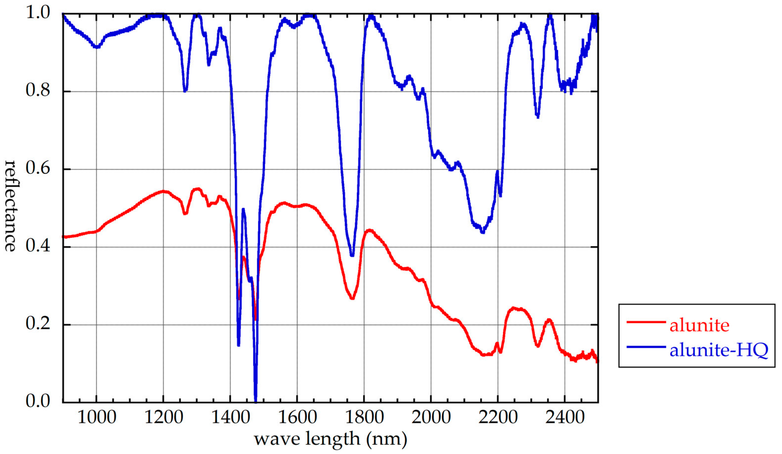
As pre-processing, all spectra were converted to reflectance data with a 1 nm interval. The wavelength region used for DL was set to 800–2500 nm (in the SWIR region), where the alteration minerals have distinctive absorption features. For DL with the hull quotient (HQ), the noisy parts at the ends of the 800–2500 nm range were not used; the wavelength range was thus 1000–2400 nm. HQ is a waveform data processing method for understanding the wavelength and intensity of the absorption features. The envelope curve on the side of the higher spectral reflectance was approximated by several straight lines, expressed by the quotient of the hull value and the measured value. This is useful for visually emphasizing small absorption features. The HQ process is normally performed using semi-automatic spectrum identification software.
Two datasets were created for the DL processing in this study. The first set was created using data for minerals found online, such as the spectral library of the U.S. Geological Survey. As these data were limited, the second set was prepared by collecting spectra of major hydrothermal alteration minerals using a field spectroradiometer (FieldSpec4Hi-Res) by the authors. The number of measurements of each mineral species was gradually increased to examine its effect on the accuracy rate. The minerals in dataset 1 (alunite, kaolinite, dickite, dolomite, gibbsite, gypsum, montmorillonite, muscovite, and natrolite) were measured 20 times, where 15 rounds were used for learning and 5 rounds were used for testing. The minerals in dataset 2 were measured 30 times, where 20 rounds were used for learning, and 10 rounds were used for testing.
2.2. Pre-Processing: Hull Quotient and Augmentation
DL was carried out with HQ for 30 measurements.
Figure 1 shows a comparison of reflectance spectra of alunite, obtained with and without HQ.
Using the spectral data collected, 50 spectra were amplified by adding random values in the reflectance direction and the wavelength direction. This process is called data augmentation. Fifty reflectance spectra from one sample were created by considering the following points:
- a)
Dispersion in the wavelength direction of the spectral measurements;
- b)
distance from the sample to a spectrometer, which causes a variation in the incident light intensity and, thus, affects reflectance; and
- c)
dispersion of each channel of the spectrometer for every 1 nm.
The wavelength direction was determined by measuring the deviations of the actual devices. For Augmentation Type1 (Aug Type 1), a random value for augmentation was placed with a maximum of 10% reflectance direction and a maximum of 10 nm in the wavelength direction. On the contrary, the random value added in augmentation for Aug Type 2 was less than half of Aug Type 1, and the noise was not recognized as an absorption peak after the HQ processing.
The data were increased 50-fold through augmentation. The total number of data points was 36,000.
3. Methods
3.1. Deep Learning
The perceptron, invented by Rosenblatt [
13], initially had many problems. Back-propagation was invented in the 1980s [
14], but development stopped due to its inefficient mechanisms. DL has a feature that develops multiple layers of artificial neurons, based on human brain circuits as a model, which learns by changing the weight of each neuron based on the input data, and becomes smarter as it repeats the analysis. DL processing consists of two steps: In the training step, a learning model is generated based on accumulated data and, in the scoring step, newly input data are classified and analyzed by applying the trained NN. DL algorithms will continue to evolve [
15]. Predictron [
16] and Deepforest [
17] are the state-of-the-art methods in this area. In this research, we reduced over-learning by frequent use of drop-out layers and the convergence was sped up by selecting an appropriate learning rate. All layer structures of our method were original. As a result, our method performed better than the previous methods. DL has led to advances in science and industry, with applications in self-driving cars, image analysis, and machine translation.
3.1.1. Multilayer Perceptron
A MLP has four or more layers of NN. Between the input and output layers, there are many dense layers and drop-out layers. Generally, the error-correction learning updates the connection weight, based on the relationship between the supervised signal of the input data and the output. In the original MLP, it was not possible to correct errors beyond the layer, so learning could not be done with multiple layers. The connection weight between the input layer and the intermediate layers was determined by a random number, and only the weight between the intermediate layer and the output layer was learned by error-correction. To avoid overfitting, it may be possible to prematurely abort, increase the number of training data, change the model to a simple one, and/or use drop-out. Drop-out is a way to invalidate hidden layer neurons with a certain probability in a network when learning. As a result, it is possible to learn automatically with different architectures each time.
The error back-propagation method was developed for the multilayer perceptron. The error function is important for back-propagation. Usually, the mean square error is used:
where
xi is the
i-th output of the network and
yi is the target value for the
i-th output. The weights are updated to minimize the mean square error.
When updating an MLP, it is necessary to calculate the updated weight of each parameter. The parameters to be updated are the weight and bias of each layer. The MLP obtains the updated weight of each parameter, based on the learning error. The error back-propagation method is used to obtain the updated weight of each parameter. Then, the parameters are updated using the gradient descent optimization method with the updated weight. For an MLP, although the learning time is relatively short, the number of parameters is large, and parameter adjustment is not easy. Also, an MLP tends to exhibit overfitting and is susceptible to noise, and its convergence is sometimes slow.
3.1.2. Convolutional Neural Network
A CNN consists of an input layer, a convolution layer, a pooling layer, a drop-out layer, a fully-connected layer, and an output layer. The convolution and pooling layers are repeated to form deep layers. A regular two-dimensional CNN (CNN2d) has a filtering layer and a max pooling layer, in multiple layers, and combines all layers at the end before output. As for this study, drop-out layers were mostly used as the model causes overfitting. Lawrence et al. [
18] reported the overfitting concept using approximation. According to this paper, as the order (and number of parameters) increases, the approximated function better fits the training data, but the interpolation between training points is very poor. A one-dimensional CNN (CNN1d) is a method of direct convolution with a filter size of 1 × 3 into the spectral reflectance.
Overfitting refers to a model that is too specific to a certain dataset (i.e., the model is not general). Avoiding overfitting is an important task for DL. CNN prevents the diffusion of errors by convolving and pooling layers between each layer, making the combination of layers rarely occur, so that overfitting does not easily occur, even with multiple layers.
Feature quantities extracted by a CNN are invariant to a small position change caused by convolution and pooling processing. The dataset used for DL was divided into training and test datasets. Learning was performed with the training dataset, and the generalization ability of the trained model was evaluated with the test dataset. CNN automatically updated the weights, so that the value of the loss function became smaller.
3.2. Study Setup
In this study, MLP and CNN were the chosen DL methods for alteration mineral identification. Spectral reflectance data can be regarded as a series of values in one-dimensional space. The MLP method is suitable for analyzing such one-dimensional data. Spectral reflectance data are often drawn as a two-dimensional image, with reflectance on the vertical axis and wavelength on the horizontal axis. The CNN method is suitable for analyzing such two-dimensional images.
DL is a multilayer NN, modeled on the neural circuits of a human brain. The basic part of a multilayer NN is called a perceptron, which functions as a human nerve cell. The perceptron identifies the shape of a spectral pattern and identifies features by extracting them without convolution.
A CNN identifies the shape of an object through convolution, such as edge detection. It extracts feature quantities for each region through filtering. CNN was used in this research because of its excellent image recognition capability.
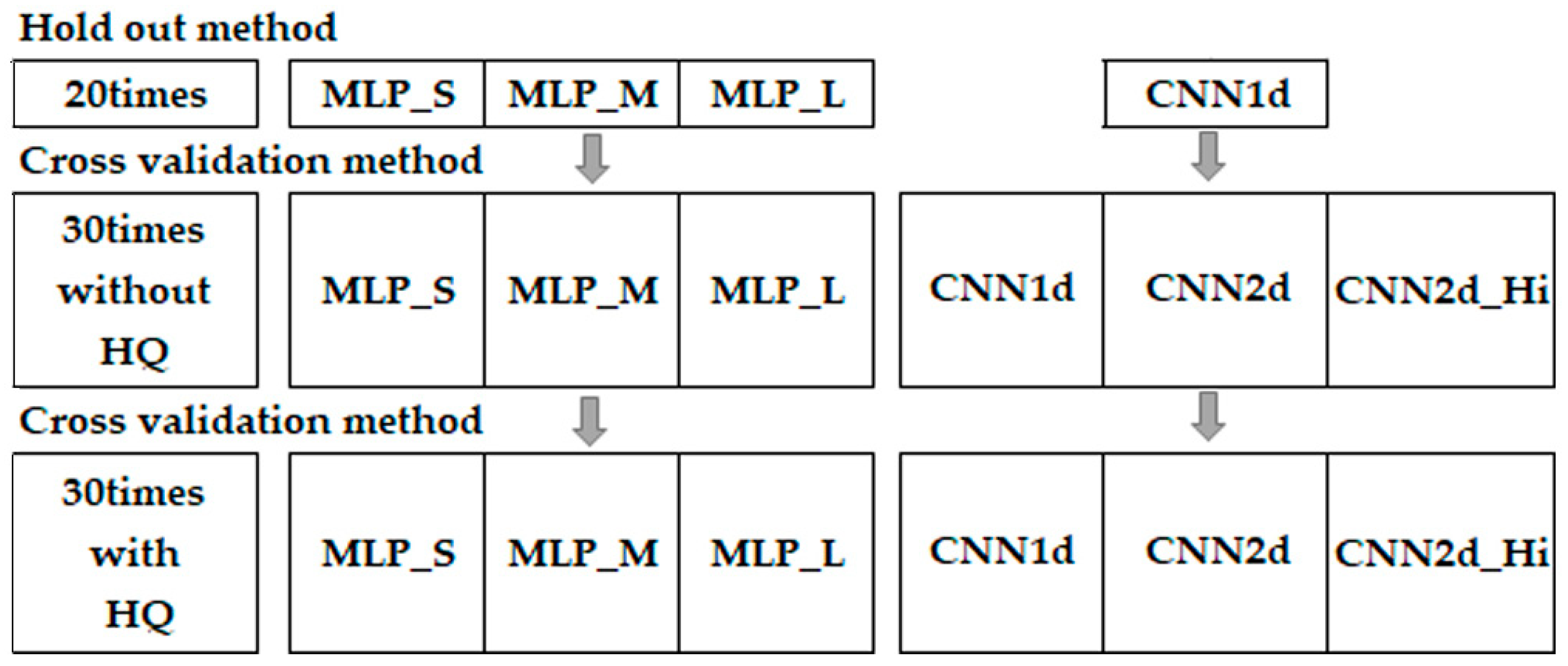
A flowchart of this research is shown in
Figure 2. For MLP, three-layer configurations were evaluated—namely, MLP Small (MLP_S), MLP Medium (MLP_M), and MLP Large (MLP_L)—to evaluate the effect of NN layer number on the identification of alteration minerals. MLP_S consisted of 4 dense layers and 3 drop-out layers, MLP_M consisted of 9 dense layers and 8 drop-out layers, and MLP_L consisted of 13 dense layers and 12 drop-out layers. For CNN, both CNN1d and CNN2d were evaluated. CNN1d applied a 1 × 3 filter to the reflectance spectra. As the reflectance was on the order of 1 nm, it was considered to be one-dimensional. CNN2d was used for image identification. It was evaluated with coarse (430 × 286) resolutions as CNN2d and fine (1773 × 229) resolutions as CNN2d_Hi. The number of measurements of data was evaluated by increasing the number of tests in two stages; namely, 20 and 30 measurements. For 30 times of measurements, HQ was conducted, and K-fold cross-validation tests were applied to the results. This is a useful method when training and test datasets are measured using different spectrometers with different spectral resolutions, and the data are not sufficiently shuffled. For each process, the relationship between the value of the loss function and the value of the accuracy, as well as the number of epochs, is indicated. The loss function is an indicator of overfitting. Learning is done by modifying the weights and biases so that the output layer has the correct value. The epoch number is the number of times that learning is repeated.
3.3. Evaluation Method for Model
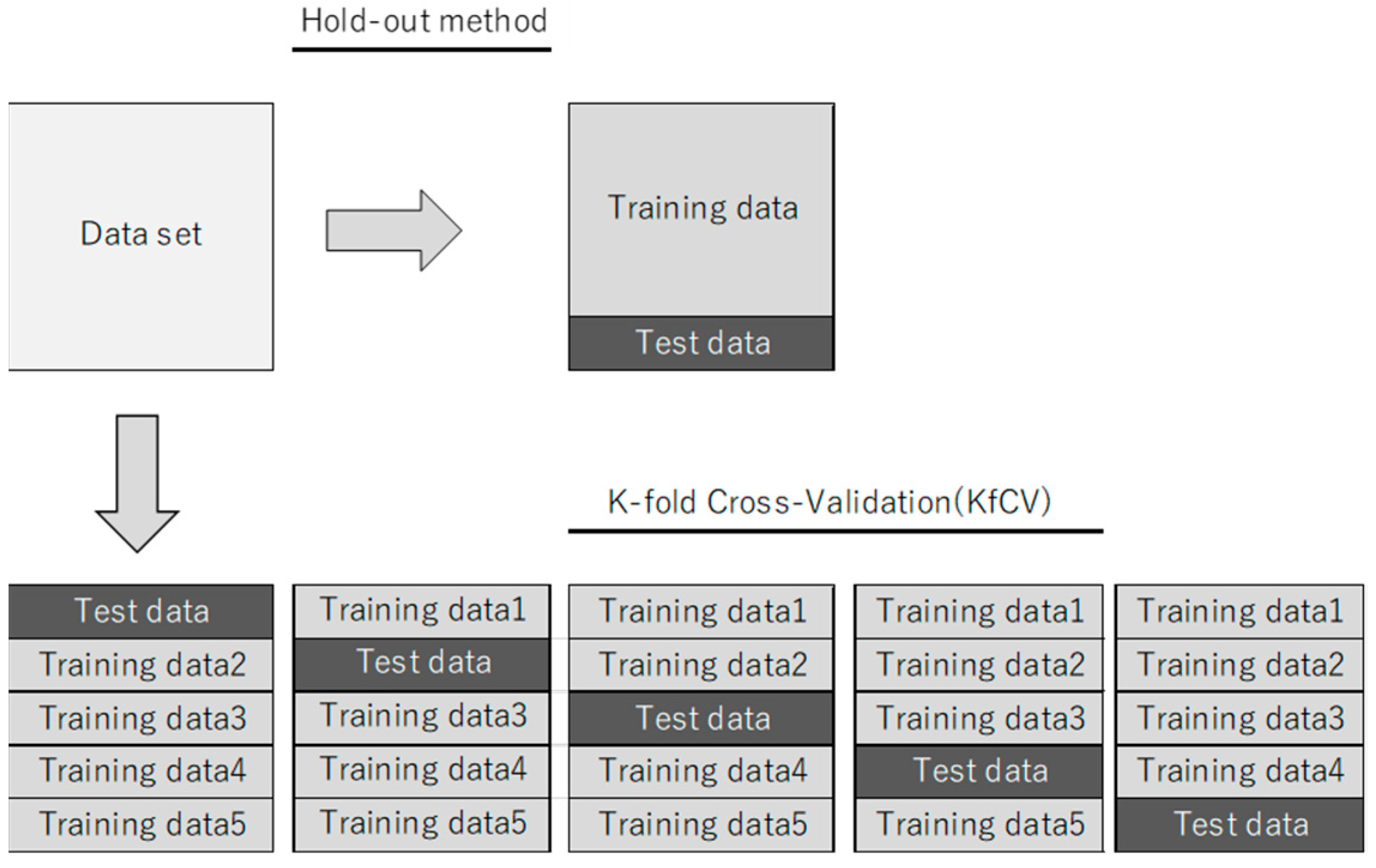
Commonly-used methods for evaluating a DL learning model are the hold-out method and the K-fold cross-validation method. The hold-out method was applied to a dataset with 20 mineral species, and K-fold cross-validation was applied to a dataset with 30 mineral species.
The hold-out method evaluates a model by dividing the data into learning data, used to create a model, and test data, used to evaluate the model. Learning data cannot be used to evaluate the generalization capability of a model.
K-fold cross-validation divides the data into K equal parts (K = 5, in this study). One part is used as a test case, and the remaining K-1 parts are used as training examples. K-fold cross-validation evaluates each sample group as a test case (i.e., there are K evaluations). An estimate was obtained from the average, derived from the results of such an examination done K times. When the data volume is small, depending on how test data are selected, there is a high possibility that a large error will occur in the estimation. In such a case, the K-fold cross-validation method is effective, and it is more reliable than the hold-out method in the evaluation results. As the evaluation is repeated and data are crossed and then averaged, specific data bias in the test data is avoided.
Figure 3 shows the evaluation methods for DL.
3.4. Hardware and Software Specifications
The following hardware and software were used in this study:
Hardware:
CPU: Intel Core i7-6700 3.4 GHz
Memory: 64 GB
GPU: NVIDIA GeForce GTX 1080 Ti
Software:
OS: Ubuntu 16.04, Windows 10
NVIDIA Docker (Ubuntu)
Python 3.6.3, Keras 2.1.0, Tensorflow 1.4.0
Regarding the time complexity, a simpler model can reduce the number of parameters and calculation time. However, the calculation time of a CNN still exceed one day. The spatial complexity was greatly streamlined with the advent of NVIDIA GeForce GPUs and 64GB minimum memory.
4. Results
4.1. Deep Learning without HQ
In this study, we evaluated the accuracies of MLP_S, MLP_M, and MLP_L in the identification of alteration minerals. We tried to determine which layer configuration was most suitable. In addition, CNN1d and CNN2d were evaluated. The hold-out method was used for 20 measurements, and K-fold cross-validation was used for 30 measurements. Aug_Type1 was used, because the noise was considered to be somewhat large (see
Section 2.2). Identification of alteration minerals was carried out with 23 minerals, except for vermiculite. The results of 30 measurements of the minerals are presented below.
Table 2 shows the layer structure of MLP_S. Even with such a simple structure, the MLP is characterized by a large number of parameters.
The number of parameters is source_N_number × destination_N_number + n terms. For example, the number of parameters of dense_1 is 1701 × 512 + 512 = 871,424 (where 1701 is derived from the range 900–2500 nm). Dense refers to a fully-connected layer.
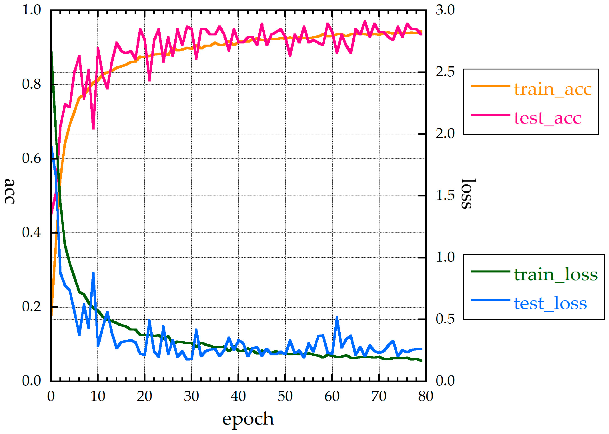
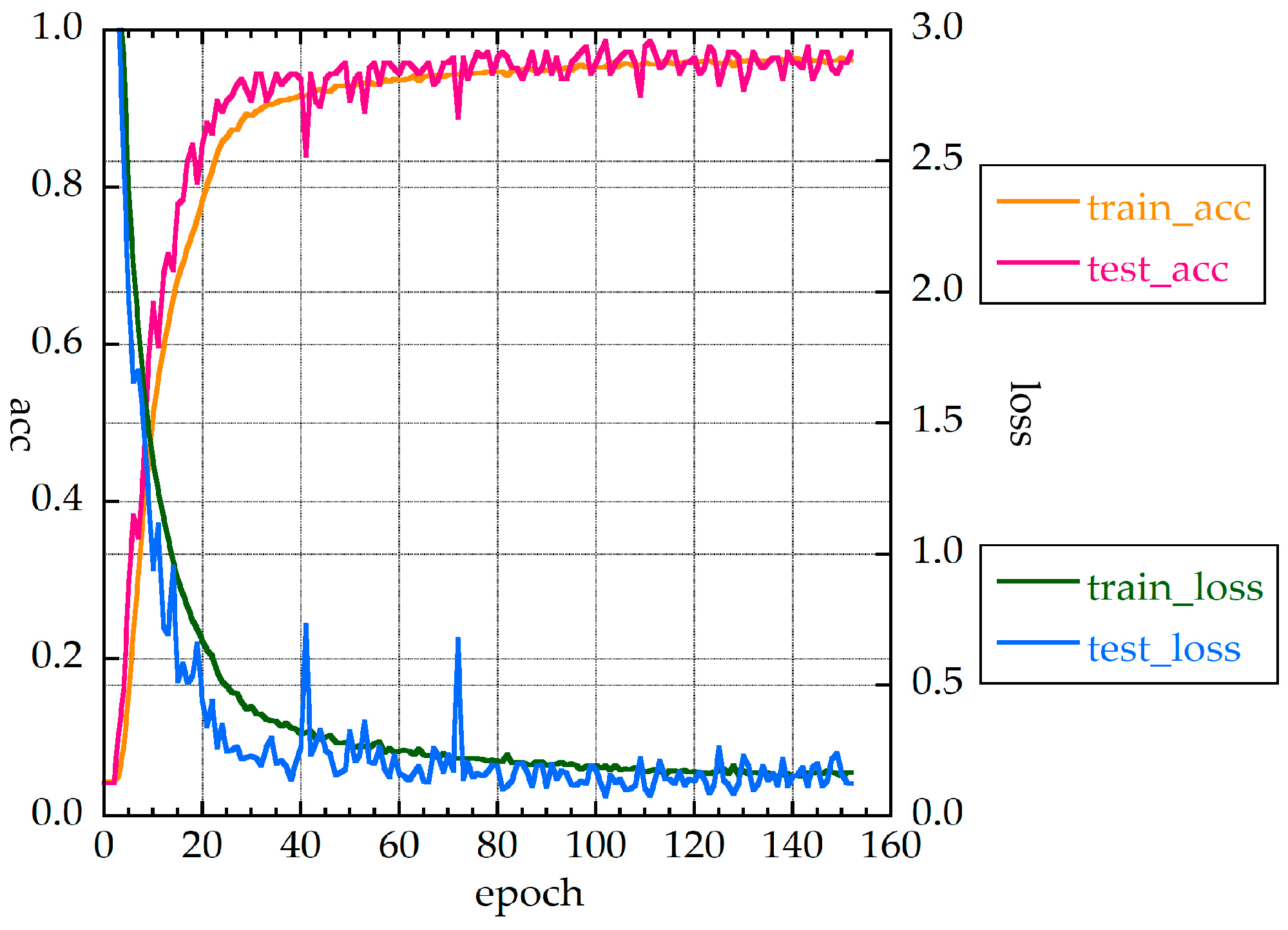
Figure 4 shows the accuracies and loss function values for MLP_S. The test_loss function and test accuracy are somewhat unstable (i.e., they fluctuate). The fluctuation of the loss function was not large, and the function was not overfitted. The best test accuracy (acc) rate was 97.1%. The value of the loss function was less than 0.5 when the epoch number was about 12. The f-value for the test data of the cross-validation was 95.3%, and the f-value including augmentation data (all_f) was 93.1%.
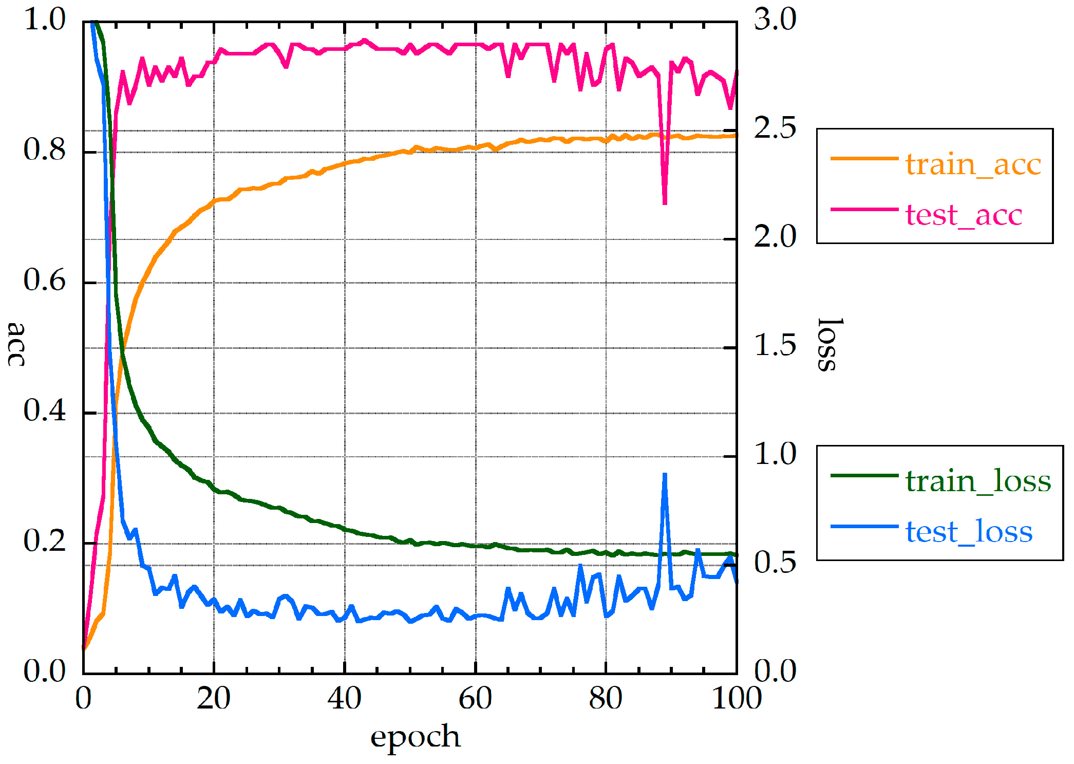
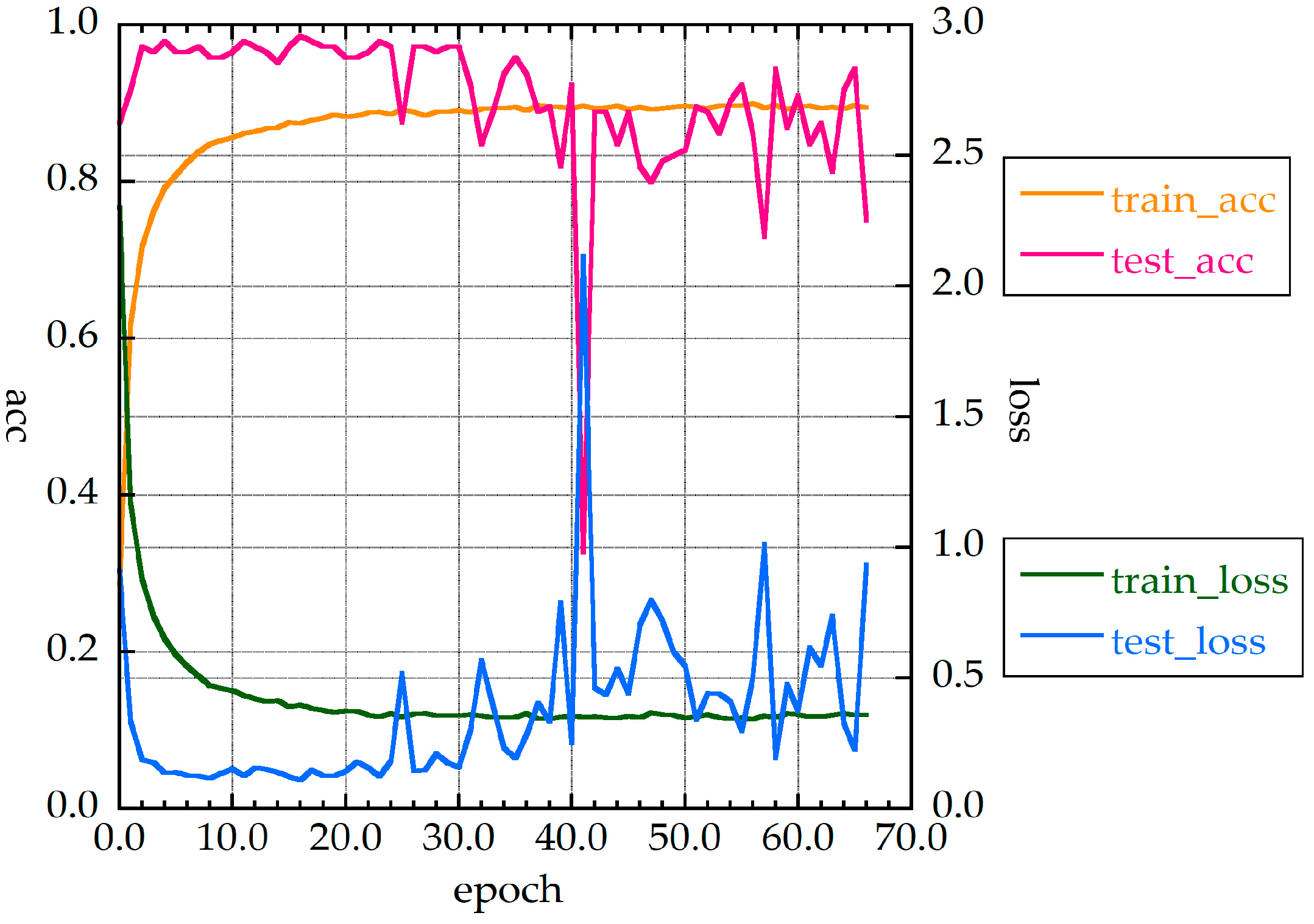
Figure 5 and
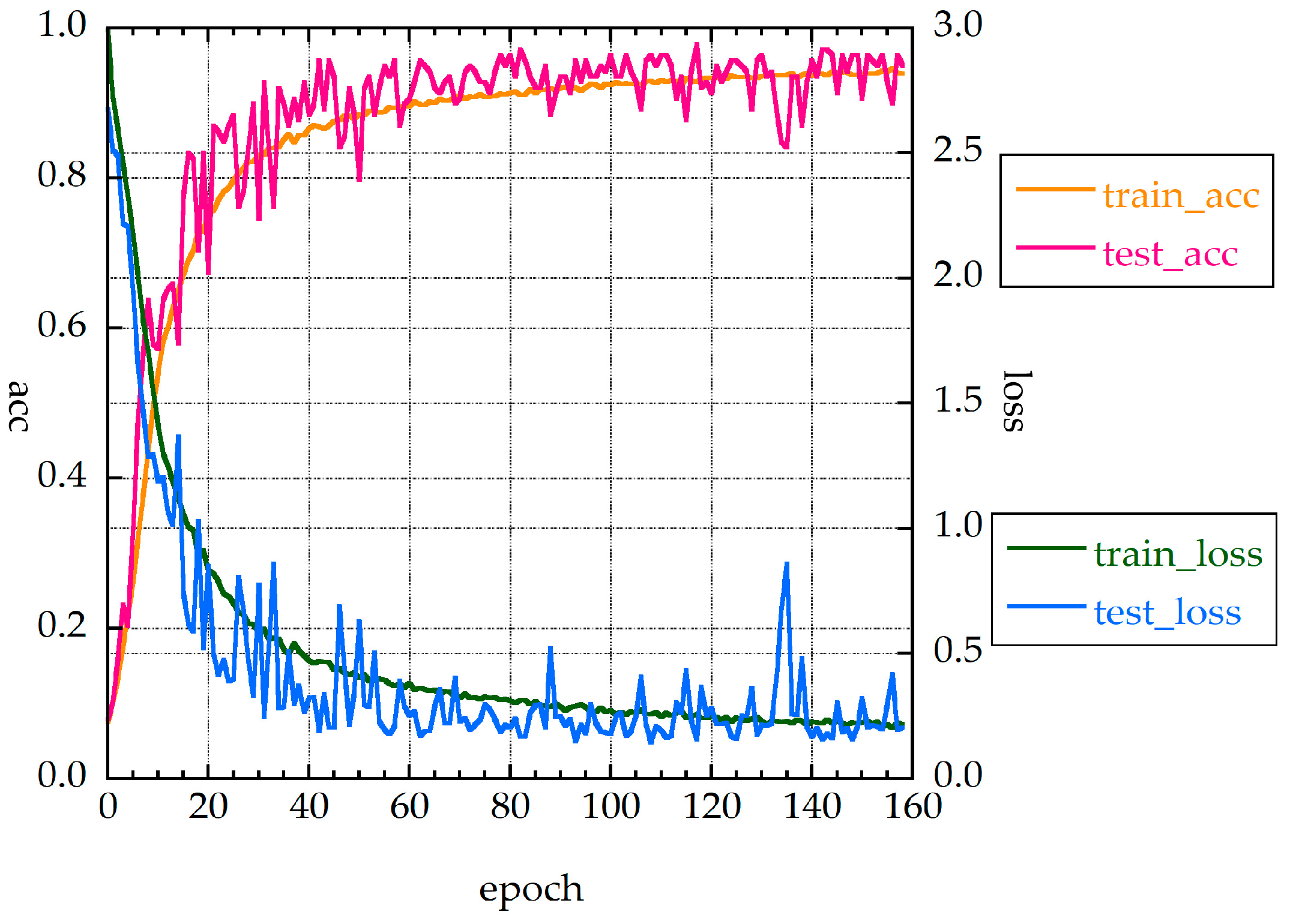
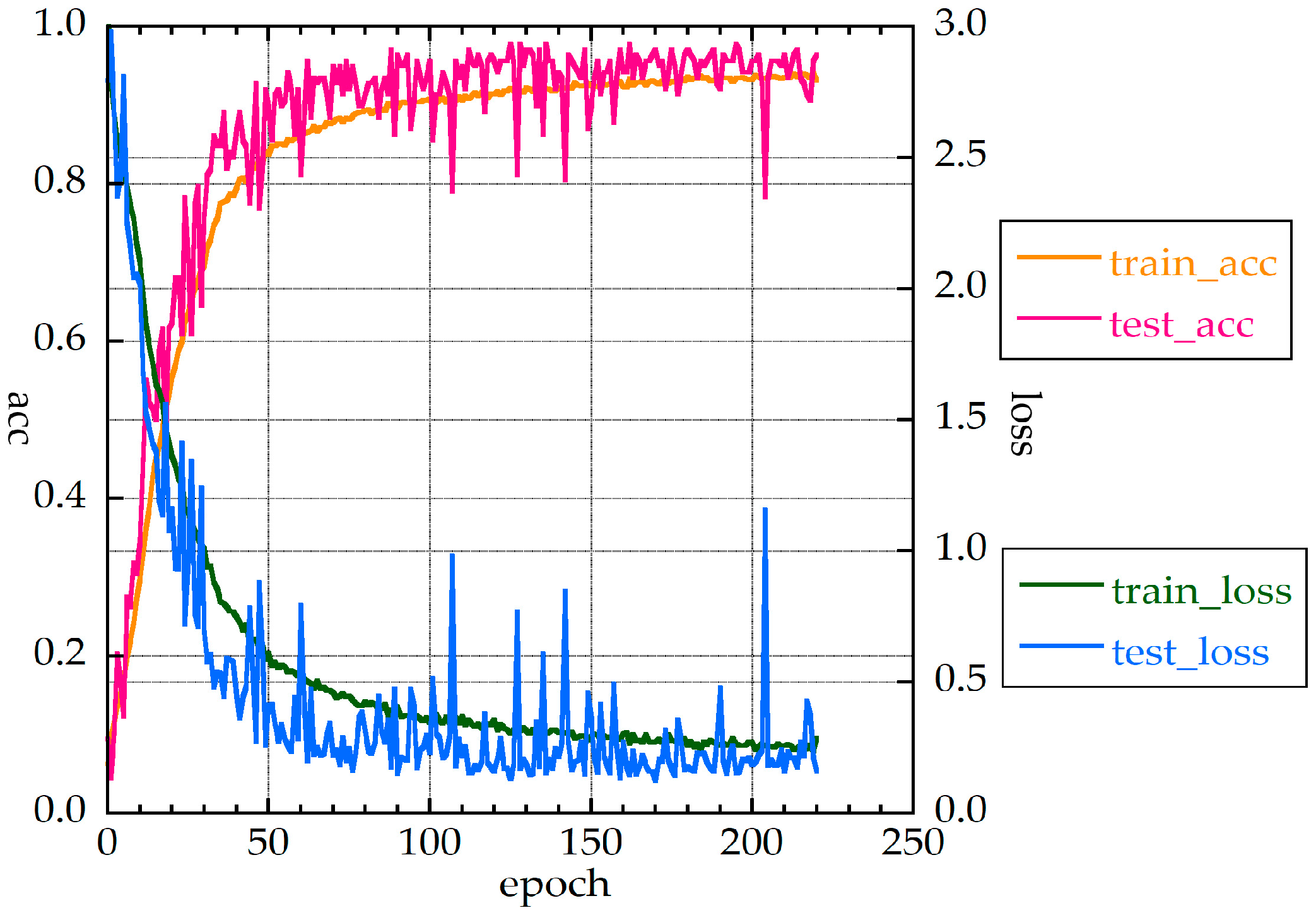
Figure 6 show the accuracies and loss function values for MLP_M and MLP_L, respectively. The loss function values showed large fluctuations. The loss function for MLP_L clearly shows overfitting. As the layer structure became thicker, the loss function tended to exhibit overfitting. The fluctuation of the accuracy rate was large, because the complexity of the problem to be identified did not match the size of the layer structure.
For MLP_M, the accuracy rate was 97.8% for 30 measurements. The value of the loss function was less than 0.5 when the epoch number was about 40. The f- and all_f-values were 95.6% and 93.4%, respectively.
For MLP_L, the fluctuations are larger than those for MLP_M. The value of the loss function was less than 0.5 when the epoch number was over 60, and convergence was slow. The accuracy rate, f-value, and all_f-value were 97.8%, 95.5%, and 92.9%, respectively.
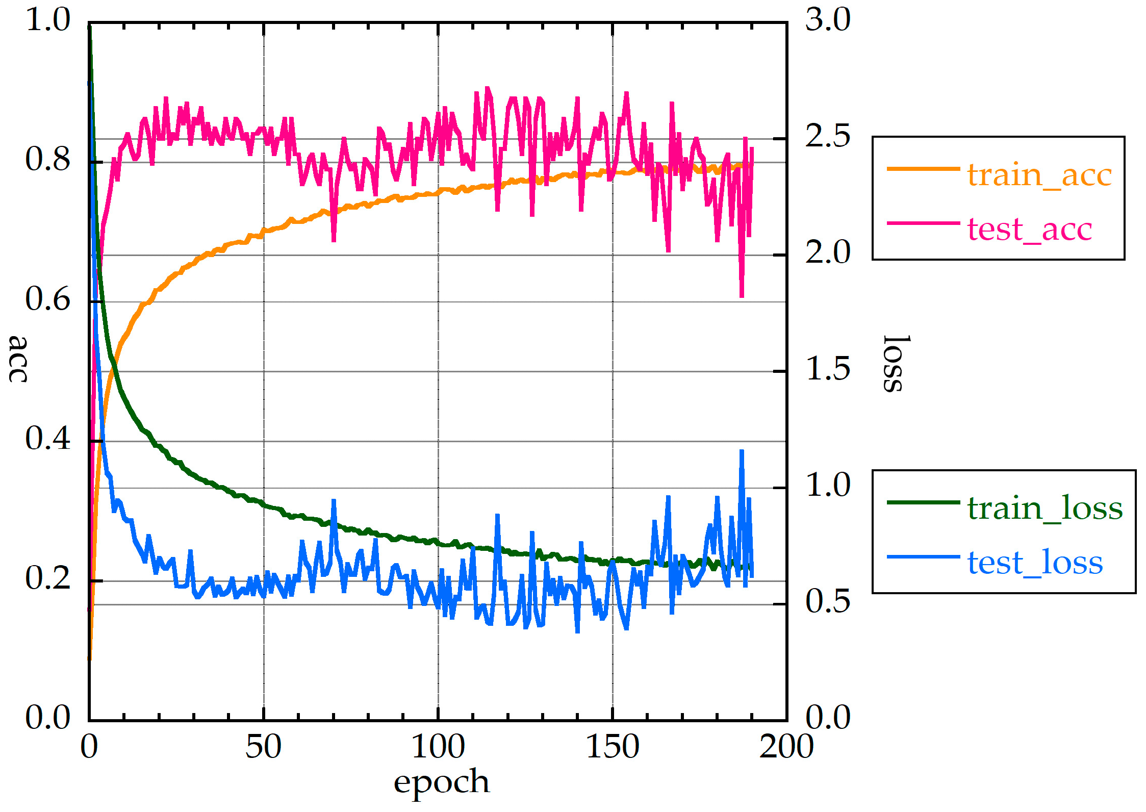
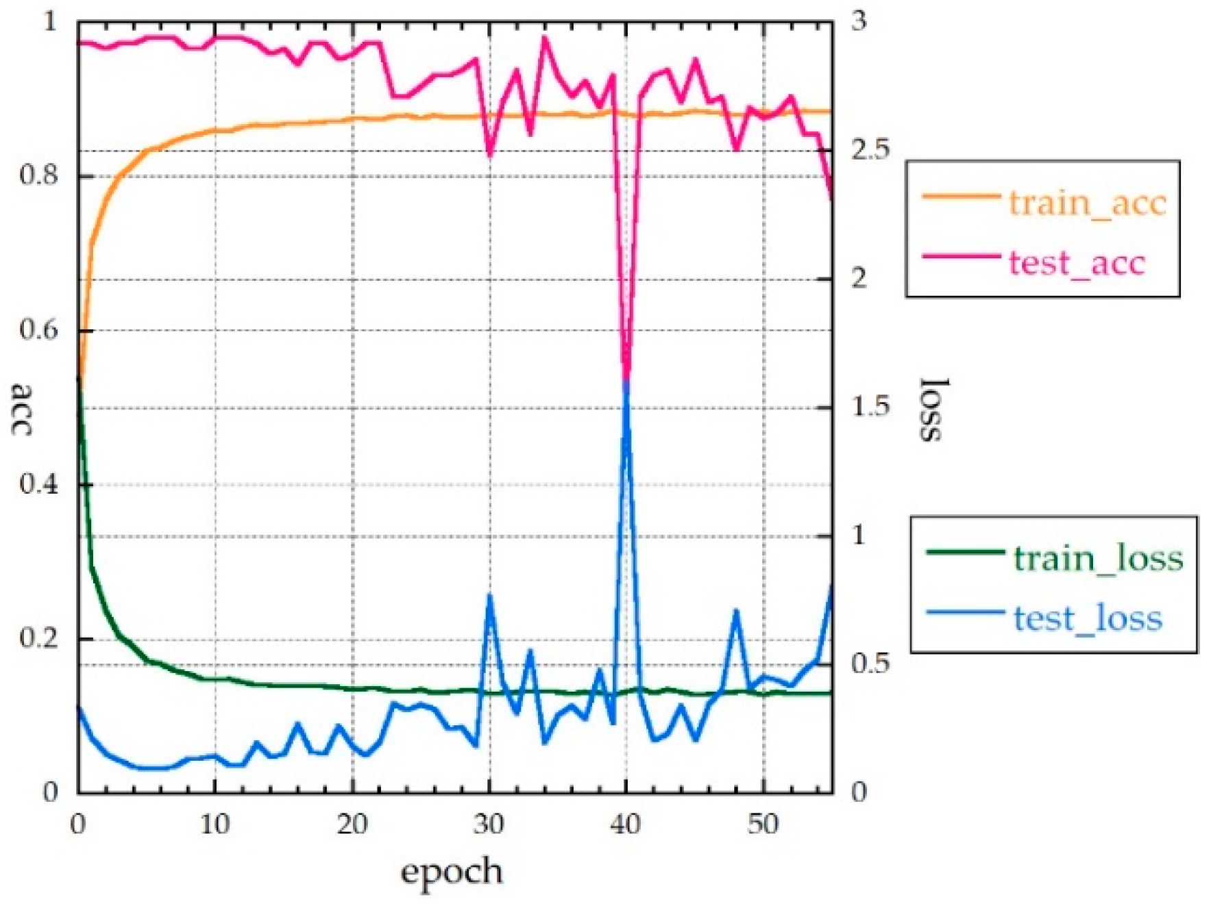
Figure 6 shows accuracies and loss function values for CNN1d.
Table 3 shows the CNN1d structure. The accuracies and loss function values fluctuated, with the loss function exhibiting overfitting. A total of 180 epochs were required for the loss function to be less than 0.5, and convergence was slow. This is a difficult case when determining the system parameters using the early stopping function of Keras. The accuracy rate was 90.6%. The f-value was 88.1%, and the all_f-value was 84.9%. These results indicate that CNN1d is unsuitable for alteration mineral identification. One-dimensional convolution could not learn the form of spectral reflectance, and the max pooling method did not work well. The disturbances in
Figure 7 may be due to the frequent use of dropouts. Additionally, it contained augmentation data when learning, but not when testing. For this reason, test loss was always lower than training loss.
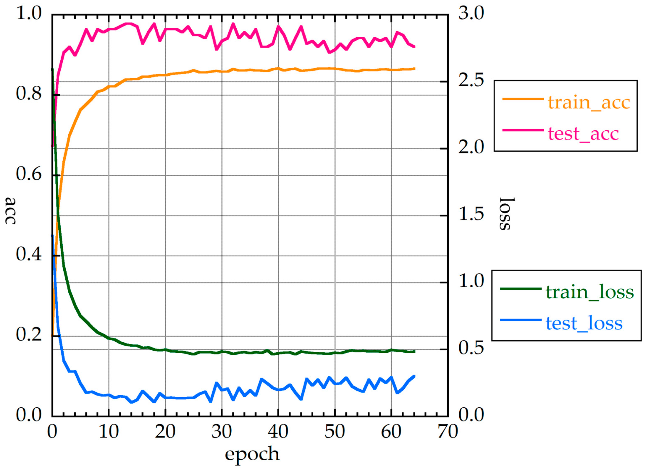
Figure 8 shows the accuracies and loss function values for CNN2d. The original (1773 × 229) image for CNN2d_Hi was compressed to a smaller image (432 × 288). Therefore, the accuracy rate was expected to be low. However, the accuracy rate was equal to or higher than that of the other methods, which indicates that CNN2d is suitable for spectral identification. With CNN2d, learning did not converge, unless some pre-processing was undertaken.
Table 4 shows the layer structure of CNN2d. The number of parameters is small. There are iterations of the convolution layers, max-pooling layers, and drop-out layers. The number of epochs required for the loss function in learning to be less than 0.5 was only 20. Its learning was, thus, fast.
When deciding which algorithm to use, we chose that with a large f-value. If K-fold cross-validation is implemented, the f-value should be used as the representative value of the system.
Table 5 and
Figure 9 show that accuracy increased with the number of measurements of a sample. The differences in the accuracy rates and f-values between NN are small, except CNN1d. However, the graphs of accuracies and loss function values sometimes indicated overfitting, and it is necessary to judge with the graphs.
MLP_S is considered to be the best, based on the f-value without HQ and in terms of the speed of actual learning and overfitting. CNN2d showed good values but required many hours for learning.
Table 5 shows the accuracy of each NN.
Table 6 shows the f-value of K-fold cross-validation without HQ.
Table 7 shows the epoch number required for the loss function to be less than 0.5.
4.2. Deep Learning with HQ
The parameter for augmentation was Aug_type 2 (see
Section 2.2). The identified minerals were from 24 mineral species. The layer structure was the same as that without HQ.
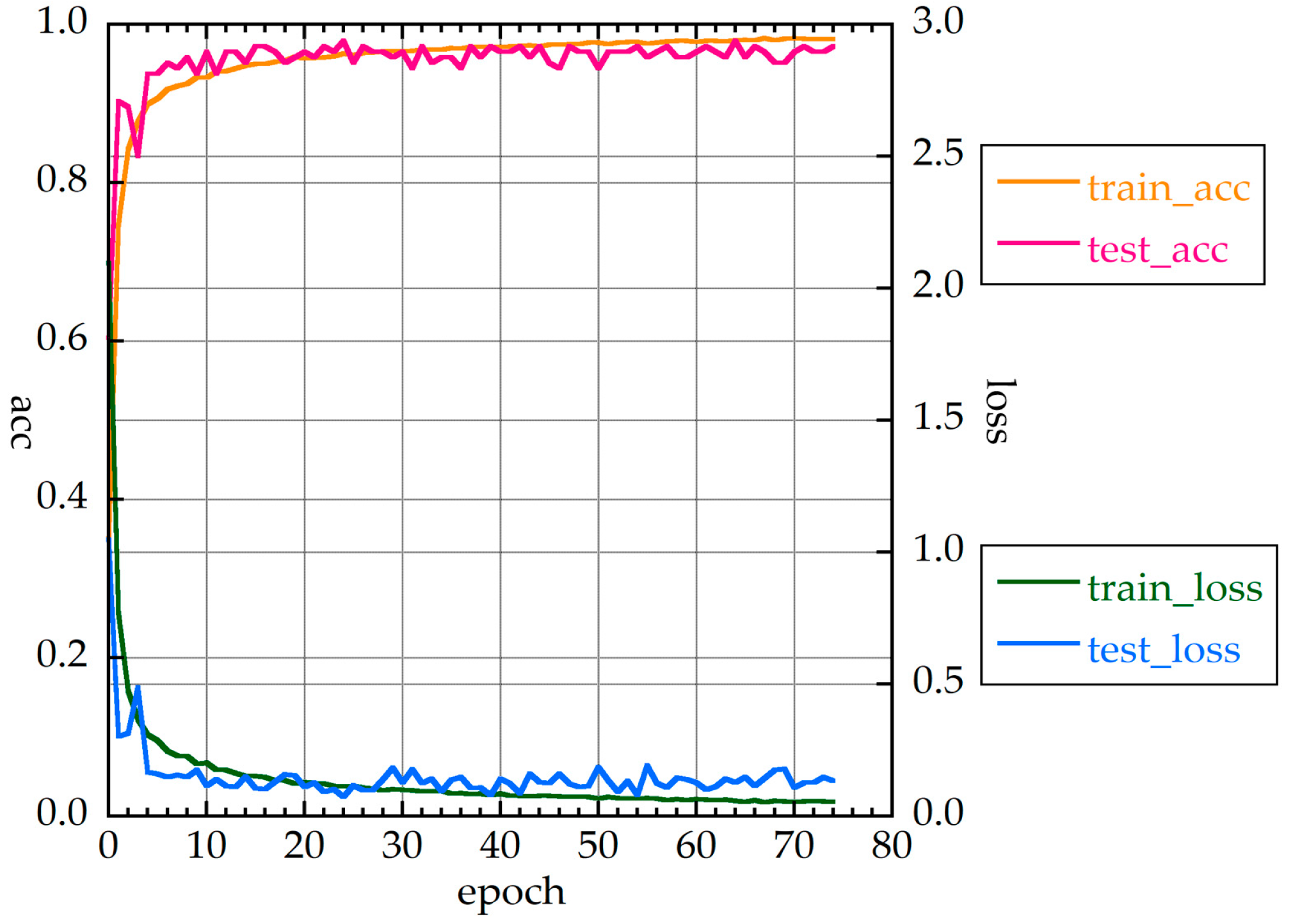
Figure 10 shows the accuracies and loss function values for MLP_S. It can be seen that MLP_S converges quickly, and accuracy is relatively stable.
Figure 11 shows the confusion matrix for MLP_S with HQ for 30 measurements. The values on the diagonal are large, and thus the classification is good. The f-value of MLP_S was high, at 97.1%.
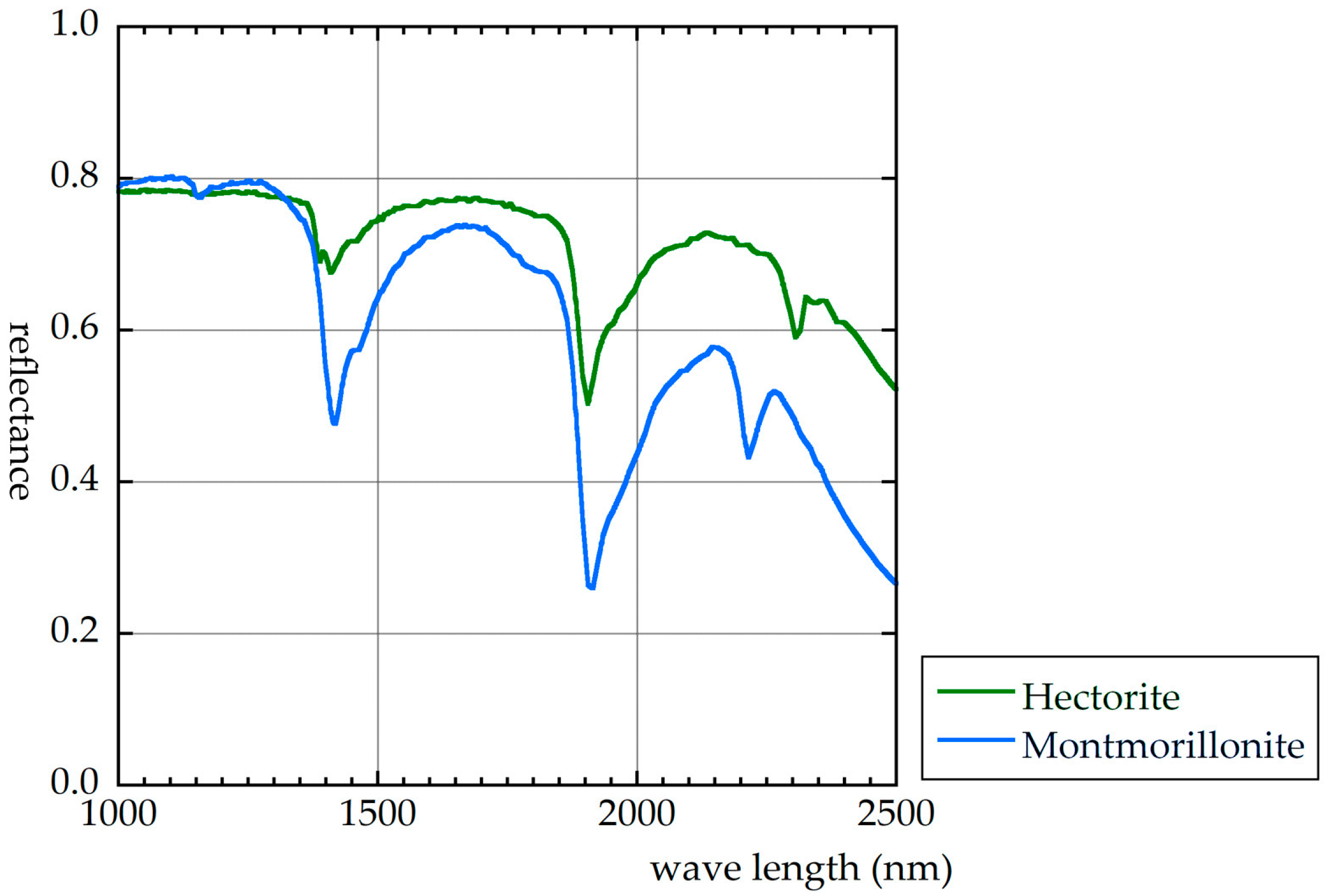
Figure 12 shows the reflectance spectra of hectorite and montmorillonite. An error example is shown in this figure. The distinction between hectorite and montmorillonite was poor. The shapes of the two reflectance spectra are similar; however, the location of absorption is different. DL does not perform identification only by the wavelength position of the absorption. DL is identified using elements of the whole form of the spectral reflectance.
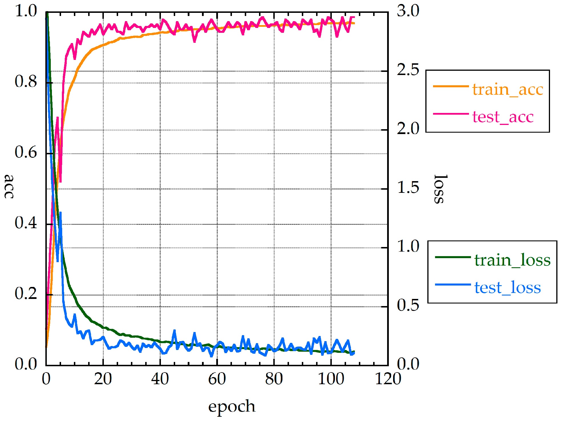
Figure 13 shows the accuracies and loss function values of MLP_M. The figure shows that the tendency for overfitting was very weak for MLP_M.
Figure 14 shows the accuracies and loss function values for MLP_L. The tendency for overfitting was a little strong.
Figure 15 shows the accuracies and loss function values for CNN1d. There was a tendency for overfitting when the epoch number exceeded 90.
Figure 16 and
Figure 17 show the accuracies and loss function values for CNN2d and CNN2d_Hi. Respectively, similar trends can be seen. Distinctive fluctuations appear at 40 epochs. The best-precision values are high, but an appropriate model could not be created without the early stopping function in Keras, before 40 epochs.
Table 8 shows the best test accuracy for each NN. The accuracies were high for all NNs.
Table 9 shows the results of K-fold cross-validation with HQ. Every NN showed a high f-value.
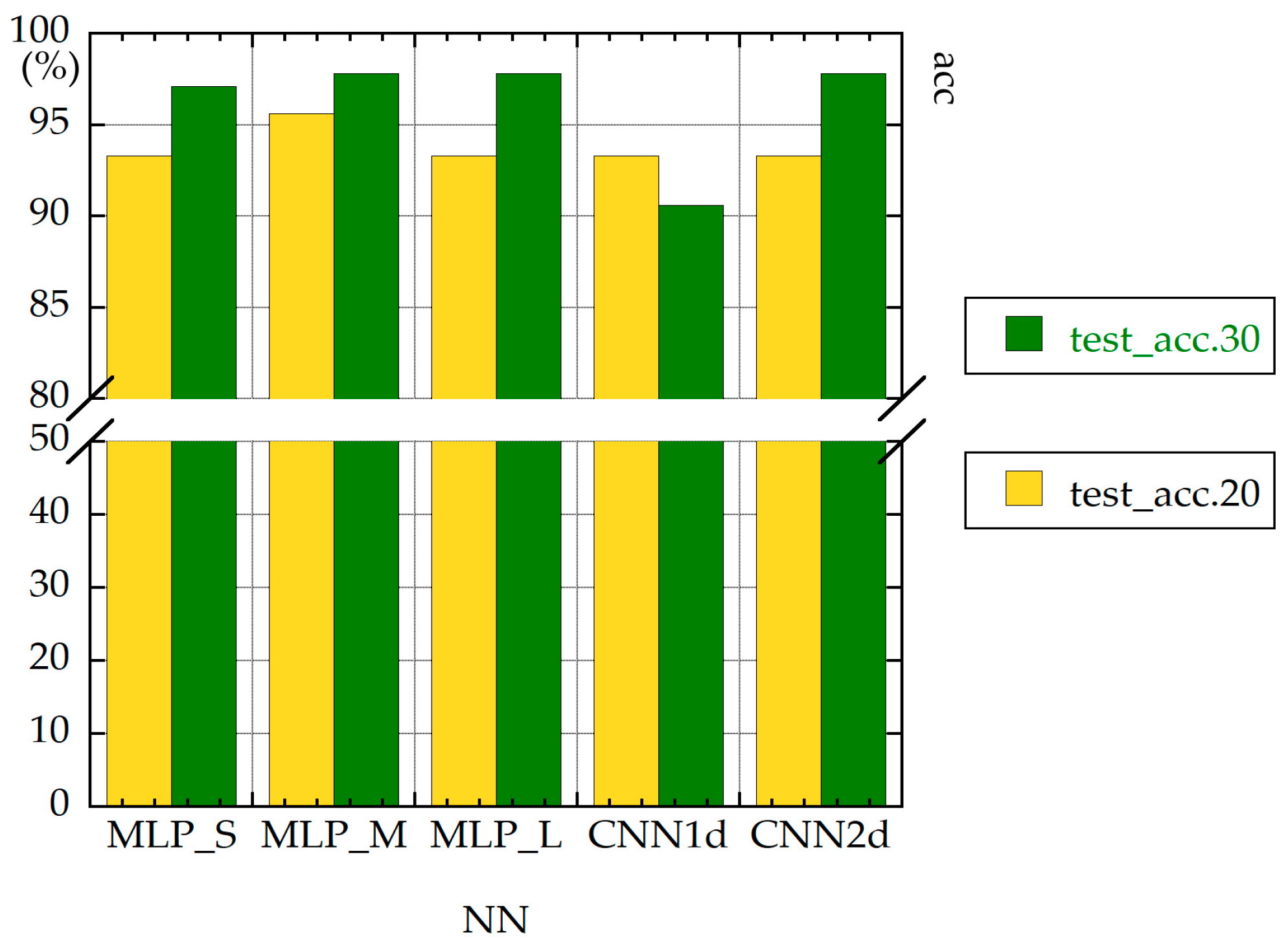
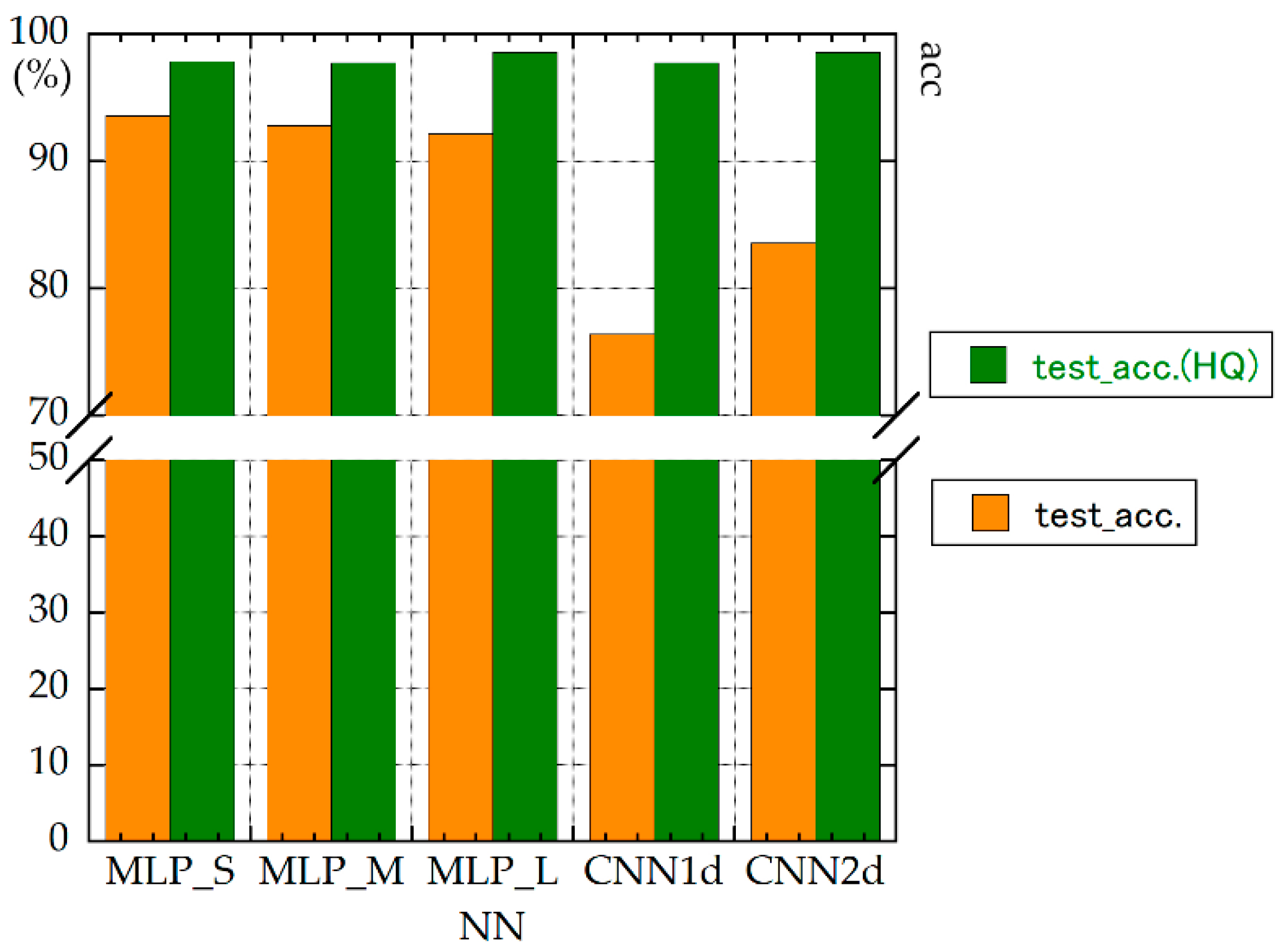
Figure 18 shows that the values of test_acc obtained with HQ were higher than those obtained without HQ.
All NNs had high f-values. For accuracies and loss function values, MLP_S_HQ and MLP_M_HQ quickly converged. These values were high in general
5. Discussion
We applied MLP and CNN to identify alteration minerals. We adjusted the number of layers in an MLP and used one- and two-dimensional CNN. Additionally, a comparison was made between processing with and without HQ.
MLP and CNN both showed high accuracies. HQ improved accuracy. DL using HQ processing showed a value of 97.8% or more for the test accuracy rate and 96.9% or more for the f-value in K-fold cross-validation. This result indicates that it is possible to use empirical knowledge, which is difficult to describe logically on a computer, for mineral identification. This result also indicates that DL found a pattern in the data and extracted feature quantities. In conventional methods, this extraction is done by researchers.
It was found that mineral identification can be done using MLP, even with few layers. Although CNN2d converged quickly and produced a smooth curve, it requires a considerable amount of time for learning, and it is not as quick as MLP in practice.
Although we obtained high accuracy rates using data with HQ processing, extreme caution is required when using augmentation, as noise may be identified as an absorption peak. Before HQ processing, a dataset comprising augmentation data was created based on the signal-to-noise (S/N) ratio of the spectrometer data. However, HQ processing can emphasize noise. Very high accuracies were obtained after we reduced the S/N ratio of the augmentation data by about half.
For the identification of 24 species of alteration minerals, MLP_S_HQ and MLP_M_HQ had high f-values and did not exhibit overfitting. We also obtained a high accuracy rate as measured by the K-fold cross-validation method, as well as others. K-fold cross-validation verified the generalizability of the training data.
Many of the networks tested in this study showed a cross-validation f-value of 97% or more. In addition to accuracy, it is important to consider convergence and overfitting by examining the accuracy and loss function value curves for each model.
The accuracy of CNN1d tended to decrease with the number of measurements of a mineral. This is also shown in the results of K-fold cross-validation. CNN1d showed a low classification accuracy (test_acc = 90.6%); the max pooling layer could not recognize the shape of reflectance spectra. CNN2d showed a high accuracy rate for spectra reduced to 432 × 288. The successful identification, using a coarse-resolution image, shows that CNN2d recognized not only the position of absorption but also the entire shape. The accuracy of the CNN2d_HQ_Hi image was satisfactory. However, the training time required for CNN is much higher than that for MLP_S. In this study, many of the hyperparameters, including the learning rate, were chosen by using the Keras defaults. Adadelta was selected as a learning hyperparameter.
6. Conclusions
This study applied two DL methods, namely MLP and CNN, without and with HQ, to the identification of alteration minerals. The results show that MLP_S_HQ and MLP_M_HQ were the best methods (test_acc > 97.8%), in terms of classification accuracy and overfitting in the identification of 24 alteration minerals. DL can overcome the problem of wavelength shift, despite the noise in the wavelength direction.
MLP_S_HQ exhibited no tendency for overfitting and achieved a high accuracy rate and a high f-value. The DL algorithm extracted the features of reflectance spectra without user intervention. Overfitting was found when the MLP layer structure became thick.
In addition to accuracy, it is important to consider convergence and overfitting by examining the accuracy and loss function value curves for each model; even if the loss value or accuracy is high, if there is a tendency for overfitting, the model must be carefully applied.
We found that HQ processing increases accuracy. HQ is a prominent technique in DL. However, it is important to use some augmentation processing with caution. There are cases where strong noise is recognized as an absorption peak.
DL requires a tremendous amount of time for preparation, including data management, which differs for each DL method. To minimize errors, it is important to determine which DL methodology is the most suitable for solving the target problem. Future research will focus on reducing overfitting, increasing the number of mineral species, and implementing the proposed model on the computer equipped with a spectrometer.
Author Contributions
Conceptualization, Methodology, and Writing, S.T. and Y.Y.; Data curation, S.T.; Programming, S.T., H.T., and K.S.; Funding Acquisition, Y.Y.
Funding
This work was funded by Japan Oil, Gas and Metals National Corporation (JOGMEC) and JSPS KAKENHI (grant no. 15H04225).
Acknowledgments
We would like to express our gratitude to Shuho Noda, Yukie Asano, Yuu Kawakami, and Kazuo Masuda of JOGMEC for their valuable comments regarding the spectral measurements of minerals. We are also grateful to Sinzi Huzikawa of Geotechnos Co., Ltd. and Keisuke Nishi of Deep Ocean Resources Development Co., Ltd. for their constructive discussions.
Conflicts of Interest
The authors declare no conflict of interest.
References
- Ishikawa, Y.; Sawaguchi, T.; Iwaya, S.; Horiuchi, M. Delineation of Prospecting Targets for Kuroko Deposits Based on Modes of Volcanism of Underlying Dacite and Alteration Haloes. Min. Geol. 1976, 26, 105–117. [Google Scholar] [CrossRef]
- Ossandón, C.G.; Fréraut, C.R.; Gustafson, L.B.; Lindsay, D.D.; Zentilli, M. Geology of the Chuquicamata mine A progress report. Econ. Geol. 2001, 96, 249–270. [Google Scholar] [CrossRef]
- Metal Mining Agency of Japan. Development of Simple Identification Technology for Alteration Mineral; Mineral Resource Exploration Technology Development Report; MMAJ: Tokyo, Japan, 1989; p. 393. [Google Scholar]
- Tanabe, K.; Uesaka, H.; Inoue, T.; Takahashi, H.; Tanaka, S. Identification of mineral components from near-infrared spectra by a neural network. Bunseki Kagaku 1994, 43, 765–769. [Google Scholar] [CrossRef]
- Montero, S.; Irene, C.; Brimhall, G.H. Semi-automated Mineral Identification Algorithm for Ultraviolet, Visible and Near-Infrared Reflectance Spectroscopy. In Proceedings of the 6th Annual Conference of the International Association for Mathematical Geology, Cancum, Mexico, 6–12 September 2001. [Google Scholar]
- Kruse, F.A.; Boardman, J.W.; Lefkoff, A.B.; Heidebrecht, K.B.; Shapiro, A.T.; Barloon, P.J.; Goetz, A.F.H. The Spectral Image Processing System (SIPS)—Interactive Visualization and Analysis of Imaging Spectrometer Data. Remote Sens. Environ. 1993, 44, 145–163. [Google Scholar] [CrossRef]
- Ishikawa, S.T.; Gulick, V.C. An Automated Classification of Mineral Spectra. In Proceedings of the 44th Lunar and Planetary Science Conference, Woodlands, TX, USA, 18–22 March 2013. [Google Scholar]
- Liu, J.; Osadchy, M.; Ashton, L.; Foster, M.; Solomone, C.J.; Gibson, S.J. Deep convolutional neural networks for Raman spectrum recognition: A unified solution. Analyst 2017, 142, 4067–4074. [Google Scholar] [CrossRef] [PubMed]
- Boser, B.E.; Guyon, I.M.; Vapnik, V.N. A training algorithm for optimal margin classifiers. In Proceedings of the Fifth Annual Workshop on Computational Learning Theory, Pittsburgh, PA, USA, 27–29 July 1992; pp. 144–152. [Google Scholar]
- Clark, R.N.; Swayze, G.A.; Wise, R.; Livo, E.; Hoefen, T.; Kokaly, R.; Sutley, S.J. USGS Digital Spectral Library splib06a: U.S. Geological Survey Digital Data Series 231. 2007. Available online: https://speclab.cr.usgs.gov/spectral.lib06/ds231/index.html (accessed on 25 April 2019).
- Urai, M.; Sato, I.; Ninomiya, Y.; Kouda, R.; Miyazaki, Y.; Yamaguchi, Y. Reflection Spectrum Catalog of Rocks and Minerals from Visible to Short Wavelength Infrared Region National Institute of Advanced Industrial Science and Technology; Geology Survey Japan Report; Geology Survey of Japan: Tsukuba, Japan, 1989; pp. 129–135. [Google Scholar]
- Banno, Y.; Kouda, R. High-Resolution Reflectance Data of Minerals Deposited in the Geological Museum; The National Institute of Advanced Industrial Science and Technology Geology Survey of Japan Open File Report; Geology Survey of Japan: Tsukuba, Japan, 2014. [Google Scholar]
- Rosenblatt, F. The Perceptron: A Probabilistic Model for Information Storage and Organization in the Brain. Psychol. Rev. 1958, 65, 386–408. [Google Scholar] [CrossRef] [PubMed]
- Rumelhart, D.E.; Hinton, G.E.; Williams, R.J. Learning representations by back-propagating errors. Nature 1986, 323, 533–536. [Google Scholar] [CrossRef]
- Goodfellow, I.; Bengio, Y.; Courville, A. Deep Learning; MIT press: Cambridge, MA, USA, 2016; p. 775. [Google Scholar]
- Silver, D.; van Hasselt, H.; Hessel, M.; Schaul, T.; Guez, A.; Harley, T.; Dulac-Arnold, G.; Reichert, D.; Rabinowitz, N.; Barreto, A.; et al. The predictron: End-to-end learning and planning. In Proceedings of the 34th International Conference on Machine Learning, Sydney, Australia, 6–11 August 2017; pp. 3191–3199. [Google Scholar]
- Zhou, Z.H.; Feng, J. Deep forest: Towards an alternative to deep neural networks. In Proceedings of the Twenty-Sixth International Joint Conference on Artificial Intelligence, Melbourne, Australia, 19–25 August 2017; pp. 19–25. [Google Scholar]
- Lawrence, S.; Giles, C.L.; Tsoi, A.C. Lessons in neural network training: Overfitting may be harder than expected. In Proceedings of the Fourteenth National Conference on Artificial Intelligence, Menlo Park, CA, USA, 27–31 July 1997; pp. 540–545. [Google Scholar]
Figure 1.
Reflectance spectra of alunite without and with hull quotient (HQ).
Figure 1.
Reflectance spectra of alunite without and with hull quotient (HQ).
Figure 2.
Flowchart of the study.
Figure 2.
Flowchart of the study.
Figure 3.
Evaluation methods for deep learning.
Figure 3.
Evaluation methods for deep learning.
Figure 4.
Accuracies and loss function values of MLP_S for 30 measurements without HQ.
Figure 4.
Accuracies and loss function values of MLP_S for 30 measurements without HQ.
Figure 5.
Accuracies and loss function values of MLP_M for 30 measurements without HQ.
Figure 5.
Accuracies and loss function values of MLP_M for 30 measurements without HQ.
Figure 6.
Accuracies and loss function values of MLP_L for 30 measurements without HQ.
Figure 6.
Accuracies and loss function values of MLP_L for 30 measurements without HQ.
Figure 7.
Accuracies and loss function values of CNN1d for 30 measurements without HQ.
Figure 7.
Accuracies and loss function values of CNN1d for 30 measurements without HQ.
Figure 8.
Accuracies and loss function values of CNN2d for 30 measurements.
Figure 8.
Accuracies and loss function values of CNN2d for 30 measurements.
Figure 9.
Test accuracies (20 versus 30 measurements).
Figure 9.
Test accuracies (20 versus 30 measurements).
Figure 10.
Accuracies and loss function values of MLP_S with HQ (MLP_S_HQ).
Figure 10.
Accuracies and loss function values of MLP_S with HQ (MLP_S_HQ).
Figure 11.
Confusion matrix for MLP_S with HQ for 30 measurements.
Figure 11.
Confusion matrix for MLP_S with HQ for 30 measurements.
Figure 12.
Spectral reflectances of hectorite and montmorillonite.
Figure 12.
Spectral reflectances of hectorite and montmorillonite.
Figure 13.
Accuracies and loss function values of MLP_M_HQ.
Figure 13.
Accuracies and loss function values of MLP_M_HQ.
Figure 14.
Accuracies and loss function values of MLP_L_HQ.
Figure 14.
Accuracies and loss function values of MLP_L_HQ.
Figure 15.
Accuracies and loss function values of CNN1d_HQ.
Figure 15.
Accuracies and loss function values of CNN1d_HQ.
Figure 16.
Accuracies and loss function values of CNN2d_HQ.
Figure 16.
Accuracies and loss function values of CNN2d_HQ.
Figure 17.
Accuracies and loss function values of CNN2d_Hi_HQ.
Figure 17.
Accuracies and loss function values of CNN2d_Hi_HQ.
Figure 18.
Test accuracies (without HQ versus with HQ).
Figure 18.
Test accuracies (without HQ versus with HQ).
Table 1.
List of target alteration minerals.
Table 1.
List of target alteration minerals.
| | Mineral Name | Type | Alteration | Temperature | Remark |
|---|
| 1 | alunite | hydrothermal | acidic | low-high | |
| 2 | anhydrite | hydrothermal | acidic | high | propylite |
| 3 | calcite | hydrothermal | intermediate | medium-high | |
| 4 | chlorite | hydrothermal | intermediate | high | propylite |
| 5 | dickite | hydrothermal | acidic | medium-high | pyrophyllite |
| 6 | dolomite | skarmization | - | - | |
| 7 | epidote | hydrothermal | intermediate | high | propylite |
| 8 | gibbsite | bauxite | - | - | |
| 9 | goethite | hydrothermal | gossan | - | |
| 10 | gypsum | hydrothermal | kuroko | - | |
| 11 | halloysite | hydrothermal | acidic | low | |
| 12 | hectorite | lithium | - | - | |
| 13 | illite | hydrothermal | intermediate | medium-high | |
| 14 | jarosite | hydrothermal | - | low | |
| 15 | kaolinite | hydrothermal | acidic | medium | |
| 16 | montmorillonite | hydrothermal | intermediate | low | |
| 17 | muscovite | hydrothermal | intermediate | | |
| 18 | natrolite | hydrothermal | alkali | medium | |
| 19 | nontronite | hydrothermal | basic | low | |
| 20 | phlogopite | hydrothermal | - | - | skarmization |
| 21 | pyrophyllite | hydrothermal | acidic | high | |
| 22 | rhodochrosite | hydrothermal | - | - | |
| 23 | talc | hydrothermal | - | - | skarmization |
| 24 | vermiculite | hydrothermal | - | - | granite |
Table 2.
The layer structure of MLP_S.
Table 2.
The layer structure of MLP_S.
| Layer Type | Output | Parameter# |
|---|
| dense_1 | (None, 512) | 871,424 |
| dropout_1 | (None, 512) | 0 |
| dense_2 | (None, 512) | 262,656 |
| dropout_2 | (None, 512) | 0 |
| dense_3 | (None, 256) | 131,328 |
| dropout_3 | (None, 256) | 0 |
| dense_4 | (None, 23) | 5912 |
Table 3.
The layer structure of CNN1d for 30 measurements.
Table 3.
The layer structure of CNN1d for 30 measurements.
| Layer Type | Output | Parameter# |
|---|
| conv2d_1 | (None, 1, 1599, 32) | 128 |
| max_pooling2d_1 | (None, 1, 799, 32) | 0 |
| dropout_1 | (None, 1, 799, 32) | 0 |
| conv2d_2 | (None, 1, 797, 64) | 6208 |
| max_pooling2d_2 | (None, 1, 398, 64) | 0 |
| dropout_2 | (None, 1, 398, 64) | 0 |
| conv2d_3 | (None, 1, 396, 128) | 24,704 |
| max_pooling2d_3 | (None, 1, 198, 128) | 0 |
| dropout_3 | (None, 1, 198, 128) | 0 |
| flatten_1 | (None, 25344) | 0 |
| dense_1 | (None, 64) | 1,622,080 |
| dropout_4 | (None, 64) | 0 |
| dense_2 | (None, 32) | 2080 |
| dropout_5 | (None, 32) | 0 |
| dense_3 | (None, 23) | 759 |
Table 4.
The layer structure of CNN2d for 30 measurements.
Table 4.
The layer structure of CNN2d for 30 measurements.
| Layer Type | Output | Parameter# |
|---|
| conv2d_1 | (None, 286, 430, 32) | 896 |
| max_pooling2d_1 | (None, 95, 143, 32) | 0 |
| dropout_1 | (None, 95, 143, 32) | 0 |
| conv2d_2 | (None, 93, 141, 64) | 18496 |
| max_pooling2d_2 | (None, 31, 47, 64) | 0 |
| dropout_2 | (None, 31, 47, 64) | 0 |
| conv2d_3 | (None, 29, 45, 128) | 73856 |
| max_pooling2d_3 | (None, 9, 15, 128) | 0 |
| dropout_3 | (None, 9, 15, 128) | 0 |
| conv2d_4 | (None, 7, 13, 128) | 147584 |
| max_pooling2d_4 | (None, 2, 4, 128) | 0 |
| dropout_4 | (None, 2, 4, 128) | 0 |
| flatten_1 | (None, 1024) | 0 |
| dense_1 | (None, 64) | 65600 |
| dropout_5 | (None, 64) | 0 |
| dense_2 | (None, 32) | 2080 |
| dropout_6 | (None, 32) | 0 |
| dense_3 | (None, 23) | 759 |
Table 5.
Accuracy of each neural network (NN) (best test_acc value).
Table 5.
Accuracy of each neural network (NN) (best test_acc value).
| Number of Measurements | Mineral Species | Epoch | Type of Layer | Train_Accuracy | Test_Accuracy |
|---|
| | | 19 | MLP_S | 91.1 | 93.3 |
| | | 73 | MLP_M | 94.5 | 95.6 |
| 20 times | 9 | 77 | MLP_L | 94.2 | 93.3 |
| | | 13 | CNN1d | 78.3 | 93.3 |
| | | 79 | CNN2d | 97.6 | 93.3 |
| | | 67 | MLP_S | 93.6 | 97.1 |
| | | 117 | MLP_M | 92.8 | 97.8 |
| 30 times | 23 | 125 | MLP_L | 92.2 | 97.8 |
| | | 114 | CNN1d | 76.4 | 90.6 |
| | | 13 | CNN2d | 83.6 | 97.8 |
Table 6.
Results of K-fold cross-validation without HQ.
Table 6.
Results of K-fold cross-validation without HQ.
| Network | Accuracy | Precision | Recall | f | all_acc | all_pr | all_rc | all_f |
|---|
| MLP-S | 95.2 | 96.0 | 95.2 | 95.3 | 93.1 | 93.7 | 93.1 | 93.1 |
| MLP-M | 95.7 | 96.1 | 95.7 | 95.6 | 93.4 | 93.8 | 93.4 | 93.4 |
| MLP-L | 95.5 | 96.1 | 95.5 | 95.5 | 92.9 | 93.4 | 92.9 | 92.9 |
| CNN1D | 87.8 | 90.6 | 87.8 | 88.1 | 84.3 | 87.9 | 84.3 | 84.9 |
| CNN2D | 95.4 | 96.0 | 95.4 | 95.4 | 93.2 | 93.9 | 93.2 | 93.3 |
Table 7.
Epoch number required for loss function to be less than 0.5.
Table 7.
Epoch number required for loss function to be less than 0.5.
| DL Type | Number of Epoch |
|---|
| MLP_S | 12 |
| MLP_M | 40 |
| MLP_L | 60 |
| CNN1d | >180 |
| CNN2d | 20 |
Table 8.
Accuracy of each NN (best test_acc) with HQ.
Table 8.
Accuracy of each NN (best test_acc) with HQ.
| Number of Measurements | Mineral Species | Epoch | Type of Layer | Accuracy | Test_Accuracy |
|---|
| | | 24 | MLP_S | 96.3 | 97.9 |
| | | 117 | MLP_M | 92.8 | 97.8 |
| 30 times | 24 | 102 | MLP_L | 95.4 | 98.6 |
| | | 13 | CNN1d | 83.9 | 97.8 |
| | | 16 | CNN2d | 87.5 | 98.6 |
| | | 4 | CNN2d_Hi | 80.9 | 98.6 |
Table 9.
Results of K-fold cross-validation with HQ.
Table 9.
Results of K-fold cross-validation with HQ.
| Network | Accuracy | Precision | Recall | f | all_acc | all_pr | all_rc | all_f |
|---|
| MLP_S | 97.1 | 97.4 | 97.1 | 97.1 | 95.8 | 96.0 | 95.8 | 95.8 |
| MLP_M | 96.9 | 97.3 | 96.9 | 96.9 | 95.8 | 96.0 | 95.8 | 95.7 |
| MLP_L | 97.1 | 97.5 | 97.1 | 97.1 | 95.5 | 95.7 | 95.5 | 95.5 |
| CNN1d | 95.0 | 95.1 | 95.0 | 94.8 | 93.8 | 94.2 | 93.8 | 93.7 |
| CNN2d | 96.9 | 97.3 | 96.9 | 97.0 | 96.0 | 96.3 | 96.0 | 96.0 |
| CNN2d_Hi | 97.1 | 97.6 | 97.1 | 97.1 | 96.4 | 96.7 | 96.4 | 96.4 |
© 2019 by the authors. Licensee MDPI, Basel, Switzerland. This article is an open access article distributed under the terms and conditions of the Creative Commons Attribution (CC BY) license (http://creativecommons.org/licenses/by/4.0/).


