Measurement of In-Situ Flow Rate in Borehole by Heat Pulse Flowmeter: Field-Case Study and Reflection

Abstract

Large-scale groundwater flow modelling demands comprehensive geological investigation (GI) to accurately predict groundwater dynamics during open-cut and underground mining. Due to the existence of large-scale heterogeneity (e.g., fault and fracture) in natural geological strata (e.g., overburden soil, rock mass and coal seam), the in-situ flow measurement in boreholes, compared to laboratory seepage tests, can bring more reliable information to estimating the in-situ seepage properties (e.g., hydraulic conductivity, intrinsic permeability, transmissivity and specific yield). In this paper, a flow-measuring technique-heat pulse flowmeter (HPFM) is methodologically introduced and then practically applied for GI in the mining extension zone of Hunter Valley Operations (HVO), New South Wales, Australia. The measuring experiences, including both positive and negative outcomes, are reported and discussed with a series of datasets of in-situ flow rates measured in the selected boreholes. The pros and cons of the HPFM application in HVO are also discussed and summarised based on the user experience collected through this field trip. Finally, through a thorough reflection, some practical recommendations are provided to help other HPFM practitioners bypass all difficulties experienced on this trip. It is anticipated that valuable user information can contribute to better GI in other sites when performing this measuring technique.

1. Introduction

1.1. Project Engineering Background

As Australia became the top-ranking coal explorer and consumer, almost 85% of Australian electricity production relies on coal-burning fire power stations [1]. In principle, there are two main mining methods: open-cut and underground. The open-cutting mining method has been increasingly used in Australia, requiring excavating the overburdened soil and rock strata before mining. After unloading the overburdened geological strata above the coal seam layer, groundwater drainage from the ambient geoenvironmental system (e.g., the adjacent aquifer and river) will further exacerbate the surface water and groundwater-dependent ecosystem [2]. With an aim to appropriately assess and manage such risks, the novel in-situ geological investigation (GI) methods have been encouraged to conduct before the open-cut mining operation [3,4,5,6].

1.2. Review of Multi-Scale Groundwater Theories

Since groundwater and vadose zone modelling were developed based on linear and non-linear diffusion theories, the modelling accuracy is highly dependent on the determination of the diffusion coefficient (i.e., diffusivity (D)), which can be given by the hydraulic conductivity (k) (i.e., coefficient of permeability in geomechanics and geotechnical engineering) divided by the specific storage (S_s) (i.e., the storage coefficient, equivalent to the storativity (S) for the general groundwater equation in diffusion form) [7,8,9,10,11,12]. To further simplify the groundwater modelling at a large scale, the Boussinesq equation was further developed under the Dupuit assumption that the horizontal scale is much over the vertical scale of groundwater table variation [7,11,12]. With such a modelling simplification, the in-situ k measurement for confined/unconfined aquifers can be replaced by the determination of in-situ transmissivity (T = kB or T = kH), which is equal to the in-situ k multiplied by the thickness (B) of a confined aquifer or the total hydraulic head (H) of an unconfined aquifer, where fractures and faults embed [7]. In addition, the storativity under the Dupuit assumption should be given as S = S_y + S_sB for an aquifer including both unconfined and confined in thickness B (S_y is the specific yield for the unconfined aquifer, and S_s is the specific storage for the confined aquifer) [11,12].

1.3. Review of Shortages of Laboratory Seepage Tests

Usually, the seepage measurement could be conducted in the laboratory based on seepage testing standards [13,14,15] or innovative testing platforms [16] with novel sensor techniques [17]. Those standard and novel seepage tests have also been combined with computational fluid dynamic (CFD) models to better understand seepage mechanics at the pore scale [18,19,20,21]. Nonetheless, those laboratory-scale seepage characterisations were only applicable to a natural or artificial porous medium at representative elementary volume (REV) scale under the assumption of isotropic and homogenous conditions [22,23]. Also, those testing methods will not function properly for the in-situ measurement of seepage properties, i.e., hydraulic properties for groundwater systems (e.g., k, S_y, S_s and T) due to their scale limitations and the presence of large-scale heterogeneity (e.g., fault, fracture, joint, coal cleat, etc.) [24,25,26,27], possibly forming the preferential paths of seepage flow [28,29]. In comparison to the laboratory-measured k and intrinsic permeability (K) (where K = μk/ρg, and μ, ρ and g are borehole fluid-dynamic viscosity, density and gravitational acceleration, respectively) for an intact geomaterial (e.g., intact rock and coal specimens), such pre-existed geological structure, mainly the fracture and fault networks in the underground rock mass and coal seam [25], could yield much higher k or K in several orders of magnitude [30]. In addition, the in-situ stress condition also governs the values of seepage properties (e.g., k, K, S_s, T and S) by mechanically dominating the orientation, spacing, aperture size, length, etc. of fractures and faults in their networks [24,31,32], so the laboratory determination of relatively intact geomaterial under much lower stress conditions (i.e., without high in-situ stress from overburden strata) will definitely cause the failure of large-scale groundwater modelling, thereby resulting in unreliable risk assessment and management for the surrounding aqueous environment.

1.4. Review of In-Situ Geological Investigation Methods

As failing to estimate the in-situ seepage properties for fracture and fault networks leads to significant underestimation of groundwater discharge and adverse impacts on the ambient ecosystem during the mining operation, novel in-situ GI methods have drawn more attention from both geotechnical engineering and hydrogeological researchers. By far, there have been multiple novel GI methods (i.e., geophysical methods) to characterise the lithological features in confined/unconfined aquifers, such as calliper logging for borehole dimension, temperature logging for the temperature of groundwater in/outflow, borehole water level measurement for hydrostatic pressure, in-situ pressure logging for possible overpressure, density logging for earth pressure and stress distribution, resistivity logging and sonic logging for geological formations as well as an acoustical (or optical) televiewer system for possible fractures and faults detected along borehole walls [5,33].

1.5. Review of In-Situ Flow Measuring Techniques

In addition to those methods, the in-situ measurement of k, K and T could be achieved by conducting slug-tests and pumping tests for single borehole or multiple boreholes in assistance with analytical solutions, such as Theis and Thiem equations [6,34]. Hence, in-situ flow logging has often been adopted to detect flow rates along geological profiles inside boreholes, and groundwater modelling studies have been taking advantage of in-situ flow logging datasets to investigate groundwater contamination issues [35,36,37,38,39,40]. Many flow logging devices, such as the electromagnetic and impeller flowmeter [41], as well as the dilution technique by electrolyte tracing based on electrical conductivity measurement [42], have been implemented at an early stage in the field and henceforth comprehensively reviewed by Monier-Williams et al. [43]. Nevertheless, there is a lower limitation or rather-called lowest threshold of flow rate that can be precisely measured by those conventional techniques (e.g., impeller flowmeter).

1.6. Review of Heat Pulse Flowmeter Development

In order to measure the low flow rates (0.113–3.815 l/min) with an acceptable precision (5–15%), which was undetectable by the conventional impeller flowmeter, the heat pule flowmeter (HPFM) was therefore developed. In fact, the HPFM is not a newly developed technique and has been applied in the field since the middle of the 1980s by Hess [44] and Paillet et al. [45]. The functioning principle is based on tacking temperature changes to indicate the inflow and outflow into a borehole [46]. After a heat grid wire ignites a heat pulse in between two thermistor sensors, the temperature variation during borehole water flowing can be measured by those two sensors; then, the flow rate can be analysed based on the heat pulse logging; as a result, it was named the heat pulse flowmeter. Since the invention of the HPFM, very scarce literature has introduced this flowmeter into in-situ GI by ambient (natural hydraulic gradient-induced) and stressed (injection/pumping) testing conditions [45,47,48,49,50]. By conducting the single borehole test under quasi-steady conditions, the T and H could be effectively estimated by analysing the HPFM signals [49]. After implementing the cross-borehole tests under transient flow conditions, the values of S and S_s, in addition to T and H, could also be determined by the HPFM based on a groundwater inversion modelling technique developed by Paillet [47].

1.7. Research Challenges Identification

Although the HPFM has been continuously developed in the last three decades, this flowmeter has rarely been applied to characterise the large-scale heterogeneity in the field. Compared to exclusively implementing the mature GI methods, incorporating the HPFM into GI cannot only offer an alternative approach to examining the fractures and faults but also bring more physical insights into in-situ flow investigations. Furthermore, with limited experience in using the HPFM in the field, this technique still owns its inherent constraints (e.g., HPFM probe imperfectly fitting into boreholes, the suspension of silty and clayey particles clogging into the probe, thereby covering the sensors, insufficient flow around the thermal sensors, sensors insensitiveness for specific flow rates, easiness of damaging sensors during installation and disassembly, etc.) in dealing with flow measurement in complex geostructures [5,6,50]. Sometimes, the success of large-scale heterogeneity characterisation is more dependent on the experience of signal analysers. Therefore, carrying out in-situ flow tests with the HPFM and sharing the user experience with new datasets could still be a worthful academic pursuit in engineering geology.

1.8. Field Selection and Research Objective

In this paper, the flow-measuring technique-HPFM is first introduced and then practised in the Hunter Valley Operations (HVO) mining extension zone, New South Wales (NSW), Australia. Both positive and negative measuring experiences are reported in detail and then explained with the detected in-situ flow rates for each selected borehole. Next, the advantages and disadvantages of carrying out the HPFM in HVO are discussed in-depth and summarised based on the user experience collected through this field trip. Finally, with a thorough self-reflection, some practical recommendations are provided to orientate other HPFM users to bypass all challenges encountered on this trip. It is expected that valuable user information can facilitate better GI in other sites when the HPFM is performed.

2. Methodology and Field Study

2.1. HPFM Specification and Working Principle

The heat pulse flowmeter (HPFM) is a type of flowmeter developed for detecting low flow rates below the lower flow rate limits that the traditional impeller flowmeter can measure. According to the manual of HFP-2293 [51], manufactured by Mount Sopris Instrument Co., Denver, CO, USA, it is able to determine its general properties and specifications as listed in

Table 1. General properties of the HFP-2293 (Heat pulse flowmeter (HPFM) probe).

Specification	Values
Power requirements	D.C. voltage at probe tip. Min. 30 VDC and Max. 68 VDC @ 200 mA
Tool output	Pulse type, positive going, 1.25 uS wide from 4.5 kHz to 37,000 kHz
Measuring range	0.113 l/min to 3.785 l/min
Resolution	5% (0.1836 l/min)
Accuracy	5% (mid-range) to 15% (extremes) (0.1836–0.5508 l/min)
Dimensions	Length = 122 cm, Diameter = 4.1 cm, Weight = 15.5 kg

.

The HPFM functioning principle is that since a heat grid wire (see Figure 1a) increases the temperature in between two thermistor sensors (see Figure 1a), the temperature variation during borehole water advection and conduction is able to be detected by those two sensors; then, the flow rate can be analysed based on the heat pulse logging by those sensors. Therefore, it was so-defined the heat pulse flowmeter (HPFM) (see Figure 1b).

There are several applications for measuring the flow rate of a vertical borehole flow profile:

• Initially, characterising and delimiting any individual geological units or formations (e.g., fractures and faults) along each borehole profile.
• Then, separating the flow zones based on the characterised geological formations.
• Further estimating the far-field hydraulic head of the aquifer having fractures and faults (H), hydraulic gradients (dH/dz) and transmissivity (T) for those flow zones.
• Subsequentially, identifying any potential flow conduits.
• Consequently, numerical modelling (e.g., forward and inverse modelling) and hydrogeological mapping.

2.2. HPFM In-Situ Installation

In addition, following the manual of HFP-2293 [51], the principles and operation of the HPFM can be summarised below:

(1)

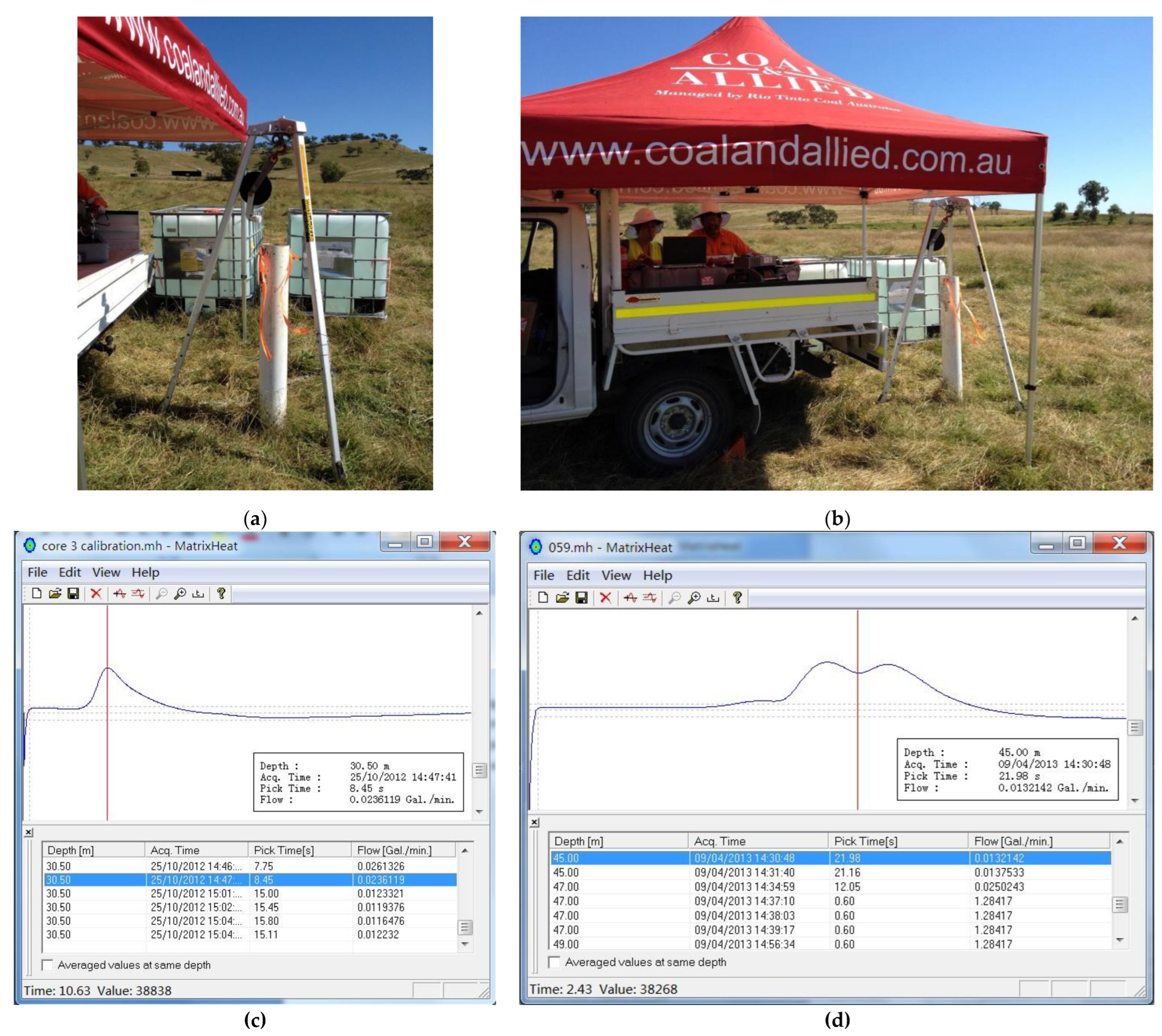
Lower the HPFM probe into each borehole by a cable connected to a winch (see Figure 2a).

(2)

Measure the water flow rate by pressing the trigger assembly button when the probe is centrally positioned at an investigating depth in a borehole.

(3)

The centre conductor of the probe will receive a pulse; then, this pulse will fire the heat grid wire, and the software will receive the signal through the surface monitoring equipment to start a flow measurement (see Figure 2b).

(4)

The heated water transports with the in-situ flow in each borehole from the heat gird wire to the upper or lower thermistor sensor.

(5)

An amplifier will detect the temperature difference between the upper and lower sensors.

(6)

The amplifier’s output will then be converted to a frequency, sent out through the data cable, and finally monitored by the surface equipment and plotted in software (see Figure 2b–d).

(7)

When surface equipment and software have received the information, the tool will charge the capacitors immediately.

(8)

After the capacitors are charged, they will produce the voltage for the heat gird wire to be prepared for the next round of flow rate measurement.

(9)

Finally, the flow rate measurement is completed after the period between raising a heat pulse and the flow-carried peak temperature variation accurately detected by the sensor located above or below the heat grid wire (see Figure 2c,d).

Both the ambient (natural hydraulic gradient-induced) and stressed (injection/pumping) testing conditions must be considered during this measuring process because the data analysis requires different flow rates and hydraulic gradients under various conditions, and both T and far-field H need to be determined through a groundwater inversion modelling process. Therefore, each measurement should be repeated at least three times for each depth of interest. As for the depth selection, undoubtedly, the finer the depth interval, the better the spatial resolution. In fact, such selection depends on various factors, including previously detected geological formations by other GI methods, suspected fracturing or faulting zones, labour/cost-performance trade-offs, etc. Thus, the experienced user can flexibly adjust their depth selection based on their experience and already-known geoinformation, while the new practitioner can try the finer one (e.g., 20–30 cm in this field test) and later increase depth intervals (e.g., 40–50 cm in this field test) accordingly, gaining more experience for each site in the field. After the ambient test has been conducted to measure the flow rate in each borehole, the water injection test should be implemented repeatedly for other flow measurements. The water storage in white colour could supply this water injection, as shown in Figure 2a. Once the tank-stored water is fully drained, if it is necessary, the pumping tests can also be carried out by collecting the pumped water into those tanks. The injection/pumping flow rates can be measured using a manual flowmeter in the in/outlet tube. The steady-state condition could be achieved when the flow rate stabilises over the testing period.

2.3. HPFM Data Analysis

2.3.1. Heat Pulse Signal Processing

When measuring the flow rates of the ambient and stressed tests, the temperature-time plot can be read using the appending software of HFP-2293: MatrixHeat [51]. A typical flow rate display in MatrixHeat is shown in Figure 2c, where the x-axis represents the time, and the y-axis represents the temperature. The measurement is obtained in about 10 s to 45 s. During this period, the software will automatically pick a peak time, which is the time point of the sensor detecting the heat pulse, and the flow rate at this time point can be considered the accurate flow rate at this position.

However, the flow rate display is not always as typical as in Figure 2c. For example, Figure 2d shows a flow rate display that is hard to find out the correct peak point. Under conditions shown in Figure 2d, a series of points can be identified as the peak point. Unfortunately, the software always cannot automatically pick up the correct peak point, so the peak point must be re-picked up by manually adjusting the picking options available in MatrixHeat. If the new peak point still seems unreasonable, such a peak point has to be manually picked up by moving the red line based on user experience. As shown in Figure 2d, where two peaks were encountered, the middle point between the two peaks is highly recommended to be manually selected.

2.3.2. Flow Rate Profile Analysis

After selecting the correct single peak point or middle point between two peaks, the result could be automatically transferred into flow rates by MatrixHeat. Then, it is possible to average flow rates with the same depths in a data spreadsheet; as aforementioned, investigators should take triplicate measurements at each interesting depth. Finally, the data can be displayed as scatter charts (see Figure 3, where the vertical axis shows the borehole depth, and the horizontal axis shows the borehole water flow rates). For the flow measurement in each borehole, the positive values indicate the in-situ flows in the upward direction, while the negative values indicate the in-situ flows in the downward direction. Figure 3 shows a profile of the in-situ flow rates plotted to characterise the inflow and outflow zones corresponding to possibly detected flow-producing geological formations along a borehole profile. For example, the abrupt variation of flow rates could indicate an inflow or outflow between the borehole and the adjacent geological formations.

It should be noted that the scatter chart is a straightforward checking approach that can help judge whether this dataset is valuable or not for any future analysis. The judgment criteria are shown below:

(1)

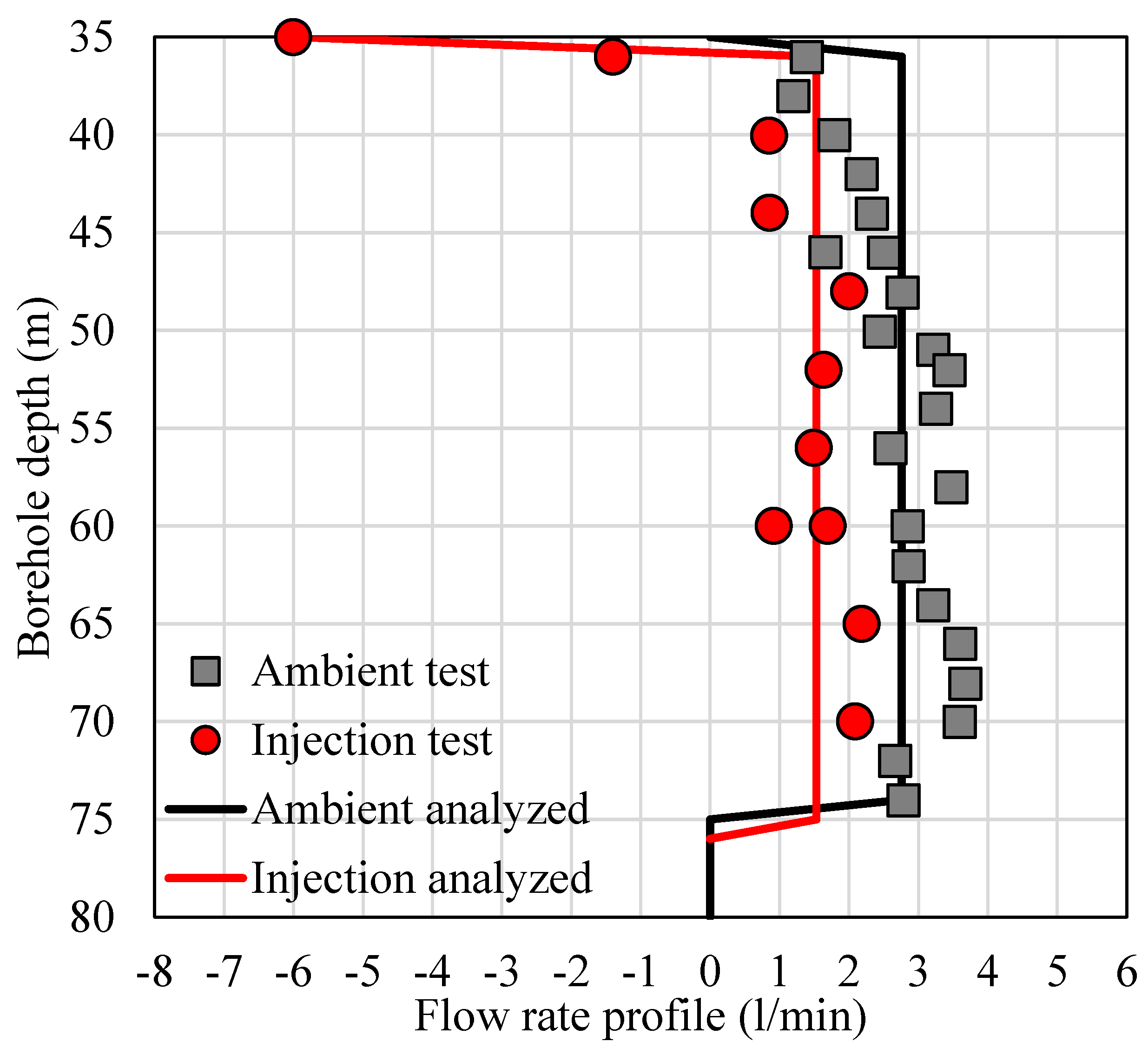
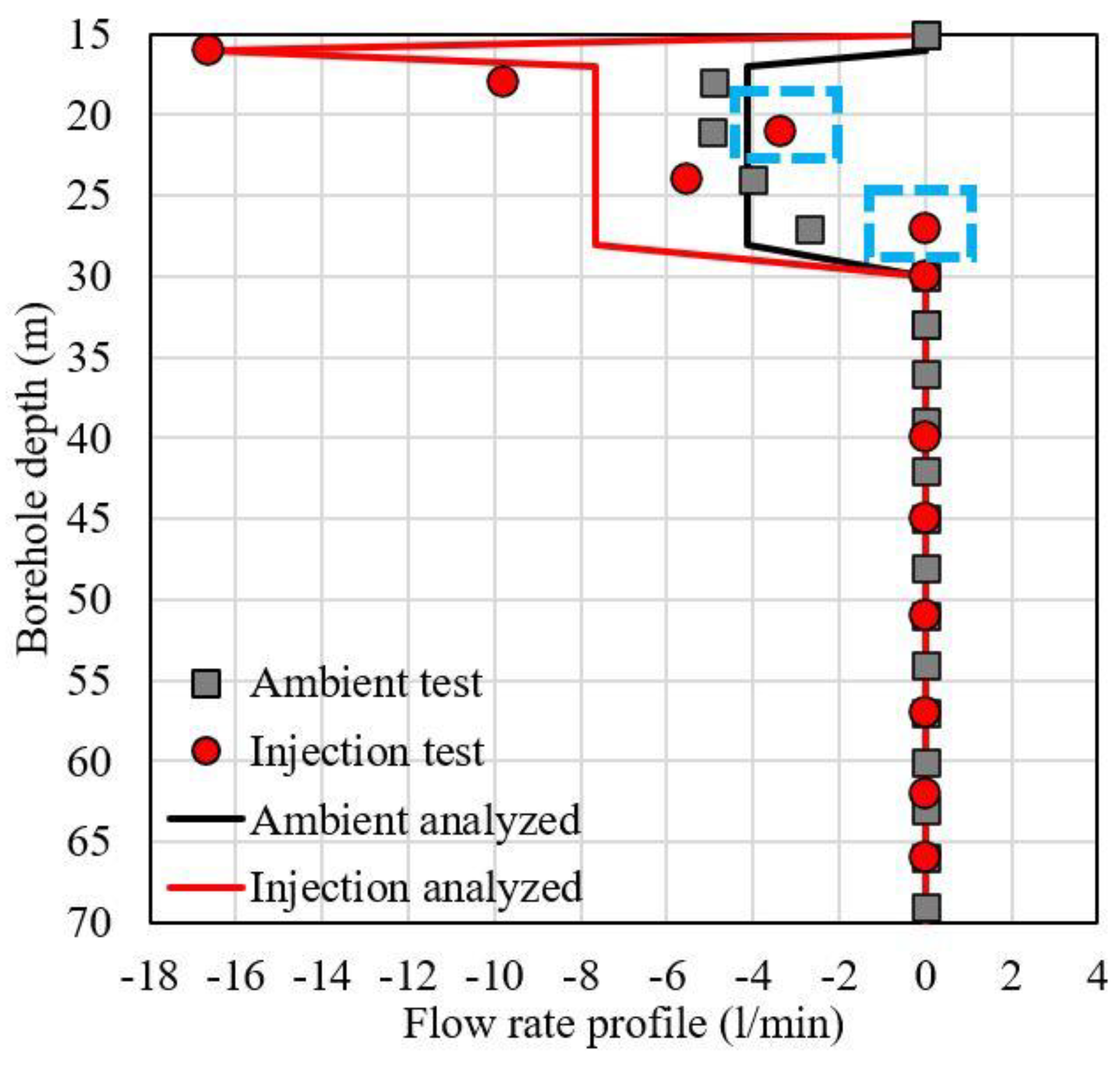
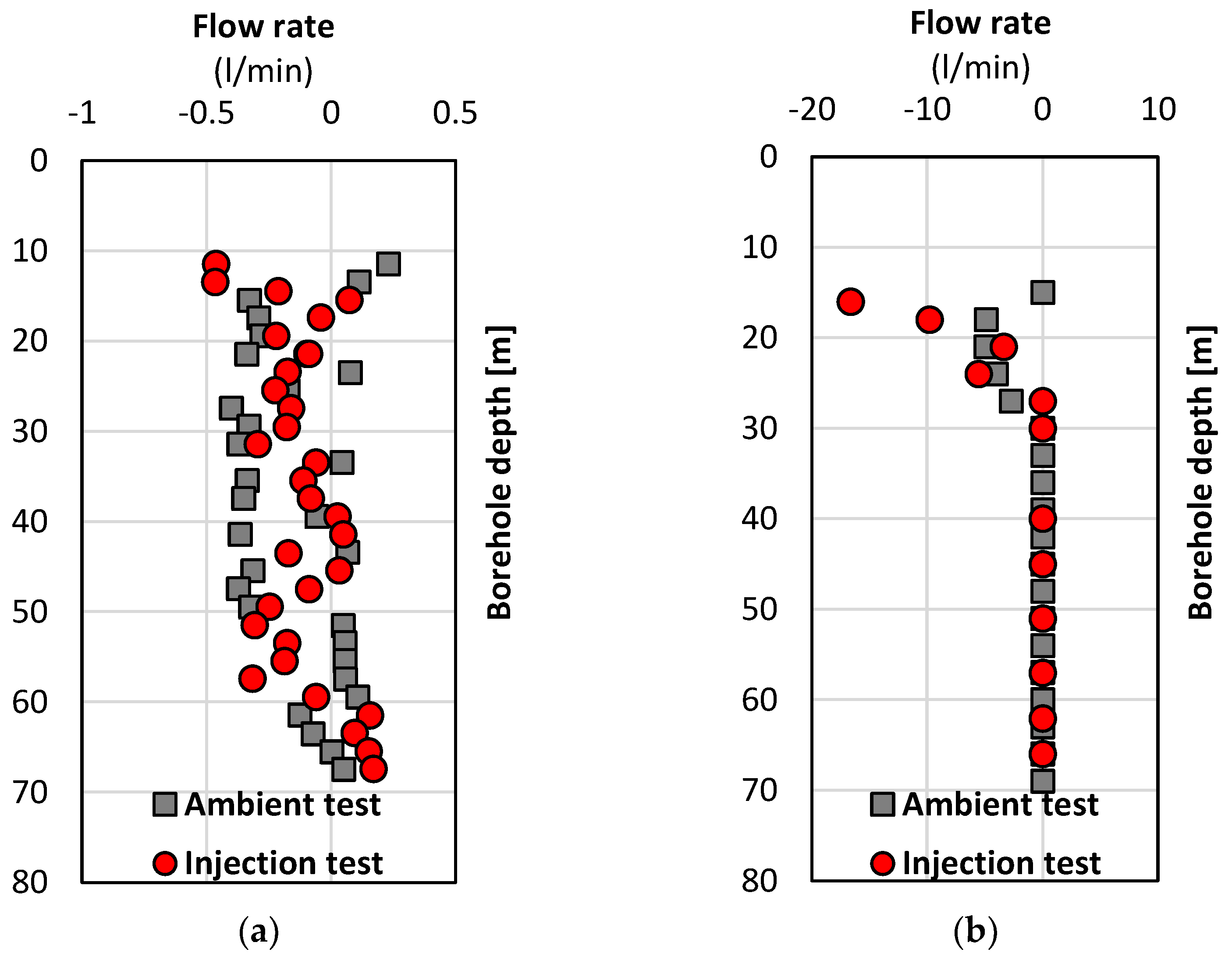
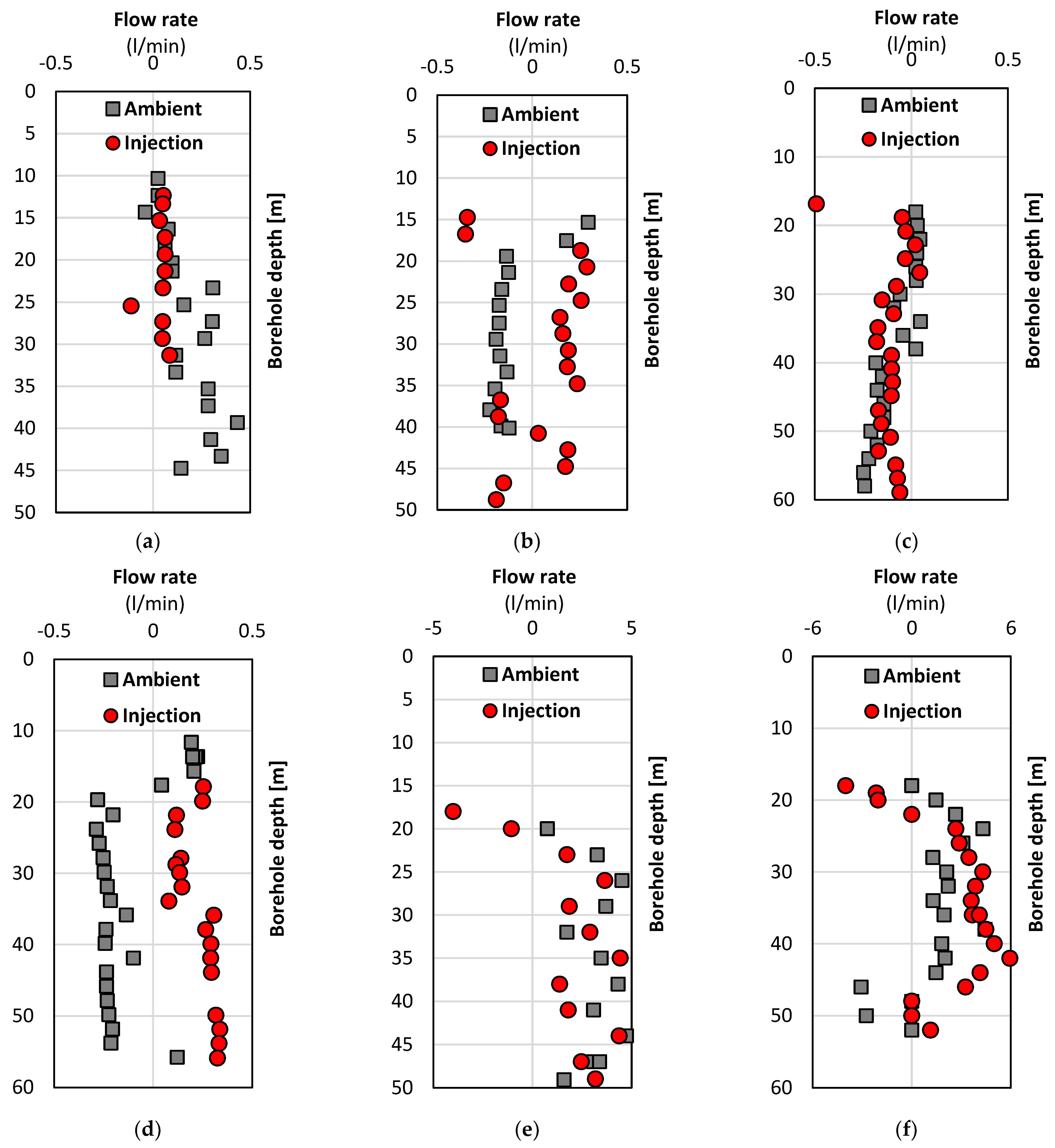
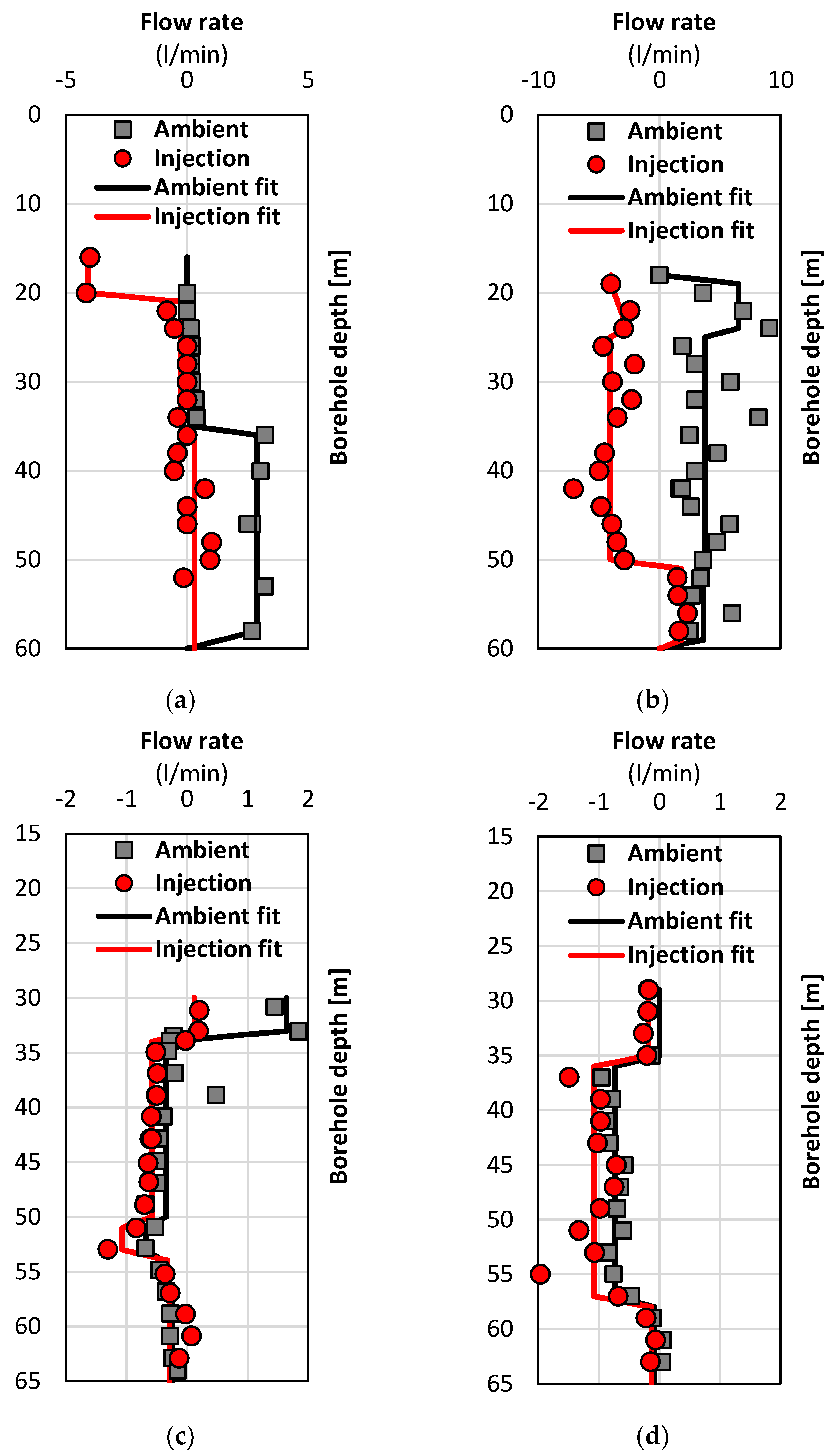
The distribution of the flow rate scatters in standard form but should not be in a littery pattern (mussy, covered with littering and untidy data scatters) compared to successful instances of flow rate profiles in publications.

(2)

The scatter distribution is reasonable, meaning that most data points of the injection test should be on the left side of the datasets of the ambient tests, which is the case in this fieldwork. However, if any HPFM practitioner carried out pumping tests, most data points of the pumping test should be on the right side of the datasets of the ambient tests.

After judging the value of the dataset, if the data is valuable for further analysis, the first step is to estimate the position of a flow-producing zone by the flow rate profile. Specifically, there might be a flow-producing geological formation at any borehole depth when a significant change in flow rates is presented. This geological formation identification could be verified by using the density and calliper loggings to check the accuracy of the formation estimations. Subsequently, the flow rate profile can be separated into zones by the estimated flow-producing zone, followed by adjusting the flow rates by a calibration (the HPFM-detected flow rates to actual flow rates) and calculating the average flow rate for each designated zone. An example of the HPFM output analysis between ambient and pumping tests after formation characterisation is given in

Table 2. An instance of the fracture identification of flow rate profile for borehole A435_R_056.

	Ambient Test				Injection Test
Depth [m]	HPFM [l/min]	Adjusted [l/min]	Zone Average [l/min]	Depth [m]	HPFM [l/min]	Adjusted [l/min]	Zone Average [l/min]
29	NF *	0.00	0.00	30	2.46	2.95	2.91
				31	2.38	2.88
34			Fracture 2
40	−1.14	−1.36	−1.25	35	1.14	1.36	1.44
				40	1.21	1.44
50	−0.98	−1.17		50	1.14	1.36
				55	1.25	1.51
60	−0.98	−1.17		60	1.21	1.44
				70	1.32	1.59
73			Fracture 1
74	NF *	0.00	0.00	74	NF *	0.00	0.00

* NF indicates no flow.

.

The next step is to calculate the subtraction in/outflows based on the principle of mass conservation:

(1)

Calculate the following separately under ambient conditions and injection/pumping conditions:

(a)

Calculate the average water flow rates of each zone (delimited by fractures).

(b)

Calculate the in/outflows of each fracture, which is the difference between the average flow rate above the fracture and the average flow rate below the fracture.

(c)

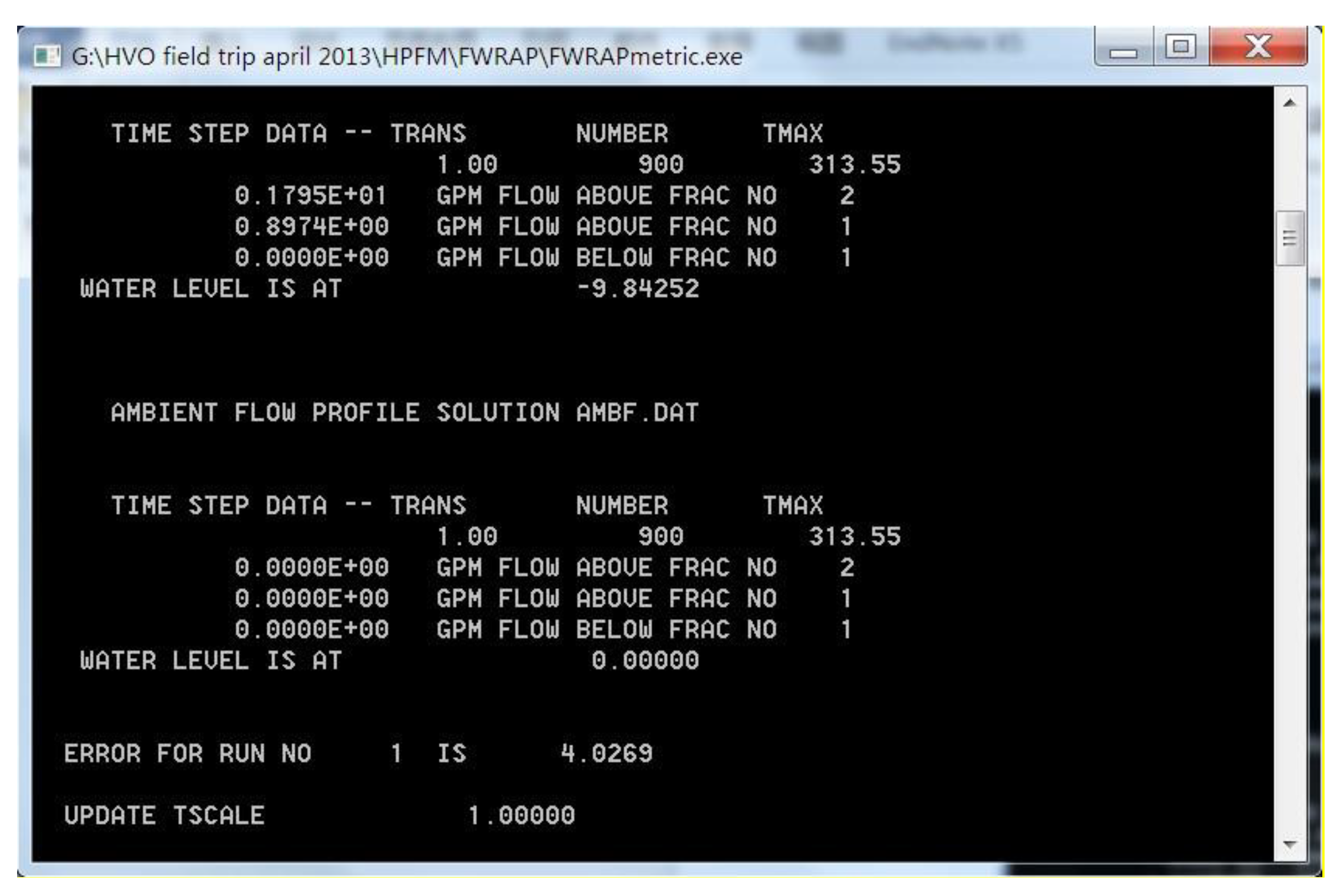
Calculate the total in/outflows under each condition to verify the accuracy of the previous calculation. For example, the total in/outflows of the ambient test should be zero, and the total in/outflows of the injection/pumping test should be equal to the injection/pumping rate.

(2)

Calculate the difference in/outflows between the ambient and injection/pumping conditions; the result should be all negative numbers for the injection condition, and the result should be all positive numbers for the pumping condition.

(3)

Calculate the percentage of initially estimated transmissivity (T₀) of each formation-contained aquifer (i.e., an initial guess of total T₀ of aquifer having flow-producing geological formations), which results from the total in/outflows divided by this fracture’s different in/outflows; the total percentage of T₀ should be 100%.

An example of the subtraction in/outflows analysis based on mass conservation is given in Table 2. While calculating the subtraction of in/outflows, the vital point is that when an injection test is compared to an ambient test, the inflows must be all negative (see all instances in the section of results and discussion); if a pumping test is compared to an ambient test, the outflows must be all positive (see the instance in

Table 3. The in/outflows analysis by mass conservation for borehole A435_R_056.

Zone	Ambient			Injection			Difference between the Ambient and Injection Tests [l/min]	Percentage of T0 * (%)
Depth [m]	Above [l/min]	Below [l/min]	Flow [l/min]	Above [l/min]	Below [l/min]	Flow [l/min]
34	0.00	−1.25	1.25	2.92	1.44	1.48	0.23	8
73	−1.25	0.00	−1.25	1.44	0.00	1.44	2.69	92
Total			0.00			2.92	2.92	100

* T₀ indicates an initially estimated total transmissivity of a fracture-contained aquifer.

). Otherwise, there must be errors in the data, and the percentage of T₀ cannot be calculated, indicating that additional calculation and analysis cannot be carried out further. This data-analysing method of the subtraction in/outflow has been well-developed by Molz et al. [52] and later reapplied by Molz et al. [41].

2.3.3. Groundwater Inversion Modelling

Since the flow rate profile is successfully analysed, groundwater inversion modelling can be implemented to estimate T and far-field H of aquifers having geological formations (e.g., fractures and faults). This task can be achieved using the HPFM appending software in the name of FWRAP provided by Paillet [53], who developed this groundwater inversion analysis for borehole flow rate logging. FWRAP is a computer program that back-calculates each fracture’s T and H under steady-state conditions by the trial-and-error method. It can also be applied to back-calculate specific yield (S_y), specific storage (S_s) and storativity (S) (S = S_y + S_sB, where B is the thickness of a confined aquifer) [7,11,12], in addition to T and H, under an evolution from transient towards steady-state flow conditions.

This theoretical framework and mathematical modelling setup are based on the solution of the slug test developed by Cooper Jr et al. [54] as follows. First, the formulation of borehole flow rate is given by Davis and De Wiest [55]:

$$q_i^a=2\pi T_i(H_i-h^a)\ln \left(\frac{R}{r}\right)$$

(1)

where q_i^a is the measured flow into the borehole from flow-producing zone i under the testing condition a; T_i is the transmissivity of zone i; H_i is the far-field head in the aquifer, h^a is the hydraulic head in the borehole under the testing condition a; R is the distance to the “recharge boundary” or “outer edge” of the flow-producing zone i, and r is the borehole radius. In Equation (1), ln(R/r) can be treated as a constant value, and π is also a constant value; the measured flow q_i^a is proportional to the product of T_i and (H_i − h^a) rather than T_i alone.

Thus, it is clear that only measuring the water flow under one testing condition is insufficient to analyse the flow profile and mass conservation for an identified geological formation. The flow needs to be measured under two quasi-steady conditions: the ambient and the steady-state injection/pumping conditions [47]. Then, Equation (1) can be transformed:

$$q_i^b-q_i^a=2\pi T_i(h^b-h^a)\ln \left(\frac{R}{r}\right)$$

(2)

where q_i^b is the measured flow into the borehole from flow-producing zone i under the testing condition b, and h^b is the hydraulic head in the borehole under the testing condition b. In Equation (2), the value of H_i has been subtracted from Equation (1), and the values of h^a and h^b can be easily measured by the water level detector under both testing conditions of a and b, so the only unknown value is T_i. Then, the quantitative estimation of T_i can be obtained.

In a steady borehole flow system, the water level should have no variation, so the sum of all in/outflow to the borehole should be zero. Using the form of Equation (1), this can be described below.

$${\displaystyle \sum q_i^a}={\displaystyle \sum 2\pi T_i(H_i-h^a)\ln \left(\frac{R}{r}\right)}=0$$

(3)

After rearranging, Equation (3) will be transformed into the following form.

$${\displaystyle \sum T_i{H}_i}=h^a{\displaystyle \sum T_i} \mathrm{or} h^a=\frac{{\displaystyle \sum T_i{H}_i}}{{\displaystyle \sum T_i}}$$

(4)

As T_i and h^a are all known values, H_i can be calculated by the trial-and-error method. The content mentioned above illustrates the calculating procedure of the borehole flow data. Also, it explains why the borehole flow under two different quasi-steady conditions is required in the groundwater inversion modelling theoretical framework.

As FWRAP back-calculates each flow-producing zone’s T and H by the trial-and-error method, this software requires a series of input of parameters and variables: the number of fractures (N) in the borehole (see an instance of fracture characterisation in Table 2), the diameter (D) of the borehole (i.e., the borehole radius r = D/2 in Equations (1)–(3)), the ambient flow (q_i^a) and injection/pumping flow (q_i^b) above each fracture (see Equation (2) and instances in Table 3), the total borehole depth (Z_t), the borehole water level (h_a) under the ambient condition (see Equations (1)–(3)), the water head variation (h_b-h_a) in the borehole between the ambient and the injection/pumping tests (see Equation (2)), the initial guess of the hydraulic head (H_i,0) for each flow-producing zone (see Equations (1), (3) and (4)), the initial guess of the total transmissivity (T₀) of a fracture-contained aquifer (see instances in Table 3), and the initial guess of T_i,0 for each flow-producing zone i (i.e., each percentage of total T₀ for each characterised fracture i, see instances in Table 3).

It should be noted that the in-situ transmissivity (T_i) is obtained by

$$T_i=k_i{H}_i$$

(5)

where k_i is the in-situ hydraulic conductivity for a flow-producing zone i. The corresponding intrinsic permeability (K_i) can be given by

$$K_i=\frac{\mu k_i}{\rho g}$$

(6)

where μ, ρ and g are the borehole fluid dynamic viscosity, density and gravitational acceleration, respectively. In addition, such k_i and K_i for each flow-producing zone are higher than the k_i and K_i of intact soil, rock and coal specimens tested in the laboratory in several orders due to higher q_i through the flow-producing zone i in an aquifer.

The operating interface of FWRAP is shown in Figure 4. First, it can forward model q_i and far-field H_i for each flow-producing zone with the initially guessed values mentioned above. Then, by updating the values of T₀ and T_i,0 through a series of iterations using the trial-and-error method, the inversion analysis succeeds when both modelled values perfectly fit into the measured values, statistically indicated by a minor square difference between the modelled and measured values. The iteration should be continuously carried out until the error is sufficiently small to be accepted by the HPFM-FWRAP practitioners. And after running the FWRAP software, the inverse modelling result can be outputted for further analysis.

2.4. Field-Case Study

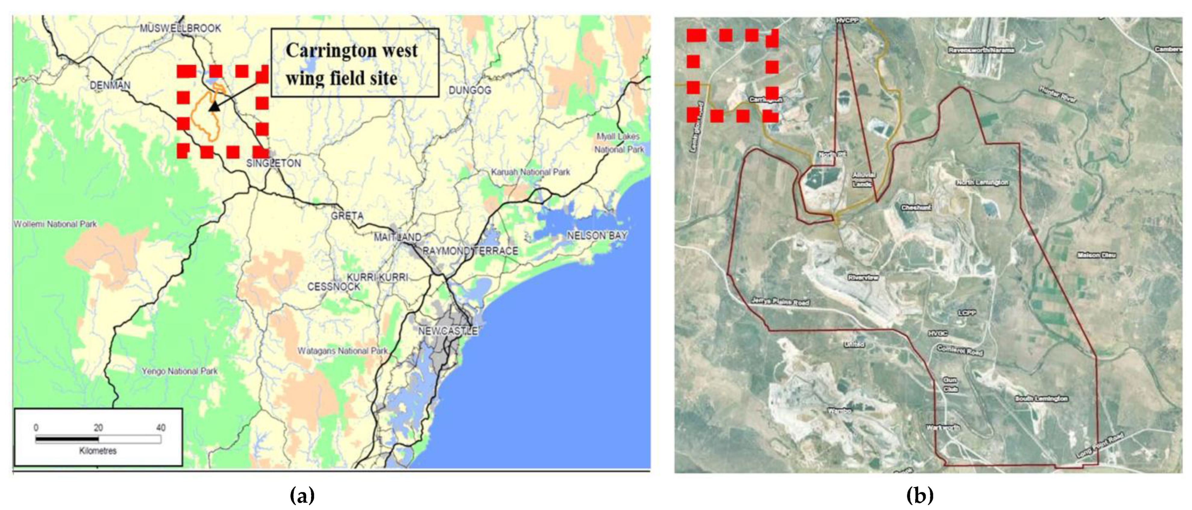
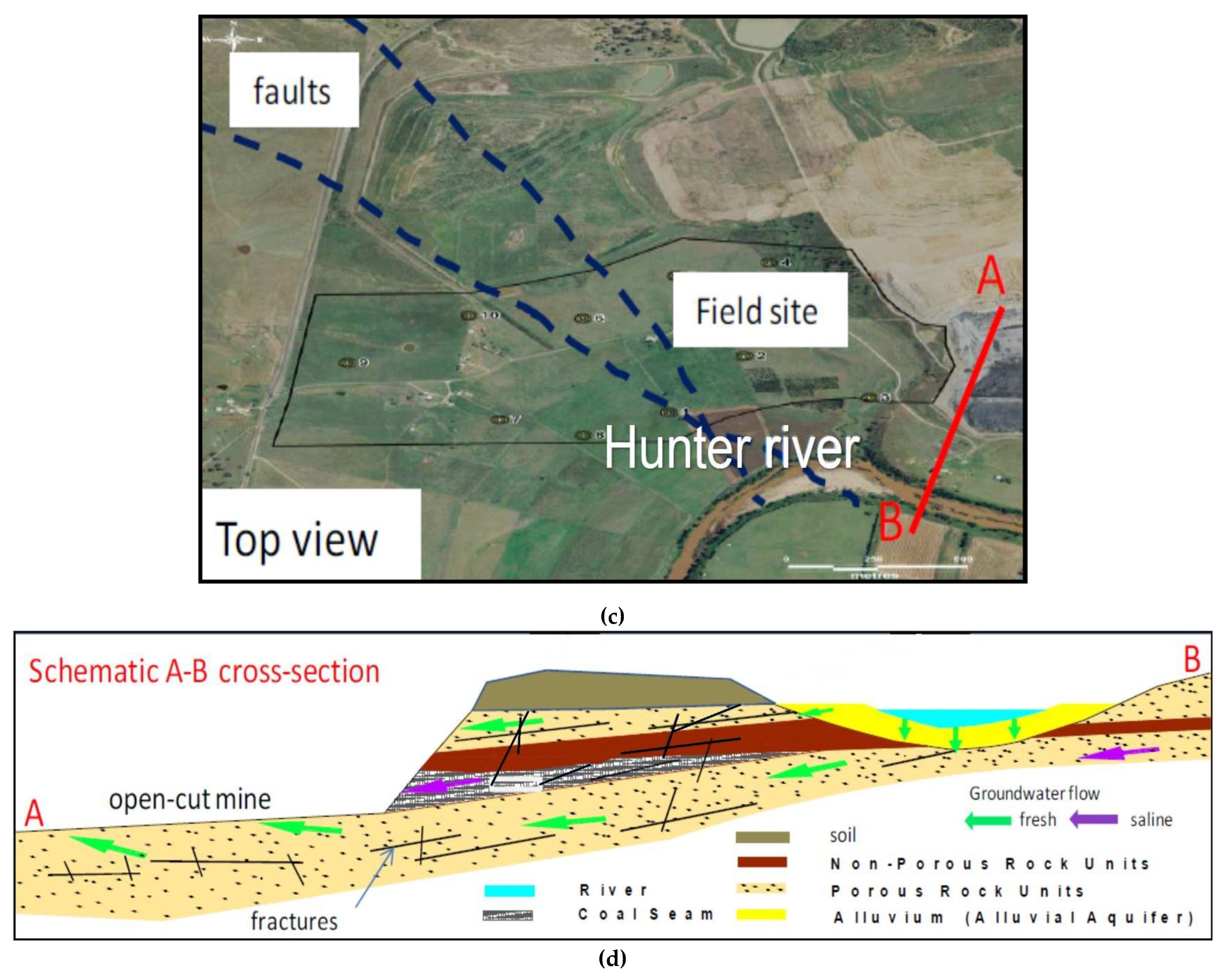
2.4.1. Site Brief

Hunter Valley Operations (HVO) is one of Australia’s major coal mining regions that is located 24 km northwest of Singleton in the Hunter Valley region of New South Wales (NSW), Australia (see Figure 5a,b), and Rio Tinto Coal Australia owns this mining area. It has been operated by Coal & Allied Operations Pty Ltd. [56]. The mining extension zone was located on the north side of the Hunter River, NSW, Australia, as shown in Figure 5c.

Hunter Valley mining adopts the open-cut method instead of underground mining, which will remove the overburdened earth strata above the coal seam (see Figure 5b–d). However, this mining method will require a mass of mining pit drainage and affect the nearby region’s water system, i.e., the adjacent aquifer system and Hunter River (see Figure 5c,d). As more details of the transect A–B are shown in Figure 5d, the effect will appear in two respects: the first is the groundwater level drawdown and water loss in the Hunter River, and the second respect is that the drained water will pass through the coal seam or mix with the water originating from the coal seam. This amount of groundwater will be drained with saline groundwater and finally discharged into Hunter River and nearby creeks. Those discharges will result in severe pollution of the river ecosystem, including the riparian and hyporheic zone [2]. This project will help solve the problem by using the HPFM to measure the in-situ flow rates in the HVO mining extension area’s boreholes and then calculate the T and far-field H of each flow-producing zone in the adjacent aquifer system. These data can further be used in large-scale groundwater modelling.

2.4.2. Challenges in In-Situ Setup of HPFM

As schematically sketched in Figure 5d, the rock beds and coal seams in the selected field site are mainly overburdened with the unconsolidated alluvial soil layers, including paleochannel sediments of gravel, silt and clay, in thickness alternating in the range of 10–25 m, below which there are the shale and sandstone strata to form the unconfined aquifer above the low permeable aquitard. In addition, two fault zones in the northeast and south trends have been previously detected in the west of the selected field site (see Figure 5c). The previously detected faults, potentially expanding faults, and jointing zone adjacent to those faults have been branched from the fault zones. Those geological formations produce the preferential seepage flow conduits between the alluvial sediments and coal seam beds, comprehensively reported by Age Australasian Groundwater & Environmental Consultants Pty Ltd. Bowen Hills, Brisbane, QLD, Australia. [57].

As illustrated in Figure 6a,b, the boreholes drilled to depths of 50–75 m were fitted with an outer steel pipe for borehole-casing in the aforementioned alluvial soil layers (15–24 m beneath the ground surface in Figure 5d). Underneath those soil strata, an inner PVC pipe connected to the upper steel casing was slotted in each borehole. In Figure 6a,b, the diameter of the solid casing in steel is 9.9 cm, and the diameter of the slotted pipe in PVC is 6.5 cm. The void space between the borehole’s inner wall and the casing pipe was backfilled with medium-sized gravel (3–8 mm). This casing strategy was applied to prevent borehole collapse. Most of the selected boreholes had been cased with this approach before the HPFM measurement, except for a few boreholes.

Unfortunately, due to having implemented the borehole casing approach, the slotted pipe diameter was too small to fit the HPFM flow diverter into the selected boreholes. As a result, without using this diverter (see Figure 6a), a certain amount of water was prone to flow outside the detecting probe tip (see Figure 6b). Therefore, prior to any formal flow rate logging by HPFM, the calibration between the detected flow rate and actual in-situ flow rate had to be completed, even though the HPFM in type HFP-2293 had been calibrated by the manufacturer, Mount Sopris Instruments Co., Denver, Colorado, [51], in the laboratory and the field nearby.

2.4.3. In-Situ Calibration

HFP-2293 without a flow diverter was calibrated under the field conditions in the following procedure. First, a regulated volume of water (stored in the white tanks in Figure 2a,b) was injected into each borehole. Then, the flow rates, simultaneously measured by the manual flowmeter and HFP-2293, were compared to derive a calibrating ratio between those, so-defined as the bypass factor of HPFM by Paillet [50].

The borehole profile was compartmented into the solid casing part by steel pipe (see Figure 6a) and the slotted part by PVC casing (see Figure 6b), so the calibration tests could be done in both the solid casing and slotted parts. Figure 6a shows the condition of the calibration test in the solid casing part. When there was no flow diverter around the HPFM probe tip, some water flow would bypass the probe tip downwardly. Hence, there would be a ratio between the actual and measured flow rates. For example, if the injection rate is 4 l/min, and the measured flow is 1 l/min, we could calculate the bypass factor as 4/1 = 4. In addition, because the casing pipe is a solid casing and no water could flow in/out at this part, we did not need to consider the fracture or permeable layer problems while doing the calibration test.

For the calibration test in the slotted part, the situation could be different from the calibration test in the solid casing part. As illustrated in Figure 6b, borehole water could flow out of the casing pipe and stream in the backfilled area. In fact, most water could flow into the backfilled area. Thus, compared to the solid casing part in Figure 6a, less water flow can be measured in the slotted part, and the bypass ratio might be significantly large. For instance, if the injection water flow rate is 4 l/min and the measured water flow rate is 0.2 l/min, the bypass ratio should be 4/0.2 = 20. One crucial point that needs to be noted here is that the flow testing point must be above the first fracture in the slotted area. Otherwise, the water flow will be enormously changed nearby the fracture, and the bypass ratio calculated this way will provide an incorrect value. In order to prevent the calibration from this case, other geological investigation (GI) methods should be utilised to roughly identify the first geological formation before carrying out the flow logging by HFP-2293 without the flow diverter.

Finally, after the bypass ratios were correctly determined for each borehole, those ratios could be individually applied to the flow logging of each borehole in order to correct the HPFM-detected flow rates. Note that the calibration tests were only carried out for the boreholes with casing pipe diameters smaller than the flow diverter, whereas it was not compulsory for other exceptions having no borehole casing.

3. Results and Discussion

3.1. In-Situ Borehole Selection

The first field trip using HPFM in the type of HFP-2293 in this project was held in October 2012. On this field trip, seven boreholes were measured in borehole numbers: A435_C_003, A435_R_043, A435_R_045, A435_R_049, A435_R_051, A435_R_054 and A435_R_060. All of these boreholes were measured by the single-borehole flow measurement method. Figure 7a shows the locations of these boreholes.

The project’s second field trip using HPFM (HFP-2293) was held in April 2013. This field trip measured nine boreholes in borehole numbers: A435_R_040, A435_R_042, A435_R_044, A435_R_045, A435_R_046, A435_R_050, A435_R_051, A435_R_056 and A435_R_059. As listed in

Table 4. The selection of borehole locations in field trips.

Borehole No.	Location
	Latitude	Longitude
A435_C_003 (Figure 14a)	32°29′36.54″ S	150°57′38.45″ E
A435_R_040 (Figure 14e)	32°29′27.89″ S	150°57′31.71″ E
A435_R_042 (Figure 16a)	32°29′28.78″ S	150°57′06.45″ E
A435_R_043 (Figure 14b)	32°29′30.15″ S	150°57′40.93″ E
A435_R_044 (Figure 16b)	32°29′31.24″ S	150°57′15.66″ E
A435_R_045 (Figures 8 and 13)	32°29′32.41″ S	150°57′50.15″ E
A435_R_046 (Figure 14f)	32°29′33.43″ S	150°57′24.84″ E
A435_R_049 (Figure 14c)	32°29′35.69″ S	150°57′34.03″ E
A435_R_050 (Figure 14g)	32°29′36.83″ S	150°57′08.22″ E
A435_R_051 (Figure 16c,d)	32°29′38.05″ S	150°57′43.21″ E
A435_R_054 (Figure 14d)	32°29′41.36″ S	150°57′27.08″ E
A435_R_056 (Figure 3 and Figure 9)	32°29′42.31″ S	150°57′01.85″ E
A435_R_059 (Figure 11)	32°29′44.89″ S	150°57′18.84″ E
A435_R_060 (Figure 15)	32°29′47.03″ S	150°57′46.57″ E

S and E indicate the directions: South and East, respectively.

, all boreholes were measured by the single-borehole flow measurement method. Figure 7b shows the locations of these boreholes.

Moreover, all borehole locations selected in those two field trips (October 2012 and April 2013) are listed in Table 4. For readers’ interests, the borehole locations can be checked using Google Maps or other satellite imaging software with a global navigation system, e.g., the global positioning system (GPS), BeiDou navigation satellite system (BDS), etc.

3.2. In-Situ Calibration for Bypass Ratio

Due to a lack of user experience and unawareness of the complicated situation of borehole casing conditions (see Figure 6a,b) in the first trip, the in-situ calibration tests were not carried out, whereas it was rigorously conducted in the second field trip for the boreholes in numbers: A435_R_040, A435_R_042, A435_R_044, A435_R_045, A435_R_046 and A435_R_050. Following the in-situ calibration procedure introduced in the previous methodology section, the calibrations between the actual flow rate measured by the manual flow meter and the HPFM-measured flow rate during injection tests are given in

Table 5. The selection of borehole locations in two field trips.

Boreholes No.	Depth (m)	Casing Part (Solid or Slotted)	Actual Flow Rate (l/min)	Measured Flow Rate (l/min)	Bypass Ratio (Actual/Detected)
A435_R_040	15	Solid	7.00	1.80	3.90
A435_R_042	20	Slotted	3.00	0.76	3.95
A435_R_042	20	Slotted	3.50	0.96	3.65
A435_R_042	20	Slotted	4.00	1.09	3.67
A435_R_044	18	Solid	3.00	0.89	3.37
A435_R_044	18	Solid	4.00	1.26	3.17
A435_R_044	18	Solid	5.00	1.43	3.50
A435_R_044	20	Slotted	3.00	0.14 *	21.43 *
A435_R_044	20	Slotted	4.00	0.24 *	16.67 *
A435_R_044	20	Slotted	5.00	0.32 *	15.63 *
A435_R_045	15	Solid	16.89	3.67	4.60
A435_R_046	17	Solid	3.00	0.91	3.30
A435_R_046	17	Solid	4.00	1.16	3.45
A435_R_046	17	Solid	5.00	1.44	3.47
A435_R_046	19	Slotted	3.00	0.17*	17.65 *
A435_R_046	19	Slotted	4.00	0.16 *	25.00 *
A435_R_046	19	Slotted	5.00	0.16 *	31.25 *
A435_R_050	17.5	Solid	1.50	0.42	3.57
A435_R_050	17.5	Solid	2.00	0.51	3.92
A435_R_050	17.5	Solid	2.50	0.73	3.42
A435_R_050	17.5	Solid	3.00	0.89	3.37
A435_R_050	17.5	Solid	4.00	1.23	3.25
A435_R_050	27	Slotted	1.50	0.05 *	30.00 *
A435_R_050	27	Slotted	2.50	0.03 *	83.33 *
A435_R_050	27	Slotted	4.00	0.23 *	17.39 *
Mean	–	–	–	–	3.60
SD	–	–	–	–	±0.35

* Note that those values are incorrect due to unreasonable flow rates by HPFM, so they are abandoned for mean and SD.

for all selected boreholes.

According to the calibration tests listed in Table 5, it is clear that for the solid casing part, their bypass ratios were in the range of 3–5, while for the slotted part, their bypass ratios were in the range of 3–85. However, it should be noted that by comparing the values of A435_R_046 and A435_R_050 for the slotted part, their bypass ratios were far over the reasonable range of 3–5. Actually, this range has been well accepted with all tests for the solid casing part and even A435_R_042 for the slotted part. Apparently, those unreasonable bypass ratios of A435_R_046 and A435_R_050 for the slotted part were attributable to the unreliable flow rates measured by HPFM. After eliminating all those irrational values, it is possible to determine the in-situ bypass ratio for those borehole tests from 3.17 to 4.60, which agrees with Busse et al. [6]. Therefore, to apply a reasonable bypass ratio for all borehole flow rate measurements by HPFM, the mean value of 3.60 with a standard deviation (SD) of ±0.35 were adopted in the following flow rate calibration. Note that this mean value and SD have not included the aforementioned unreliable bypass ratio.

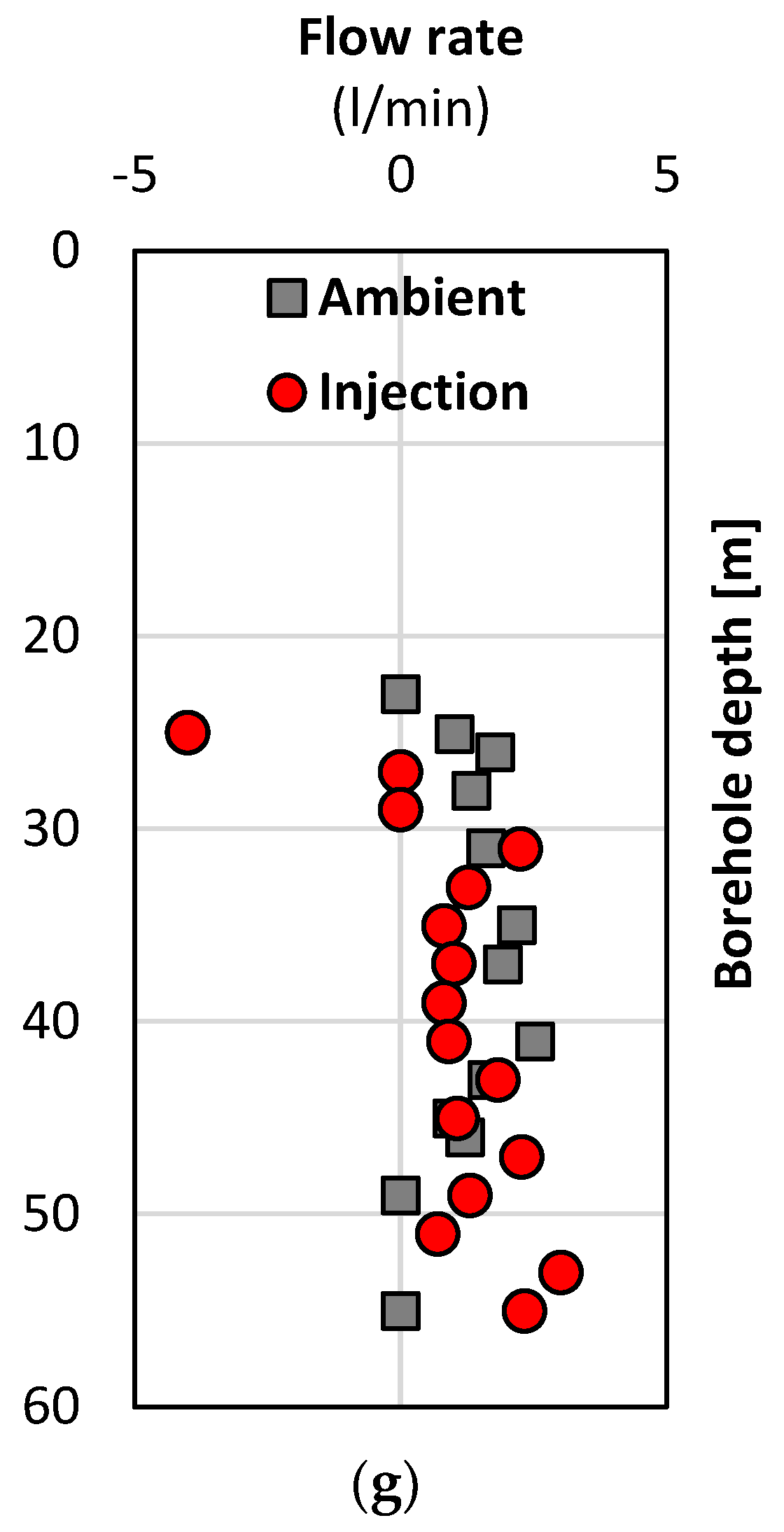
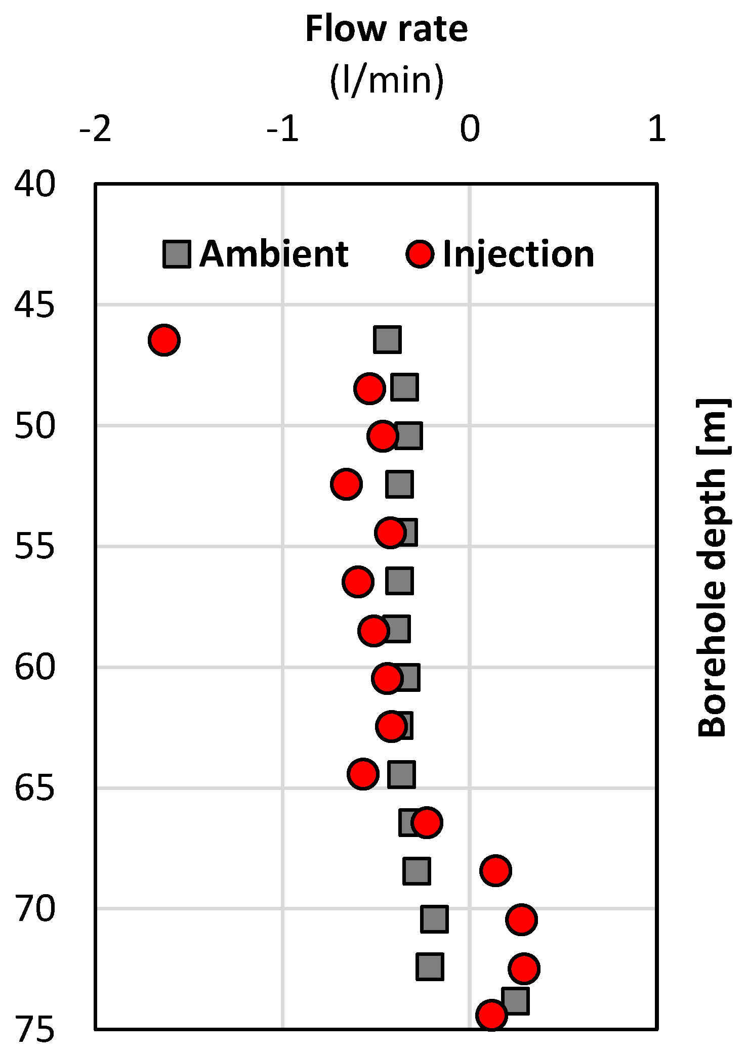
3.3. Positive and Verified Outcomes and Fracture Analysis

During the first and second field trips, there were many positive and verified outcomes from applying HPFM and post-analysis. Therefore, those successes of in-situ HPFM measurements are illustrated in the following content with all essential analysing principles to be strictly complied with.

3.3.1. Borehole A435_R_045 (Trip 2)

The in-situ flow rate logging for borehole A435_R_045 in the second field trip is shown in Figure 8. Based on the reasonability of data scatter introduced in the previous methodology section, all injection test datasets should be on the left-hand side of all ambient test datasets (if the pumping test is carried out, the pumping test data should be on the right-hand side of the ambient test data, although it was not conducted in this work). In Figure 8, despite two anomalies at 21 m and 27 m for the injection test (highlighted by blue boxes) possibly caused by measuring errors, most data points follow the aforementioned principle, so this flow rate profile can proceed with fracture location identification.

The geological formations, such as fractures and faults, can usually be indicated by significant variations in in-situ flow rates. For example, as seen in Figure 8, it is apparent that the fractures could exist in depths of 17 m and 28 m. Then, the average flow rate for each zone delimited by two previously identified fractures could be calculated in order to plot the estimated flow rate profile with an average flow rate assigned to each delimited zone. The estimated flow rate profile fitting through the original data points can be observed in Figure 8. Unfortunately, there was no chance to confirm these fracture location estimations due to unavailable access to other geological investigation (GI) methods for this borehole. Nonetheless, although the estimated fracture location cannot be fully verified, this flow rate profile as a positive outcome from HPFM logging is still analysable.

Table 6. Fracture identification and in/outflow analysis for the borehole: A435_R_045 (Trip 2).

Zone	Ambient			Injection			Difference between an Ambient and an Injection [l/min]	Percentage of T0 * (%)
Depth [m]	Above [l/min]	Below [l/min]	Flow [l/min]	Above [l/min]	Below [l/min]	Flow [l/min]
17	−4.14	0.00	−4.14	−7.65	0.00	−7.65	−3.50	87.71
28	−0.00	−4.14	4.14	−4.00	−7.65	3.65	−0.49	12.29
Total			0.00			−4.00	−4.00	100.00

* T₀ indicates an initially estimated total transmissivity.

delivered the inflow analysis of borehole A435_R_045 after the fracture identification and flow rate profile analysis. With the fracture locations previously estimated, the flow rates above and below each fracture could be calculated according to the rules interpreted in the methodology section. In addition, as injection tests were conducted to this borehole in our field trip instead of pumping tests, the inflow between ambient and injection tests should be negative values instead of positives. In Table 6, the difference between ambient and injection tests provided all negative values without any positive values, so the percentage of initially estimated transmissivity (T₀) with other settings (fracture locations, averaged flow rates, etc.) could be successfully determined as the initial guess of coefficients and input variables for the following groundwater inversion modelling.

Eventually, groundwater inversion modelling was carried out using FWRAP with all inputting coefficients and initial guesses, as listed in the subsection of groundwater inversion modelling. It should be noted that most parameters and coefficients can be provided from the borehole dimension and the post-analysis of HPFM flow rate logging. Still, the initial guesses in terms of fracture far-field head (H₀ -> H) and fracture transmissivity (T₀ -> T) have to be updated by the trial-and-error method until the minor square difference between the modelled and measured values can be accepted by experienced practitioners (as minimum as possible). So far, no optimisation algorithm has been developed to replace the trial-and-error method with comprehensive statistical analysis. The hydraulic characterisation for borehole A435_R_045 was finally provided in

Table 7. Back-calculating T and far-field H for the borehole (A435_R_045 (Trip 2)) by FWRAP.

Detected Flow-Producing Zone in Depth (m)	Transmissivity (m2/day)	Water Level below Ground Surface in Depth (m)
17	1.61	10.14
28	0.27	39.71

, where the T of the fracture in the depth of 17 m was higher than that in the depth of 28 m (1.61 m²/day > 0.27 m²/day), and the corresponding fracture H in 17 m was 29.57 m more elevated than that in 28 m (10.14 m < 39.71 m in depth from ground surface).

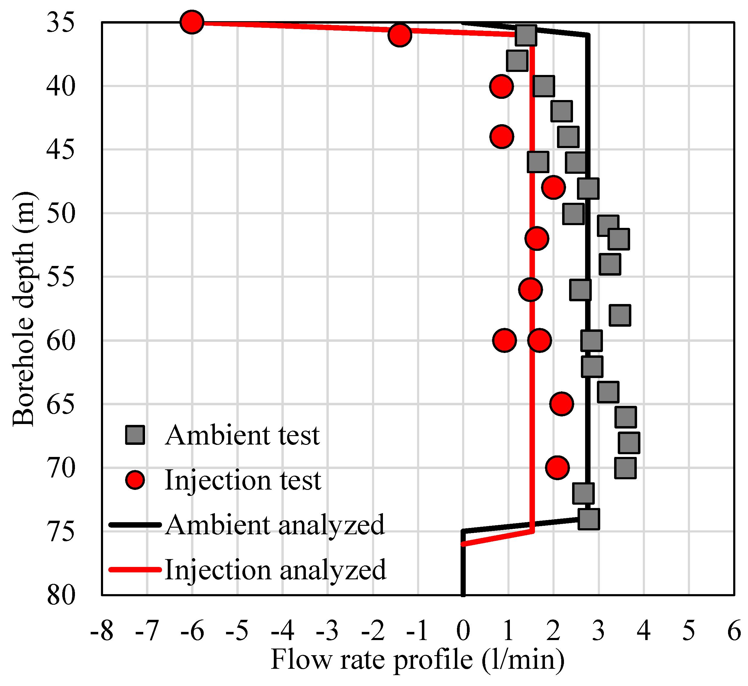
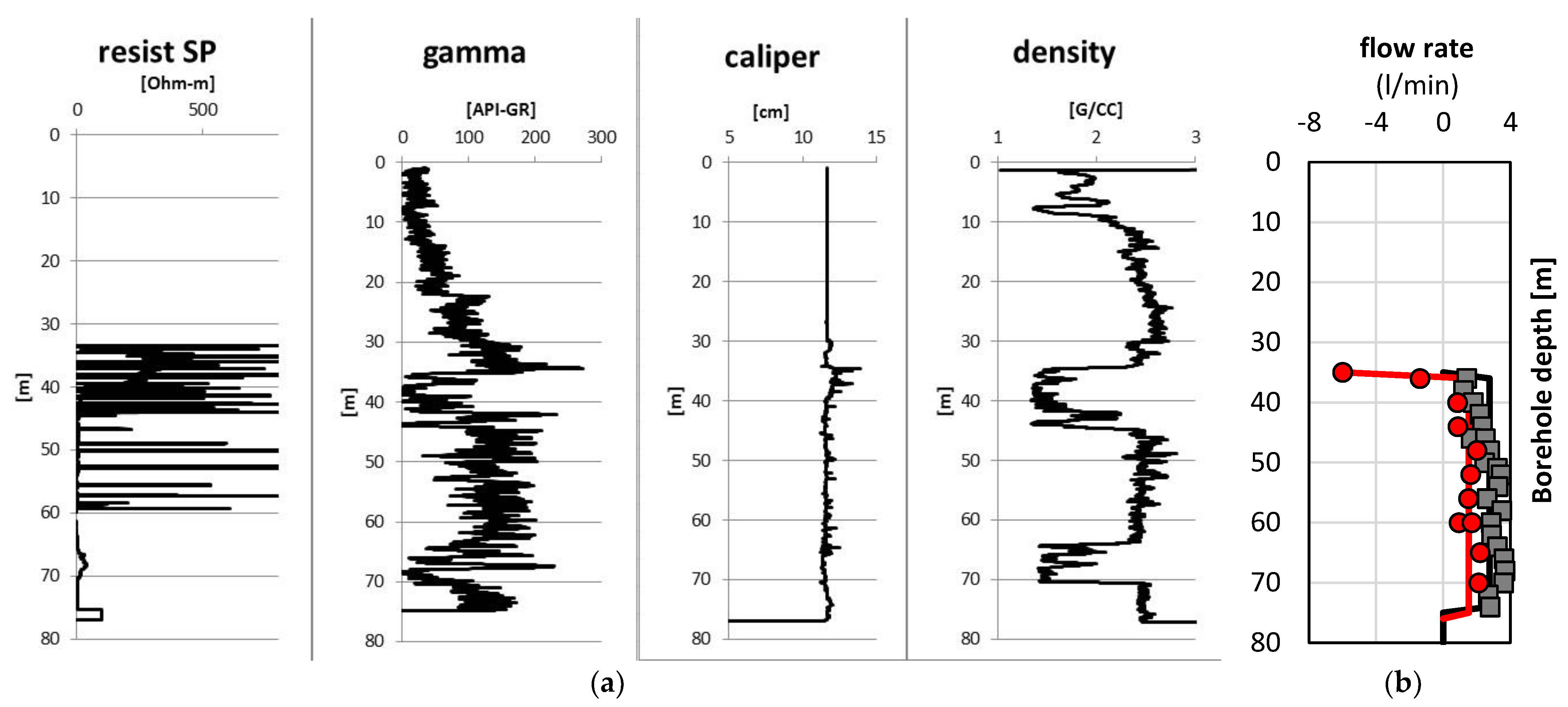
3.3.2. Borehole A435_R_056 (Trip 2)

The in-situ flow rate logging for borehole A435_R_056 in the second field trip is shown in Figure 9. Based on the reasonability of data scatter introduced in the previous methodology section, all injection test datasets should be on the left-hand side of all ambient test datasets, whereas the pumping test data should be on the right-hand side of the ambient test data. In Figure 9, there was no observation of any measuring errors because all injection test data points were on the left-hand side of ambient test data points. As a result, all data points follow the reasonability of the data scatter mentioned above, and this flow rate profile can therefore proceed with fracture location identification.

The flow rate changes indicate the possible existence of flow-producing geological formations. Because of this, significant variations in in-situ flow rates in the borehole A435_R_056 could be observed for the depth of 36 m and 75 m in Figure 9. Then, the average flow rate for each zone delimited by two estimated fracture locations could be calculated in order to plot the estimated flow rate profile by assigning an average flow rate to each delimited zone. As a result, the estimated flow rate profile fitted into the original data points can be shown in Figure 9 and Figure 10b. Moreover, due to available access to other GI methods (see Figure 10a), including in-situ electrical resistance (resist SP), gamma ray (gamma), calliper and density logging, these fracture locations were successfully identified by the HPFM post-analysis. More explicitly, the facture locations could be observed at 36 m and 75 m in Figure 10a, b, where not only the flow rate significantly varied, but other GI loggings (e.g., density, resistivity, gamma, calliper) also did. Other GI methods have successfully verified the fracture location identification by HPFM logging.

Table 8. Fracture identification and in/outflow analysis for the borehole: A435_R_056.

Zone	Ambient			Injection			Difference between an Ambient and an Injection [l/min]	Percentage of T0 * (%)
Depth [m]	Above [l/min]	Below [l/min]	Flow [l/min]	Above [l/min]	Below [l/min]	Flow [l/min]
36	0.00	2.76	−2.76	−6.20	1.53	−7.73	−4.96	80.04
75	2.76	0.00 **	2.76	1.53	0.00	1.53	−1.24	19.96
Total			0.00			−6.20	−6.20	100.00

* T₀ indicates an initially estimated total transmissivity; ** 0.00 indicates reaching borehole bottom.

presents the inflow analysis of borehole A435_R_056 after the successful fracture location identification and flow rate profile analysis. With the fracture locations fully confirmed by HPFM flow analysis and other GI methods, the flow rates above and below each fracture were additionally analysed based on the analysing principles in the methodology section. In this field trip, the injection tests were carried out to this borehole rather than pumping tests, so the inflow between ambient and injection tests should be negative instead of positive. In Table 8, the difference between ambient and injection tests exhibited all negative values without positive ones. Therefore, the percentage of T₀ combined with other previously determined settings (fracture locations, averaged flow rates, etc.) could be successfully estimated as input coefficients and variables for the back-calculation of T and far-field H of all detectable fractures by FWRAP.

Last, groundwater inversion modelling was implemented via FWRAP with all inputting coefficients and initial guesses, as listed in the subsection of groundwater inversion modelling. Through continuously updating the far-field H by the trial-and-error method (H₀ -> H), the minor square difference between the modelled and measured values could finally be accepted (usually the minimum value compared to other outcomes). The hydraulic characterisation for borehole A435_R_056 was eventually presented in

Table 9. Back-calculating T and far-field H for the borehole (A435_R_056) by FWRAP.

Detected Flow-Producing Zone in Depth (m)	Transmissivity (m2/day)	Water Level below Ground Surface in Depth (m)
36	7.78	36.09
75	0.07	30.79

. In Table 9, the T of the fracture of 36 m was much greater than that of 75 m (7.78 m²/day > 0.07 m²/day), and the finally determined far-field H for the fracture in the depth of 36 m was 5.20 m lower than that in the depth of 75 m (36.09 m < 30.79 m in depth from ground surface).

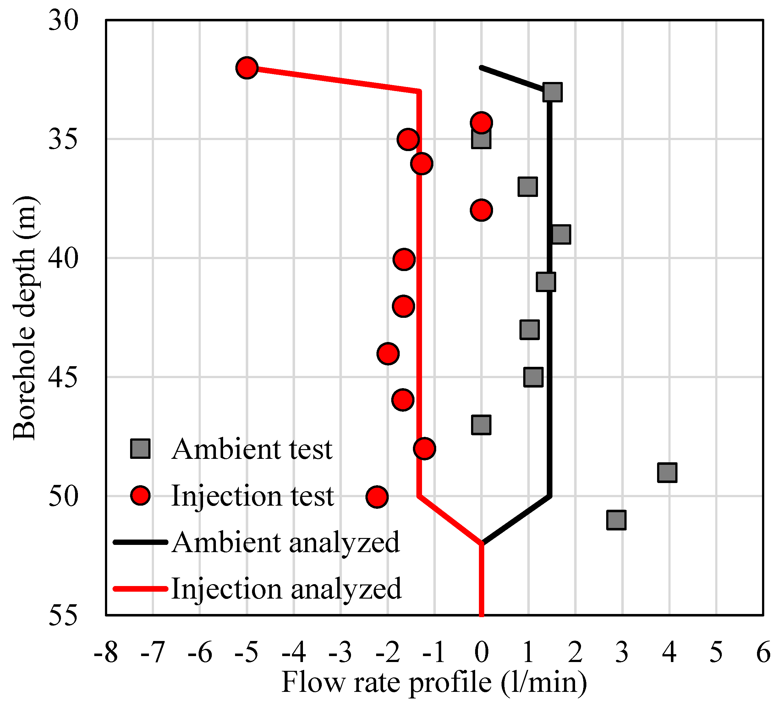
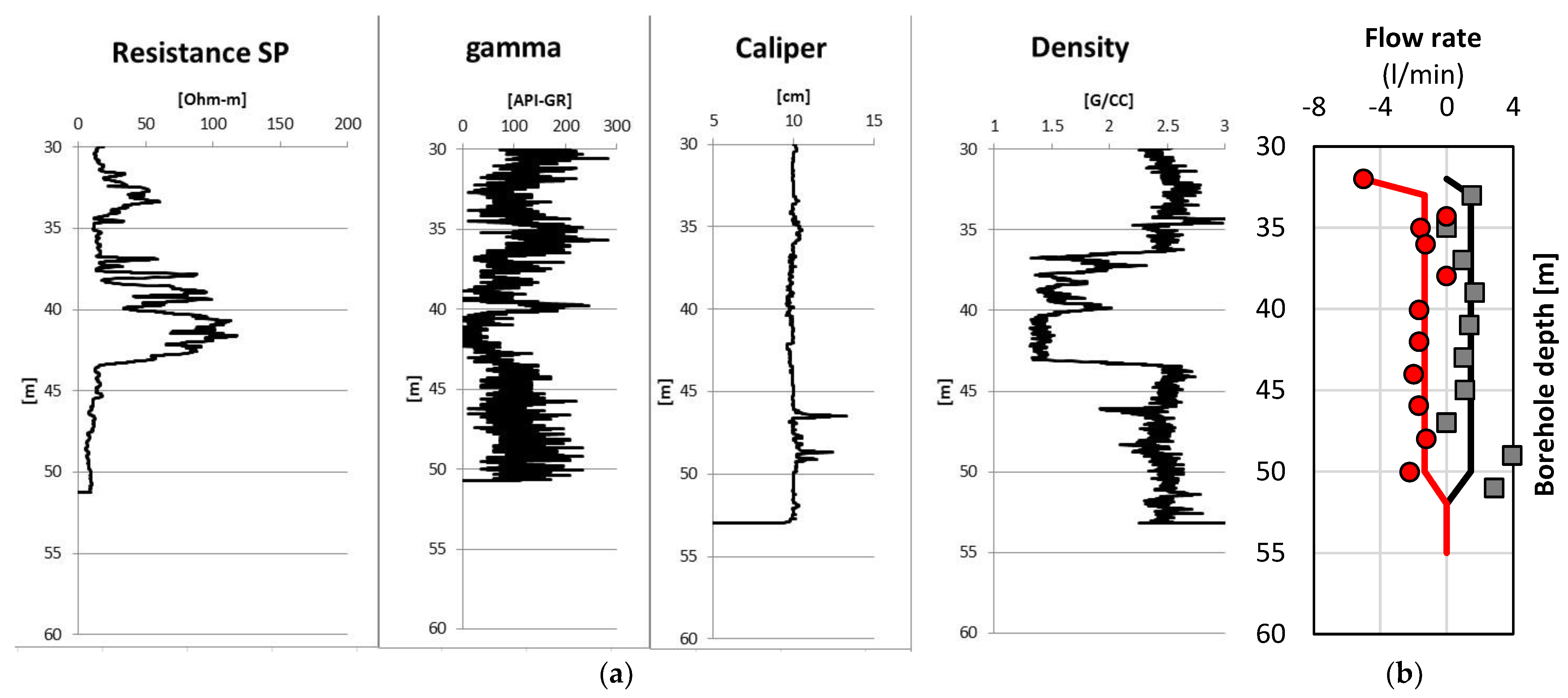
3.3.3. Borehole A435_R_059 (Trip 2)

The in-situ flow rate logging for borehole A435_R_059 in the second field trip is shown in Figure 11. Based on the rationality of data scatter repeatedly mentioned above, all injection and pumping test datasets should be on the left-hand and right-hand sides of all ambient test datasets, respectively. Here, Figure 11 does not show any irrational errors, as all data points of injection tests were on the left-hand side of ambient tests. Since all data points complied with the reasonability of the data scatter, this flow rate profile could be further processed for fracture location identification.

Due to significant changes in flow rates at 33 m and 52 m, there might be two fractures for the borehole A435_R_059 (see two abnormities at 33 m and 52 m in Figure 11). Then, the estimated flow rate profile in the form of average flow rates assigned to the zones delimited by already-known fractures could be plotted to provide a pair of flow rates above and below each identified fracture, respectively, for the latter in/outflow analysis. As a result, the estimated flow rate profile fitted through the data scatter was depicted in Figure 11 and Figure 12b. Furthermore, with access to standard GI methods, these fracture locations estimated by the HPFM post-analysis were reconfirmed by those standard GI methods (see Figure 12a). More explicitly, the facture locations could be observed at 33 m and 52 m in Figure 12a,b, where not only the flow rate significantly varied, but other GI loggings (e.g., density, resistivity, gamma, calliper) also did. Other GI methods have successfully verified the fracture location identification by HPFM logging. However, the fracture locations at 37 m and 44 m (see Figure 12a) could not be identified from the flow rate logging by HPFM. Possible reasons for such fewer variations of flow rates around those fractures could be their much lower hydraulic conductivities compared to the other two identified by HPFM logging and post-analysis. This also demonstrates that HPFM logging can only assist in determining the water-producing zone formed by hydraulic conductive geological formations. Still, not all fracture and fault zones are conductive and detectable.

After successfully identifying fracture locations followed by the flow rate profile analysis, the inflow analysis of borehole A435_R_059 was obtained in

Table 10. Fracture identification and in/outflow analysis for the borehole: A435_R_059.

Zone	Ambient			Injection			Difference between an Ambient and an Injection [l/min]	Percentage of T0 * (%)
Depth [m]	Above [l/min]	Below [l/min]	Flow [l/min]	Above [l/min]	Below [l/min]	Flow [l/min]
33	0.00	1.45	−1.45	−5.00	−1.33	−3.67	−2.23	44.52
52	1.45	0.00 **	1.45	−1.33	0.00	−1.33	−2.77	55.48
Total			0.00			−5.00	−5.00	100.00

* T₀ indicates an initially estimated total transmissivity; ** 0.00 indicates reaching borehole bottom.

. With known fracture locations, the flow rates above and below each fracture were further analysed based on the principle of mass conservation. In addition, in the field trip in April 2013, the ambient and injection tests were carried out to this borehole, so the difference between the two tests should be negative, which could be confirmed by the values in Table 10. Henceforth, the estimation of the percentage of T₀ succeeded.

Finally, the inversion analysis of T and far-field H of all fractures was completed using FWRAP with all inputting coefficients and initial guesses. After iteratively updating the far-field H by the trial-and-error method (H₀ -> H), the differences between the simulated and detected values could eventually achieve the minimum value compared to other iterations. The seepage property determination for borehole A435_R_059 was summarised in

Table 11. Back-calculating T and far-field H for the borehole (A435_R_059) by FWRAP.

Detected Flow-Producing Zone in Depth (m)	Transmissivity (m2/day)	Water Level below Ground Surface in Depth (m)
33	1.05	34.17
52	1.28	30.07

. Table 11 shows that the T of the fracture at 33 m was a little lower than that at 52 m (1.05 m²/day > 1.28 m²/day), and the final estimation of fracture H at 33 m was 4.1 m lower than that at 75 m (34.17 m < 30.07 m deep from ground surface).

3.4. Negative Outcomes and Reflection

During the first and second field trips, there were many adverse outcomes from applying HPFM and post-analysis. Those unsuccesses of in-situ HPFM measurements are summarised in the following content, reflecting possible mistakes and user experience.

3.4.1. Comparison between Unanalysable and Analysable Datasets

To demonstrate the difference between successful and unsuccessful HPFM measurements, the in-situ flow rate profiles of borehole A435_R_045 were measured separately by HPFM in the field trips of October 2012 and April 2013, as plotted in Figure 13a,b. According to the reasonability of data scatter introduced in the previous methodology section, all injection test datasets should be on the left-hand side of all ambient test datasets (if a pumping test is carried out, the pumping test data should be on the right-hand side of the ambient test data). Based on this principle, it is evident that the flow rate profile in Figure 13a is unreasonable because it violates the rationality of datasets for comparing ambient and injection tests.

Moreover, those datasets provided flow rates within a range of −0.5–0.5 l/min, much smaller than the measuring range of HPFM in product code HFP-2293 (the minimum of the HPFM measuring range at 0.113 l/min and corresponding measuring accuracy of 15% (extremes) equivalent to 0.5508 l/min in Table 1). Even though Busse et al. [6] reported that the minimum measuring scale could achieve 0.5 l/m [44], this measuring range of borehole A435_R_045 was even smaller than ±0.5 l/min. Hence, this HPFM measurement failed, so it could not proceed further.

In contrast, the flow rate profile of the borehole A435_R_045 in the second trip (see Figure 13b) fundamentally follows the principle mentioned above, as the majority of injection test datasets are on the left-hand side of ambient test datasets. Therefore, its HPFM post-analysis regarding fracture location estimation and in/outflow analysis has been successfully implemented in Figure 8 and Table 6, followed by groundwater inversion modelling in Table 7.

The reasons resulting in such failure for the first trip could be attributable to a lack of calibration procedure and a possible hardware fault of HFP-2293 that the manufacturer had resolved through the repairment and off-site and laboratory calibration. Without adding a flow diverter in the centre of the HPFM probe tip, the HPFM-detected flow rate was not actually an in-situ flow rate in the borehole at a depth of fractures but a flow rate of cross-sectional flow through the probe tip inside the fine-mesh (see Figure 1a). Unless the in-situ calibration tests were rigorously carried out, it would be impossible to detect the in-situ flow rate by HPFM.

Besides, Busse et al. [6] also pointed out that if there was no flow diverter on the probe tip due to the borehole diameter being smaller than the diverter diameter, there might be possible turbulence around the thermistors during the water flow through the cross-section of the probe tip. The spurious flow rates (see Figure 13a), including both weak-up and weak-down flow conditions (the upward flow in positive value and the downward flow in negative value), could result from the buoyancy effect on the HPFM probe, which has been reported by Williams and Paillet [58].

Based on the reflection analysed above, it is possible to conclude that it is always better to add the flow diverter to divert the water flow through the probe tip effectively; in addition, even if such a diverter is applied, it is also more rigorous to carefully carried out the in-situ calibration tests in order to determine the in-situ bypass ratio for each borehole, depending on the borehole diameter. When the flow diverter cannot fit into the borehole, such a calibration test must be conducted for bypass ratio determination. Even if this calibration is carried out, there could be a potential failure of flow detection due to insufficient water flow through the cross-section of the HPFM probe tip.

3.4.2. Totally Unanalysable Datasets

Several more failure cases of borehole flow rate logging by HPFM are demonstrated in Figure 14. For instance, the flow rate profiles of the boreholes A435_C_003, A435_R_043, A435_R_049 and A435_R_054 in Figure 14a–d show all measured flow rates (−0.5 l/min < q < 0.5 l/min) within the minimum detectable flow rate of HFP-2293 (0.113–3.785 l/min with measuring accuracy in extremes (15%, 0.5508 l/min) in Table 1). This failure could be due to insufficient water flow through the cross-section of the HPFM probe tip without the flow diverter. Despite those boreholes in Figure 14a–d, other cases in Figure 14e–g provide reasonable ranges of borehole flow rates.

However, there are other irrational issues in those cases, as some or most of their injection test datasets, supposed to be on the left-hand side of ambient test datasets, are on the right-hand side of those (see Figure 14b–g) which are all unreasonable in terms of their correct flow directions. The phenomenon of spurious flow can also be observed in those failure cases (see Figure 14e,g).

Based on the initial assessment above, all flow rate profiles reported in Figure 14 cannot initially be used to identify the fractures with assistance from other GI methods. Also, there will be no chance to carry out further the subsequent in/outflow analysis around identified fractures based on mass conservation and the final groundwater inversion analysis.

3.4.3. Partially Unanalysable or Analysable Datasets

An instance of partially unanalysable or analysable datasets is plotted in Figure 15. It shows the flow rate profile of borehole A435_R_060 in the first field trip (October 2012). Most of these datasets follow the principle that the injection test datasets are on the left-hand side of the ambient test datasets, except for the flow rates at depths below 66 m. It also seems to be able to characterise the borehole locations at 45 m and 66 m by checking the significant variations in the flow rate profile.

Nevertheless, due to an incomplete rational flow rate profile, there is no chance to accurately determine each pair of flow rates above and below each identified fracture, particularly for depths below 66 m where the injection test datasets are on the right-hand side of the ambient test datasets. Consequently, the in/outflow analysis can only be done for the fracture at 45 m based on mass conservation, but it fails at 66 m. Specifically, without a complete set of correctly estimated in/outflow rates around fractures and percentages of T₀, there is a lack of input coefficients in the final groundwater inversion analysis.

Furthermore, such an upward flow in an unexpectedly reversed flow direction, indicated by the injection test datasets on the right-hand side of the ambient test datasets, could be attributed to the borehole casing by steel or PVC pipe with backfilled gravel (the solid casing and slot parts in Figure 6a,b). As illustrated in Figure 6a,b, there might be a certain amount of water streaming down through the backfilled gravel casing part and finally circulating through the borehole bottom to supply an upward flow at the bottom part of the borehole A435_R_060. Such cases have been reported by Busse et al. [6] without any demonstrations of in-situ flow rate profile.

However, this backfilling-induced flow circulating at the borehole bottom is not encountered, leading to the failure of in/outflow analysis every time. Paillet et al. [48] have successfully shown many available flow rate profiles detected under such casing conditions, even though the flow rate through the backfilled gravel cannot be measured using the HPFM technique. Hence, in order to more accurately measure in-situ flow rates in boreholes, it is also recommended to apply HPFM without borehole casing, as Busse et al. [6] did in the mining extension zone of Hail Creek Mine, Queensland, Australia. Nonetheless, note that the non-casing boreholes are more vulnerable to borehole collapsing, inducing other adverse effects on in-situ HPFM measurement [6], such as suspension clogging sensors in the probe tip and fine particles advection in borehole flow, etc.

3.4.4. Fracture-Identifiable Datasets with Apparent in/Outflow Errors

The last group of failure cases of the HPFM borehole measurement in Figure 16 has identifiable fractures in their flow rate profiles (available in

Table 12. Fracture identification and in/outflow analysis for the borehole: A435_R_042, A435_R_044, A435_R_051 (Trip 1) and A435_R_051 (Trip 2).

Zone	Ambient			Injection			Difference between an Ambient and an Injection [l/min]	Percentage of T0 * (%)
Depth [m]	Above [l/min]	Below [l/min]	Flow [l/min]	Above [l/min]	Below [l/min]	Flow [l/min]
Borehole A435_R_042
21	0.00	0.21	−0.21	−4.08	−0.25	−3.83	−3.62	88.79
35	0.21	2.89	−2.68	−0.25	0.30	−0.55	2.13	−52.05
60	2.89	0.00	2.89	0.30	0.00	0.30	−2.58	63.27
Total			0.00			−4.08	−4.08	100.00
Borehole A435_R_044
18	0.00	6.53	−6.53	−4.00	−2.67	−1.33	5.20	−130.02
25	6.53	3.74	2.78	−2.67	−4.05	1.37	−1.41	35.25
51	3.74	3.65	0.10	−4.05	1.82	−5.86	−5.96	148.92
60	3.65	0.00	3.65	1.82	0.00	1.82	−1.83	45.85
Total			0.00			−4.00	−4.00	100.00
Borehole A435_R_051 (Trip 1)
34	1.64	−0.34	−1.98	0.12	−0.58	0.70	2.68	120.00
51	−0.34	−0.68	0.34	−0.58	−1.07	0.49	0.15	7.00
54	−0.68	−0.40	−0.28	−1.07	−0.32	−0.75	−0.47	−21.00
58	−0.40	−0.24	−0.16	−0.32	−0.03	−0.29	−0.13	−6.00
Total			−2.09			−0.26	2.24	100.00
Borehole A435_R_051 (Trip 2)
36	0.00	−0.73	0.73	−0.18	−1.08	0.90	0.17	−94.12
58	−0.73	−0.08	−0.65	−1.08	−0.13	−0.96	−0.30	166.39
67	−0.08	0.00	−0.08	−0.13	0.00	−0.13	−0.05	27.72
Total			0.00			−0.18	−0.18	100.00

* T₀ indicates an initially estimated total transmissivity, and the grey-shading area indicates a violation of mass conservation of water flow for an identified geological formation.

), while the inflow and outflow above and below each identified fracture, respectively, cannot output a reasonable flow difference between ambient and injection tests, as highlighted in Table 12. In another expression, although each flow rate logging by HPFM can help the HPFM practitioner roughly estimate the fracture locations (provided in Table 12), the inflow and outflow around a given fracture totally violate the principle of mass conservation (see the highlights of positive values in Table 12).

Those highlights of positive values in Table 12 indicate the fracture in/outflow tested by injection test is not on the left-hand side of that tested by the ambient test but the right-hand side of that tested by ambient tests. For example, the absolute values of the downward flow (in negative flow rates) by injection test are smaller than that by ambient test (also in negative flow rates) (see Borehole A435_R_042 and Borehole A435_R_044 in Table 12). For other cases, the injection tests produce an upward flow (in positive flow rates), while the ambient tests produce a downward flow or an upward flow smaller than the upward flow by injection tests (see Borehole A435_R_051 (Trip 1 and Trip 2) in Table 12). As a result, the flow differences between ambient and injection tests can exhibit positive values, and summing up such differences can even yield a positive value for the total (see the highlights for Borehole A435_R_051 (Trip 1) in Table 12), consequentially leading to the irrational values of the percentage of T₀ (see all highlights in Table 12).

The reasons causing such failure of in/outflow analysis around fractures could be mainly due to applying HPFM without adding the flow diverter on the probe tip. Without such a diverter, spurious flow could be generated by the aforementioned turbulence, and insufficient cross-sectional flow through the probe tip would occur. In fact, applying HPFM without the diverter could perform relatively well for a few previously mentioned cases with the bypass ratio provided by the in-situ calibration tests. However, it is crucial to note that the in-situ calibration can only obtain an average value of bypass ratio with a standard deviation. More specifically, when this diverter is not used, the more water flow bypasses the probe tip, the higher the bypass ratio on average and the possibly higher the standard deviation to this average. Therefore, the uncertainties resulting from more bypass flow could be potentially magnified without such a flow diverter on the probe. When such uncertainties are hidden and embedded into a few flow rate data points crucial to the analysis of the in/outflow around an identified fracture, the mass conservation violation will be manifested as the highlighted positive values in Table 12. It should be noted that there are two cases of violation of mass conservation for in/outflow analysis: (1) the flow differences in positive values between ambient and injection tests (reported in Table 12), or (2) the flow differences in negative values between ambient and pumping tests, which is not shown in this field-case study.

Therefore, if the in-situ testing situation allows fitting the flow diverter into boreholes without any clogging issues, it is always better to accurately install the diverter on the probe tip than not install it. Also, the in-situ calibration tests should be carried out, even if the diverter is installed, because the diverter only helps to divert the borehole water flowing through the probe tip efficiently. It cannot guarantee zero bypassing flow around the probe tip [6,50].

4. Summary and Reflections

Groundwater flow model at large-scale needs comprehensive geological investigation (GI) to precisely simulate groundwater dynamics during the mining operation. With the presence of faults, fractures, cleats and joints in the overburdened rock strata over coal seam beds, the in-situ borehole flow rate logging can facilitate the estimation of the in-situ far-field hydraulic head and transmissivity (i.e., hydraulic conductivity and intrinsic permeability). In this paper, the heat pulse flowmeter (HPFM) is methodologically introduced and practised for GI in the Hunter Valley Operations (HVO) mining extension zone, New South Wales, Australia. Based on both positive and negative outcomes provided by HPFM measurements, in terms of user experience of the advantages and disadvantages of practising HPFM in the field, as well as constructive recommendations, this field trip study could be summarized in the following points:

(1)

HPFM is a powerful flow measuring technique developed for detecting the lower flow rate range compared to the impeller flowmeter. Due to its high sensitivity to lower flow rates, it can be used to more accurately estimate the locations of geological formations (e.g., fracture and fault).

(2)

The HPFM measurement can be easily carried out in the field, but the installation of HPFM measurement is labour-intensive.

(3)

The fracture locations can be well-observed from the flow rate profile detected by HPFM, and the in/outflow around each identified water-producing zone can be analysed based on the principle of mass conservation.

(4)

With those analysed hydraulic parameters and variables inputted as initial guesses, the flow-producing zone’s transmissivity and far-field hydraulic head can be correctly back-calculated using groundwater inversion modelling.

(5)

When the flow diverter is not set up on the HPFM probe tip, the in-situ calibration tests must be carried out to determine the flow bypass ratio. Otherwise, HPFM will not provide the in-situ flow logging in a reasonable range.

(6)

Three positive outcomes of HPFM application and post-analysis have been demonstrated, and two of them could be verified by other GI logging profiles (e.g., density, calliper, etc.). Those positive and verified outcomes demonstrate the success of the HPFM technique integrated with groundwater inversion modelling.

(7)

Many failure cases and reasons have been reflected, including the unreasonable swap between ambient test and injection test datasets, the spurious flow-induced scattering datasets, regionally irrational flow directions, etc., which could be partially analysable or totally unanalysable.

(8)

Although fracture locations had been roughly found in the partially analysable datasets, the in/outflow analysis could not be processed due to the measuring error-induced violation of mass conservation.

(9)

The adverse outcomes from the field tests are mainly due to two issues: (a) no installation of the flow diverter and (b) the borehole casing with steel and PVC pipes was backfilled with gravel to prevent borehole collapse.

In addition, the reflections of these two field trips can be summarised as follows.

(1)

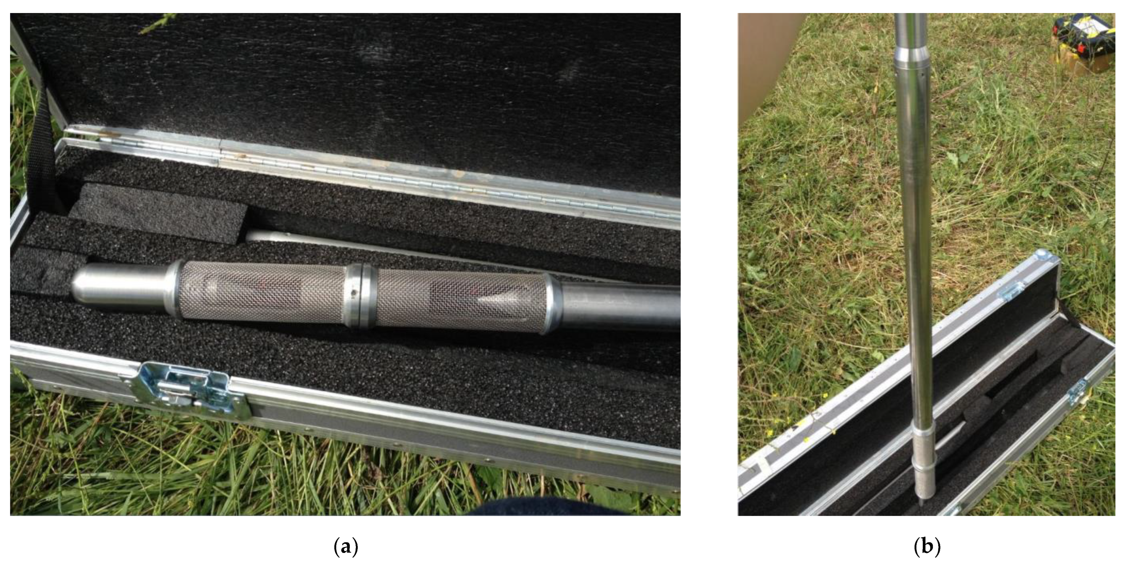
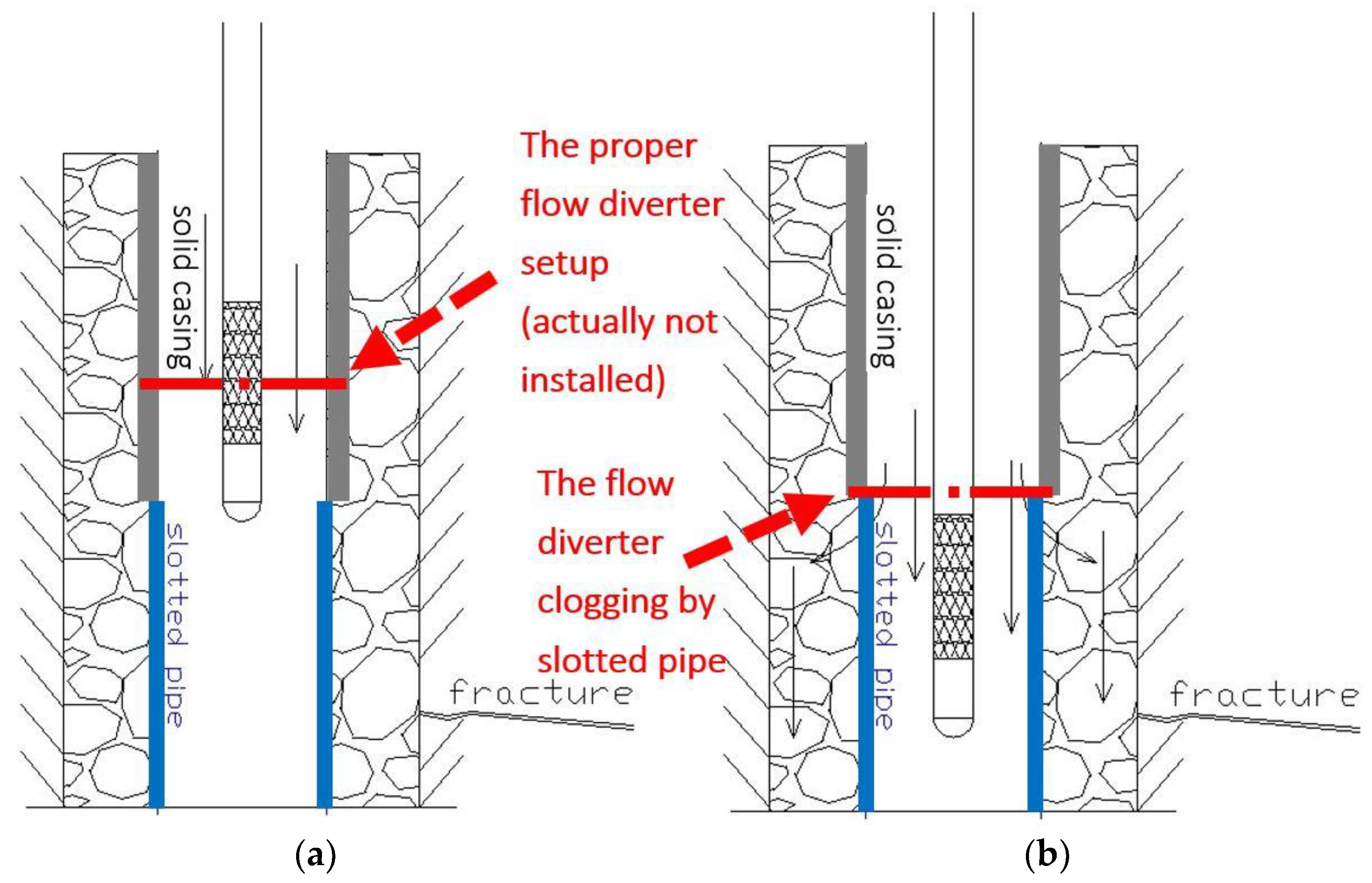
Due to lacking experience in using HPFM, the predrilled borehole was solid-cased by steel and PVC pipes with backfilled gravel. Unfortunately, the diameter of the cased borehole was also smaller than that of the flow diverter (see Figure 6a,b), so the diverter could not be fitted into each borehole, and the in-situ calibration tests had to be done.

(2)

Again, the best testing condition should be with installing the HPFM diverter, as without it, the insufficient flow was diverted into the probe tip, where more water flow could bypass. Thus, the borehole diameter should be carefully prepared to fit the diverter diameter almost perfectly.

(3)

Otherwise, provided that the borehole diameter is much larger than the diverter diameter, not only does more water flow bypass the probe tip, but the borehole will also be more vulnerable to potential borehole collapsing.

(4)

The backfilled gravel tightly contacted with the borehole wall became a segregated section for generating vertical preferential flow paths that alleviate in/outflow around a fracture at its corresponding location but discharged more water downward to supply water circulating at the borehole bottom.

(5)

Based on the aforementioned reflections, no borehole casing seems to provide a perfect testing condition for HPFM; i.e., it is vital to mention the dilemma between the collapsing-induced mud-clogging of the HPFM probe tip (under no borehole casing condition) and the unexpected spurious flow and upward flow at the borehole bottom (under borehole casing condition).

(6)

Moreover, since many studies have reported the success of in-situ flow measurement under borehole casing conditions, there is no completely suitable recommendation regarding this dilemma. Still, other HPFM practitioners must find their best option based on the in-situ geological conditions.

5. Patents

United States of America (USA) Geological Survey originally developed the heat pulse flowmeter (HPFM), and Mount Sopris Instrument Co., Denver, CO, USA, manufactured the HFP-2293. The software of groundwater inversion modelling for borehole flow measurement, FWRAP, was developed, provided and authorised in this work by Prof. Frederick L. Paillet [53].

References

1. Li, L. Multi-Scale, Two-Phase Flow in Complex Coal Seam Systems; Australian Coal Association Research Program (ACARP): Brisbane, Australia, 2011; pp. 7–15. [Google Scholar]
2. Hancock, P.J. Human impacts on the stream–groundwater exchange zone. Environ. Manag. 2002, 29, 763–781. [Google Scholar] [CrossRef]
3. Ma, Y. Preferential Flow Paths in A Complex Coal Seam System. Ph.D. Thesis, University of Queensland, Brisbane, Australia, 2015. [Google Scholar]
4. Ma, Y.; Kong, X.Z.; Zhang, C.; Scheuermann, A.; Bringemeier, D.; Li, L. Quantification of Natural CO2 Emission Through Faults and Fracture Zones in Coal Basins. Geophys. Res. Lett. 2021, 48, e2021GL092693. [Google Scholar] [CrossRef]
5. Busse, J.; Scheuermann, A.; Bringemeier, D.; Hossack, A.; Li, L. In-Situ coal seam and overburden permeability characterization combining downhole flow meter and temperature logs. Contemp. Trends Geosci. 2016, 5, 1–17. [Google Scholar] [CrossRef]
6. Busse, J.; Paillet, F.; Hossack, A.; Bringemeier, D.; Scheuermann, A.; Li, L. Field performance of the heat pulse flow meter: Experiences and recommendations. J. Appl. Geophys. 2016, 126, 158–171. [Google Scholar] [CrossRef]
7. Bear, J. Dynamics of Fluids in Porous Media; American Elsevier Publishing Company, Inc.: New York, NY, USA, 1972. [Google Scholar]
8. Lu, N.; Likos, W.J. Unsaturated Soil Mechanics; John Wiley & Sons: Hoboken, NJ, USA, 2004. [Google Scholar]
9. Fredlund, D.G.; Rahardjo, H. Soil Mechanics for Unsaturated Soils; John Wiley & Sons: Hoboken, NJ, USA, 1993. [Google Scholar]
10. Yan, G.; Li, Z.; Galindo Torres, S.A.; Scheuermann, A.; Li, L. Transient Two-Phase Flow in Porous Media: A Literature Review and Engineering Application in Geotechnics. Geotechnics 2022, 2, 32–90. [Google Scholar] [CrossRef]
11. Freeze, R.A.; Cherry, J.A. Groundwater; Prentice-Hall Inc.: Eaglewood Cliffs, NJ, USA, 1979. [Google Scholar]
12. Fetter, C. Applied Hydrogeology, 4th ed.; Prantice-Hall Inc.: Eaglewood Cliffs, NJ, USA, 2001; p. 621. [Google Scholar]
13. Yan, G.; Ma, Y.; Scheuermann, A.; Li, L. The Hydraulic Properties of Aquabeads Considering Forchheimer Flow and Local Heterogeneity. Geotech. Test. J. 2022, 45, 891–900. [Google Scholar] [CrossRef]
14. ASTM D2434-68; Standard Test Method for Permeability of Granular Soils (Constant Head). ASTM International: West Conshohocken, PA, USA, 2006.
15. ASTM D7664-10; Standard Test Methods for Measurement of Hydraulic Conductivity of Unsaturated Soils. ASTM International: West Conshohocken, PA, USA, 2010.
16. Yan, G.; Bore, T.; Schlaeger, S.; Scheuermann, A.; Li, L. Investigating scale effects in soil water retention curve via spatial time domain reflectometry. J. Hydrol. 2022, 612, 128238. [Google Scholar] [CrossRef]
17. Yan, G.; Bore, T.; Bhuyan, H.; Schlaeger, S.; Scheuermann, A. The Technical Challenges for Applying Unsaturated Soil Sensors to Conduct Laboratory-Scale Seepage Experiments. Sensors 2022, 22, 3724. [Google Scholar] [CrossRef]
18. Li, Z.; Galindo-Torres, S.; Yan, G.; Scheuermann, A.; Li, L. A lattice Boltzmann investigation of steady-state fluid distribution, capillary pressure and relative permeability of a porous medium: Effects of fluid and geometrical properties. Adv. Water Resour. 2018, 116, 153–166. [Google Scholar] [CrossRef]
19. Li, Z.; Galindo-Torres, S.; Yan, G.; Scheuermann, A.; Li, L. Pore-scale simulations of simultaneous steady-state two-phase flow dynamics using a lattice Boltzmann model: Interfacial area, capillary pressure and relative permeability. Transp. Porous Media 2019, 129, 295–320. [Google Scholar] [CrossRef]
20. Yan, G.; Li, Z.; Bore, T.; Torres, S.A.G.; Scheuermann, A.; Li, L. Discovery of Dynamic Two-Phase Flow in Porous Media Using Two-Dimensional Multiphase Lattice Boltzmann Simulation. Energies 2021, 14, 4044. [Google Scholar] [CrossRef]
21. Yan, G.; Li, Z.; Bore, T.; Galindo Torres, S.A.; Scheuermann, A.; Li, L. A lattice Boltzmann exploration of two-phase displacement in 2D porous media under various pressure boundary conditions. J. Rock Mech. Geotech. Eng. 2022, 14, 1782–1798. [Google Scholar] [CrossRef]
22. Darcy, H.; Bazin, H. Recherches Hydrauliques: Recherches Expérimentales sur l’écoulement de l’eau dans les Canaux Découverts. 1ère Partie; Dunod: Pairs, French, 1865; Volume 1. [Google Scholar]
23. Yan, G.; Shi, H.; Ma, Y.; Scheuermann, A.; Li, L. Intrinsic permeabilities of transparent soil under various aqueous environmental conditions. Géotechnique Lett. 2022, 12, 225–231. [Google Scholar] [CrossRef]
24. Singhal, B. Nature of hard rock aquifers: Hydrogeological uncertainties and ambiguities. In Groundwater Dynamics in Hard Rock Aquifers; Springer: Berlin/Heidelberg, Germany, 2008; pp. 20–39. [Google Scholar]
25. Bonnet, E.; Bour, O.; Odling, N.E.; Davy, P.; Main, I.; Cowie, P.; Berkowitz, B. Scaling of fracture systems in geological media. Rev. Geophys. 2001, 39, 347–383. [Google Scholar] [CrossRef]
26. Clarkson, C.R.; Bustin, R. Coalbed methane: Current field-based evaluation methods. SPE Reserv. Eval. Eng. 2011, 14, 60–75. [Google Scholar] [CrossRef]
27. Dron, R. Notes on cleat in the Scottish coalfield. Trans. Inst. Min. Metall. 1925, 70, 115–117. [Google Scholar]
28. Tsang, C.F.; Neretnieks, I. Flow channeling in heterogeneous fractured rocks. Rev. Geophys. 1998, 36, 275–298. [Google Scholar] [CrossRef]
29. Massarotto, P.; Rudolph, V.; Golding, S.; Wang, F.; Iyer, R. Scaleup of laboratory measured coal permeability. In Proceedings of the 2008 Asia Pacific Coalbed Methane Symposium, Brisbane, Australia, 22–24 September 2008. [Google Scholar]
30. DeAngelis, D.L.; Yeh, G.; Huff, D. Integrated Compartmental Model for Describing The Transport of Solute in a Fractured Porous Medium; Oak Ridge National Lab.: Oak Ridge, TN, USA, 1984.
31. Legrand, H. Evaluation techniques of fractured-rock hydrology. In Developments in Water Science; Elsevier: Amsterdam, The Netherlands, 1979; Volume 12, pp. 333–346. [Google Scholar]
32. Neuville, A.; Toussaint, R.; Schmittbuhl, J. Hydrothermal coupling in a self-affine rough fracture. Phys. Rev. E 2010, 82, 036317. [Google Scholar] [CrossRef]
33. Kirsch, R. Groundwater Geophysics: A Tool for Hydrogeology; Springer: Berlin/Heidelberg, Germany, 2006. [Google Scholar]
34. Price, D.G. Engineering Geology: Principles and Practice; Springer Science & Business Media: Berlin/Heidelberg, Germany, 2008. [Google Scholar]
35. Elci, A.; Molz, F.J., III; Waldrop, W.R. Implications of observed and simulated ambient flow in monitoring wells. Groundwater 2001, 39, 853–862. [Google Scholar] [CrossRef]
36. Mayo, A.L. Ambient well-bore mixing, aquifer cross-contamination, pumping stress, and water quality from long-screened wells: What is sampled and what is not? Hydrogeol. J. 2010, 18, 823. [Google Scholar] [CrossRef]
37. Izbicki, J.A.; Teague, N.F.; Hatzinger, P.B.; Böhlke, J.K.; Sturchio, N.C. Groundwater movement, recharge, and perchlorate occurrence in a faulted alluvial aquifer in California (USA). Hydrogeol. J. 2015, 23, 467. [Google Scholar] [CrossRef]
38. Poulsen, D.L.; Cook, P.G.; Simmons, C.T.; McCallum, J.L.; Dogramaci, S. Effects of intraborehole flow on purging and sampling long-screened or open wells. Groundwater 2019, 57, 269–278. [Google Scholar] [CrossRef]
39. Poulsen, D.L.; Cook, P.G.; Simmons, C.T.; Solomon, D.K.; Dogramaci, S. Depth-Resolved Groundwater Chemistry by Longitudinal Sampling of Ambient and Pumped Flows within Long-Screened and Open Borehole Wells. Water Resour. Res. 2019, 55, 9417–9435. [Google Scholar] [CrossRef]
40. Huang, Y.; Li, Y.; Knappett, P.S.; Montiel, D.; Wang, J.; Aviles, M.; Hernandez, H.; Mendoza-Sanchez, I.; Loza-Aguirre, I. Water quality assessment bias associated with long-screened wells screened across aquifers with high nitrate and arsenic concentrations. Int. J. Environ. Res. Public Health 2022, 19, 9907. [Google Scholar] [CrossRef]
41. Molz, F.; Boman, G.; Young, S.; Waldrop, W. Borehole flowmeters: Field application and data analysis. J. Hydrol. 1994, 163, 347–371. [Google Scholar] [CrossRef]
42. Pitrak, M.; Mares, S.; Kobr, M. A simple borehole dilution technique in measuring horizontal ground water flow. Groundwater 2007, 45, 89–92. [Google Scholar] [CrossRef]
43. Monier-Williams, M.; Davis, R.; Paillet, F.; Turpening, R.; Sol, S.; Schneider, G. Review of Borehole Based Geophysical Site Evaluation Tools and Techniques; Nuclear Waste Management Organization: Toronto, ON, Canada, 2009. [Google Scholar]
44. Hess, A.E. Identifying hydraulically conductive fractures with a slow-velocity borehole flowmeter. Can. Geotech. J. 1986, 23, 69–78. [Google Scholar] [CrossRef]
45. Paillet, F.L.; Hess, A.; Cheng, C.; Hardin, E. Characterization of fracture permeability with high-resolution vertical flow measurements during borehole pumping. Groundwater 1987, 25, 28–40. [Google Scholar] [CrossRef]
46. Pehme, P.E.; Greenhouse, J.P.; Parker, B.L. The active line source temperature logging technique and its application in fractured rock hydrogeology. J. Environ. Eng. Geophys. 2007, 12, 307–322. [Google Scholar] [CrossRef]
47. Paillet, F.L. Flow modeling and permeability estimation using borehole flow logs in heterogeneous fractured formations. Water Resour. Res. 1998, 34, 997–1010. [Google Scholar] [CrossRef]
48. Paillet, F.; Hite, L.; Carlson, M. Integrating surface and borehole geophysics in ground water studies—An example using electromagnetic soundings in south Florida. J. Environ. Eng. Geophys. 1999, 4, 45–55. [Google Scholar] [CrossRef]
49. Paillet, F.L. A field technique for estimating aquifer parameters using flow log data. Groundwater 2000, 38, 510–521. [Google Scholar] [CrossRef]
50. Paillet, F.L. Borehole flowmeter applications in irregular and large-diameter boreholes. J. Appl. Geophys. 2004, 55, 39–59. [Google Scholar] [CrossRef]
51. Mount Sopris Instruments, Co. Mannual of HFP-2293—Heat Pulse Flowmeter. Mount Sopris Instruments Co.: Denver, CO, USA, 2002. [Google Scholar]
52. Molz, F.J.; Morin, R.H.; Hess, A.E.; Melville, J.G.; Güven, O. The impeller meter for measuring aquifer permeability variations: Evaluation and comparison with other tests. Water Resour. Res. 1989, 25, 1677–1683. [Google Scholar] [CrossRef]
53. Paillet, F. FWRAP; U.S. Geological Survery: Denver, CO, USA, 2012.
54. Cooper, H.H., Jr.; Bredehoeft, J.D.; Papadopulos, I.S. Response of a finite-diameter well to an instantaneous charge of water. Water Resour. Res. 1967, 3, 263–269. [Google Scholar] [CrossRef]
55. Davis, S.N.; De Wiest, R.J. Hydrogeology; Wiley: New York, NY, USA, 1966; Volume 463. [Google Scholar]
56. Coal & Allied Operations Pty Ltd. Hunter Valley Operations South Coal Project: Environmental Assessment Report Volume I; Coal & Allied Operations Pty Ltd.: Sydney, Australia, 2008; pp. 1–1224. [Google Scholar]
57. Age Australasian Groundwater & Environmental Consultants Pty Ltd. 2011 Hunter Valley Operation (HVO) Carrington Groundwater Impacts Report; Australian Coal Association Research Program (ACARP): Brisbane, Australia, 2012. [Google Scholar]
58. Williams, J.; Paillet, F.L. Using flowmeter pulse tests to define hydraulic connections in the subsurface: A fractured shale example. J. Hydrol. 2002, 265, 100–117. [Google Scholar] [CrossRef]
Figure 1. The HPFM probe (HFP-2293, manufactured by Mount Sopris Instrument Co., Denver, CO, USA): (a) The horizontal zoom-in of the HPFM probe tip (the heat grid wire in between two thermistor sensors and the signal-sending/detecting region covered by a fine-mesh grid to block floating coarse in boreholes) and (b) The vertical overview of HFP-2293, including the probe tip and the main probe body in the overall length of 120 cm (the distance between the probe tip and the heat grid is 20 cm).
Geosciences 13 00146 g001
Figure 2. An illustration of the HPFM probe in-situ installation in the field: (a) The borehole, tripod and pulley (lower the HPFM probe into each borehole by a cable connected to a winch); (b) The overview of the working environment (the software will receive the signal through the surface monitoring equipment to either start or record a flow rate measurement); (c) A typical flow rate display in the appending software of HFP-2293: MatrixHeat [51] (signal peak; the x-axis represents the time, and the y-axis represents the temperature) and (d) An unclear flow rate display in MatrixHeat (multiple peaks exist, so it is mandatory to correctly pick up the single peak point for a flow rate analysis).
Geosciences 13 00146 g002
Figure 3. A scatter chart of an in-situ flow rate profile of borehole A435_R_056 (Trip 2) (the upward flow in positive value and the downward flow in negative value).
Geosciences 13 00146 g003
Figure 4. The operating interface of FWRAP.
Geosciences 13 00146 g004
Figure 5. Hunter Valley Operations (HVO) in Hunter Valley, New South Wales, Australia: (a) The location of HVO in the northwest of Newcastle, NSW, Australia; (b) The map of an overview of HVO; (c) The zoom-in of HVO’s mining extension zone before open-cut mining operation and (d) The schematic diagram of transect A–B for a demonstration of HVO open-cut mining adversely impacting on the adjacent groundwater system and surface water in Hunter River nearby (the solid black lines show the fractures and faults structure in the rock).
Geosciences 13 00146 g005aGeosciences 13 00146 g005b
Figure 6. The challenges of the in-situ HPFM setup in the HVO mining extension zone: (a) A schematic sketch of the in-situ borehole casing approach for the steel pipe (in 15–24 m depth, highlighted in grey colour) and (b) A schematic sketch of the in-situ borehole casing approach for the slotted PVC pipe (below 24 m, highlighted in blue colour).
Geosciences 13 00146 g006
Figure 7. The selected drilling locations of boreholes in the mining extension zone of HVO (see Figure 5c): (a) the field trip of October 2012 and (b) the field trip of April 2013.
Geosciences 13 00146 g007
Figure 8. In-situ flow logging and the analysed flow rate profile for the borehole: A435_R_045 (Trip 2) (the upward flow in positive value and the downward flow in negative value).
Geosciences 13 00146 g008
Figure 9. In-situ flow logging and the analysed flow rate profile for the borehole: A435_R_056 (the upward flow in positive value and the downward flow in negative value).
Geosciences 13 00146 g009
Figure 10. The comparison between (a) other GI methods (e.g., the in-situ electrical resistance (resist SP), gamma ray, calliper and density logging) for the borehole: A435_R_056 (the upward flow in positive value and the downward flow in negative value) and (b) the flow rate profile (datasets and fitted one).
Geosciences 13 00146 g010
Figure 11. In-situ flow logging and the analysed flow rate profile for the borehole: A435_R_059 (the upward flow in positive value and the downward flow in negative value).
Geosciences 13 00146 g011
Figure 12. The comparison between (a) other GI methods (e.g., in-situ electrical resistance (resistance SP), gamma ray, calliper and density logging) for the borehole: A435_R_059 (the upward flow in positive value and the downward flow in negative value) and (b) the flow rate profile (datasets and fitted one).
Geosciences 13 00146 g012
Figure 13. Comparison between unanalysable and analysable datasets for the same borehole in two field trips: (a) A435_R_045 (Trip 1) and (b) A435_R_045 (Trip 2) (the upward flow in positive value and the downward flow in negative value).
Geosciences 13 00146 g013
Figure 14. The demonstrations of totally unanalysable datasets: (a) A435_C_003; (b) A435_R_043; (c) A435_R_049; (d) A435_R_054; (e) A435_R_040; (f) A435_R_046 and (g) A435_R_050 (the upward flow in positive value and the downward flow in negative value).
Geosciences 13 00146 g014aGeosciences 13 00146 g014b
Figure 15. The demonstration of partially unanalysable or analysable datasets (A435_R_060) (the upward flow in positive value and the downward flow in negative value).
Geosciences 13 00146 g015
Figure 16. The demonstrations of totally analysable datasets with measurement errors: (a) A435_R_042; (b) A435_R_044; (c) A435_R_051 (Trip 1) and (d) A435_R_051 (Trip 2) (the upward flow in positive value and the downward flow in negative value) (flow rates reach zero at borehole bottom).
Geosciences 13 00146 g016