1. Introduction
Mauna Kuwale is a mass of icelandite and rhyodacite lying between flows of basalt. Ryodacite is fine-grained igneous rock that forms from rapid cooling of lava with a composition between dacite and rhyolite. It is relatively rich in silica with low content in metal oxides. Icelandite is a Fe-rich volcanic rock with a composition between rhyodacite and tholeiitic basalt with a content in SiO2 which is typically greater than 60%.
The first K-Ar age dating indicated that the Mauna Kuwale rhyodacite is several million years older than the nearby basalts and on that basis, it was suggested that the rhyodacite was part of an earlier volcano buried by the Wai’anae volcanics. The volcanic mass appears to be a short thick flow, or possibly a flow, interbedded with the caldera-filling [
1] lavas of the Wai’anae volcano. This formation is probably the oldest root of a volcano on the Pacific plate (i.e., [
1]).
It is known that the AMS of volcanic rocks (e.g., basalts) is very weak but it has been used very successfully to differentiate between magmatic in origin or tectonically deformed structure, our previous study of dikes emplaced in the Wia’anae volcano indicate that such basaltic bodies have been unaffected by tectonic deformation (e.g., [
2,
3,
4,
5]) and have shown a purely magmatic behavior in origin. The AMS technique works relatively well and can be used advantageously to investigate the fabric of magnetic minerals in rocks by means of the determination of direction of flow using magnetic susceptibility parameters of an ellipsoid with three orthogonal axes that correspond to the maximum (K
1), intermediate (K
2) and minimum principal axes (K
3) (e.g., [
6,
7]). In reality, AMS is the only method that yields justifiable and plausible results in rocks such as basalts with very weak preferred orientation of mineral (i.e., magnetic minerals in general). In undeformed volcanic rocks the AMS technique has been interpreted to reflect the preferred orientation of titanomagnetite grains by grain shape produced by the lava flow (e.g., [
7,
8,
9,
10]). As a result the obtained magnetic fabric is therefore conformable to the shapes of the volcanic bodies under question. Furthermore, it has been demonstrated that in lava flows, sills, and other tabular bodies, the magnetic foliation is approximately parallel to the dominant plane and the magnetic lineation is often parallel to the flow direction even though it can also be perpendicular (for summary see [
7,
11]).
Thus far, we know that magnetic anisotropy is among the most important techniques in rock fabric analysis because it can be used to indirectly and efficiently investigate the preferred orientation of magnetic minerals in rocks, i.e., the magnetic fabric. The goal of our magnetic mineralogy properties and AMS petrofabric study is to investigate and test the hypothesis that the Icenlandite and Rhyodacite flows and their respective colling units, have not been affected by tectonic deformation or are characterized by strictly magmatic origin once we determine their predominant direction of flow of the lavas in question and have a good understanding of the mineral properties and their relation to their petrofabrics
We present the first magnetic study of the Mauna Kuwale flows of Wai’anae Volcano, O’ahu, Hawaii. We have undertaken a rock magnetic characterization including magnetic susceptibility, and anisotropy of magnetic susceptibility (AMS), as well as high field characterization with hysteresis, magnetic granulometry and IRM measurements. Magnetic mineralogy was also evaluated with the analysis of magnetic susceptibility dependence with temperature.
2. Geologic Setting
The pioneering and seminal work of [
12,
13,
14], produced the most complete and accurate description of the Islands of Hawaii. Even though originally such geologic document meant to be for the search of ground-water resources of the islands, specific for O’ahu. Even today, such results prevail in terms of the knowledge of the geology and other natural resources.
O’ahu volcanic structure consists of the remnants of two eroded lava shield volcanoes, Wai’anae and Ko’olau.
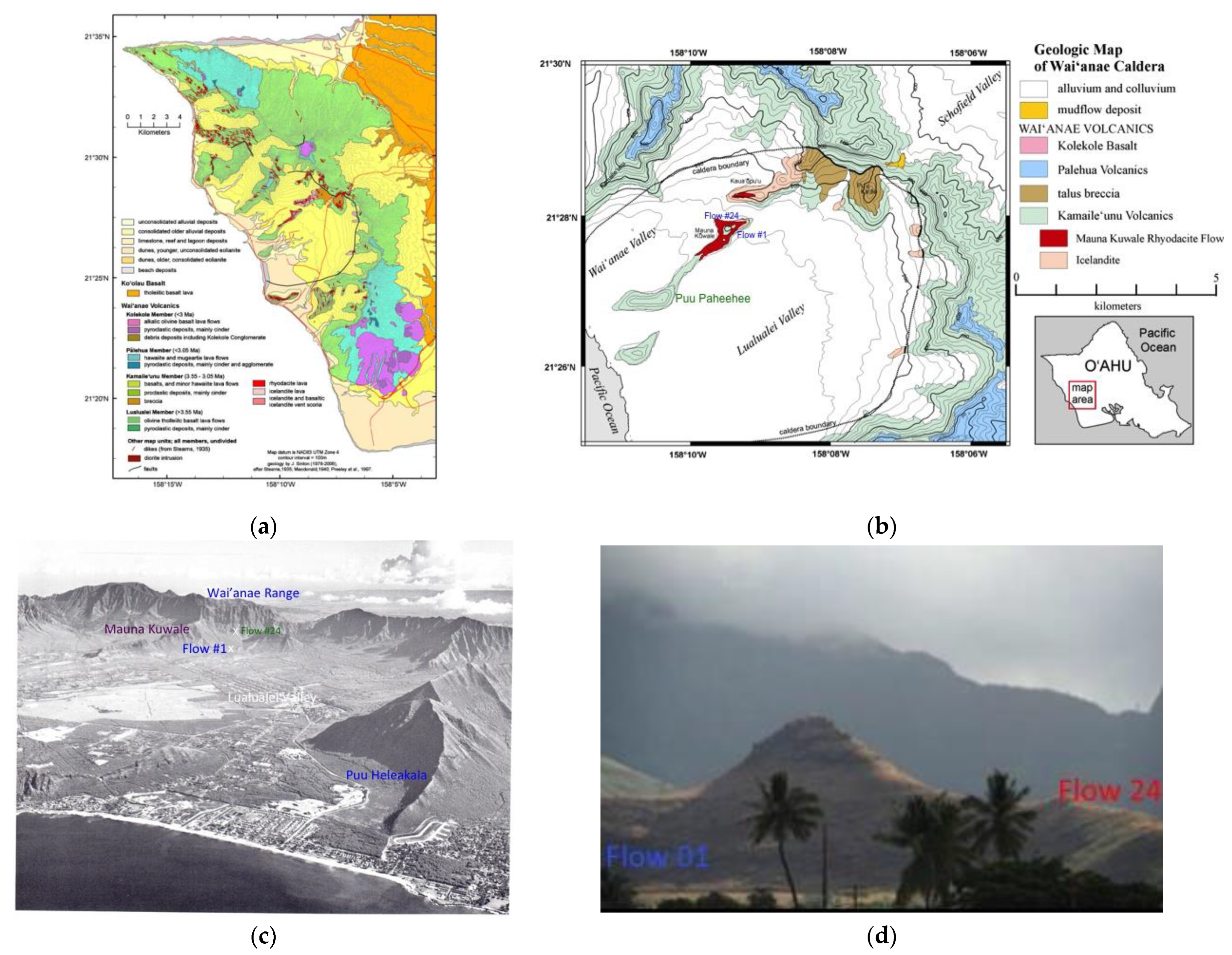
The Wai’anae volcano, that rises up to 1227 m above sea level at Mount Ka’ala, (see
Figure 1) has been mapped by [
15,
16] using geochemical as well as structural and lithologic criteria to define map units. It consists of a tholeiitic shield with thick cap of transitional to alkalic rocks [
16,
17]. Rejuvenation stage volcanics of undetermined age occurs at Kolekole Pass and forms a line of well-preserved cinder cones on the southern flank of the Wai’anae volcano. Wai’anae is very deeply eroded and Lualualei and Wai’anae valleys present a landscape that is unusual for Hawai’i, in which, narrow and nearly vertical-sided ridges, some of them isolated, rise abruptly from the flat valley floors [
15,
17,
18].
The Wai’anae volcano can be divided into two formations, the Wai’anae volcanics and the Kolekole volcanics [
12,
13,
14,
15].
The Kolekole volcanics consist of a series of cinder cones and short flows of mafic alkalic composition; they are the youngest eruptive products of the volcano.
The Wai’anae volcanics were emplaced during the main active phase of the volcano and include both tholeiitic and alkalic magmas. It has been formally subdivided into the Lualualei Member (oldest 3.8–3.5 Ma), Kamai’leunu Member (3.5–3.2 Ma), and Palehua Member (3.2–2.9 Ma) (e.g., [
15,
16]). The latter corresponds to the post-shield “alkalic cap” of the Wai’anae volcano and is composed of alkalic hawaiites and rarer mugearites
According to [
16] the Kamai’leunu Member includes a formally named flow, the Mauna Kuwale Rhyodacite Flow. The eruptive center was approximately where Pu’u Kailio is now; flows dip at angles of up to 15° away from this hill [
15]. Dips of Kamai’leunu Member flows are gentler than those of Lualualei flows. The eruptive center was at about the same place as that of the Lualualei Member. A typical Kamai’leunu flow is thicker and has a higher proportion of aa than its Lualualei counterpart [
20]. The Kolekole volcanics, which are also of formational rank, are geographically extended to include certain cones and flows previously included in the upper member of the Wai’anae volcanic series by, e.g., [
12,
18].
As pointed out by the different researchers who have studied the paleomagnetism and petrofabrics (e.g., [
5,
21,
22]) and the volcanic stratigraphy and dating of the Wai’anae volcanics, the average extrusion rate of the lavas is one flow every 500 to 1400 years, with flows thickness averaging 2 m. The period of 500 to 1400 years is such good agreement with the estimate of [
23] that 1000 years may be a realistic figure for the average time between superimposed flows of Mauna Loa and Kilauea and indicate further that Hawaiian shield volcanoes were built rapidly.
The lava at Mauna Kuwale with 66 wt% SiO
2 was initially referred by [
18,
24] as a rhyodacite. These lavas are exposed as intracaldera dikes and flows, and constitute the only known silicic, icelandite and rhyodacite lavas lying between flows of basalt of the Hawaiian chain.
Rhyodacite is fine-grained igneous rock that forms from rapid cooling of lava with a composition between dacite and rhyolite. It is relatively rich in silica with low content in metal oxides. It may present variable percentages of quartz, between 20% and 60%, with plagioclase making near two-thirds of the total feldspar content. The content in SiO
2 is typically between 69% and 72% by weight. The Mauna Kuwale Rhyodacite flow is now a formally accepted stratigraphic unit of the Wai‘anae Volcano [
16]. Icelandite is a Fe-rich volcanic rock with a composition between rhyodacite and the tholeiitic basalt with a content in SiO
2 is typically greater than 60%. Rhyodacite magma was derived from a basaltic parent [
25].
The Mauna Kuwale section has basalts and basaltic icelandites at the base, overlain by the flows of hornblende-biotite-hypersthene rhyodacite formed by melting of the lower crust. The contact between the icelandites and rhyodacites is not well-defined showing interlayering.
This sequence is overlain, unconformably, by plagioclase-phyric pahoehoe basalts, and mildly alkalic, plagioclase-rich basaltic hawaiites, that form the capping peak of Mauna Kūwale.
The topmost icelandite flow is about 62 m thick and is overlain by the Mauna Kuwale rhyodacite flow, with a maximum thickness of ≈ 90 m [
26].
According to [
27] the Mauna Kuwale Rhyodacite erupted near the beginning of the Mammoth reversely polarized event within the Gauss Chron, indicating an age of 3.3 Ma. [
27] refer that “plagioclase phenocrysts of the rhyodacite rock show intense forms of sieve texture, commonly with a zone of glass blebs between the crystalline core and rim”.
4. Magnetic Susceptibility, Anisotropy and Magnetic Fabric
The fundamentals of magnetic susceptibility and anisotropy are extensively described in several textbooks and articles (e.g., [
6,
9,
28]). Anisotropy of magnetic susceptibility (AMS) of a rock is mathematically represented by a second rank tensor k and can be represented geometrically by an ellipsoid of magnetic susceptibility. Following this approach, k is described by three different eigenvectors, that define three orthogonal axes of the ellipsoid of the susceptibility. These axes are designated as maximum, intermediate, and minimum susceptibilities may be represented as k
1 > k
2 > k
3, respectively. These axes define a ellipsoid of AMS which shape may vary between a flattened (or oblate) shape to an elongated (or prolate) shape. Intermediate shapes are designated as triaxial.
The principal susceptibilities k
1, k
2 and k
3 and their relationship are used to define shape parameters that are combinations of magnitude parameters. Most common parameters are the bulk susceptibility K = (k
1 + k
2 + k
3)/3, the degree of magnetic lineation L = (k
1 − k
2)/K, the degree of magnetic foliation L = (k
2 − k
3)/K. The morphology of the AMS ellipsoid was analyzed by the distribution of the AMS axes through the AGICO Anisoft-5.1.08. magnetic anisotropy data analysis program [
29] with the mean tensors and principal directions k
1, k
2 and k
3, under the 95% confidence ellipses, calculated by the [
30] statistics.
The shape parameter, T [
31] is defined as T = (2η
2 − η
1 − η
3)/(η
1 − η
3), where η
1 = ln k
1, η
2 = ln k
2, and η
3 = ln k
3. A positive T value means that the shape of the AMS ellipsoid of the specimen is characterized by an oblate geometry while a negative T value indicates prolate shape [
6].
The degree of anisotropy of the ellipsoid of susceptibility, referred as P’ = exp [2((ln (k
1/K))
2 + (ln (k
2/K))
2 + (ln (k
3/K))
2)]
1/2. AMS may also be expressed as percentage in the form: P% = 100% × (k
1 − k
3)/K [
31].
5. Analytic Procedures, Magnetic Measurements
The magnetic susceptibility and its anisotropy were measured with a MFK1-FA Multi-Function Kappabridge (Agico) operating at a low field of 200 A/m and frequency of 976 Hz using an AGICO standard specimen holder (15 rotation positions). The measurements performed in the Petrofabrics and Paleomagnetics Laboratory of the HIGP- SOEST, University of Hawaii and Paleomagnetic Laboratory of the Instituto Dom Luiz (IDL), Lisbon, Portugal. The measurements included all 25 cooling units with, in average, 8 samples per flow.
The k-T experiments were run in a CS4 furnace coupled to a MFK1-FA Multi-Function Kappabridge in the Paleomagnetic Laboratory of IDL, operating at a field of 200 A/m and frequency of 976 Hz. The susceptibility was measured from room temperature up to a maximum of 640 °C with heating and cooling rate of 9 °C/min, under a continuous flowing Ar atmosphere. The measurements were made using 9 specimens to identify the main magnetic phases.
To determine hysteresis parameters such as saturation remanence Magnetization (Mrs), saturation magnetization (Ms), coercive remanence force (Hcr) and coercive force (Hc) and magnetic grain sizes the hysteresis loop measurements were performed on a variable field translation balance (VFTB) with a measuring range of 10−8 to 10−2 A/m of the Petrofabrics and Paleomagnetics Laboratory of the HIGP- SOEST, University of Hawaii. The maximum field applied was 1 Tesla and a high-field paramagnetics corrections was applied by means of a software provided by the manufacturer of the VFTB instrument. For each of the 25 cooling units powder samples of approximately 200 mg of 1 representative specimen per flow were prepared.
Uniaxial isothermal remanent magnetization (IRM) and saturation of IRM, (SIRM) were measured in 8 representative specimens. Magnetization was induced with an ASC Scientific IM-10–30 Pulse Magnetizer and the remanent magnetization was measured with an AGICO JR-6 Spinner at the Paleomagnetic Laboratory of IDL. Each specimen was first demagnetized by an alternating magnetic field up to 100 mT and then submitted to a progressive uniaxial increasing DC magnetic field up to 1.1 T. After saturation of magnetization a stepwise demagnetization in backfield was applied until the removal of the IRM to obtain the coercivity of the remanence.
6. Results
6.1. Magnetic Susceptibility and Anisotropy
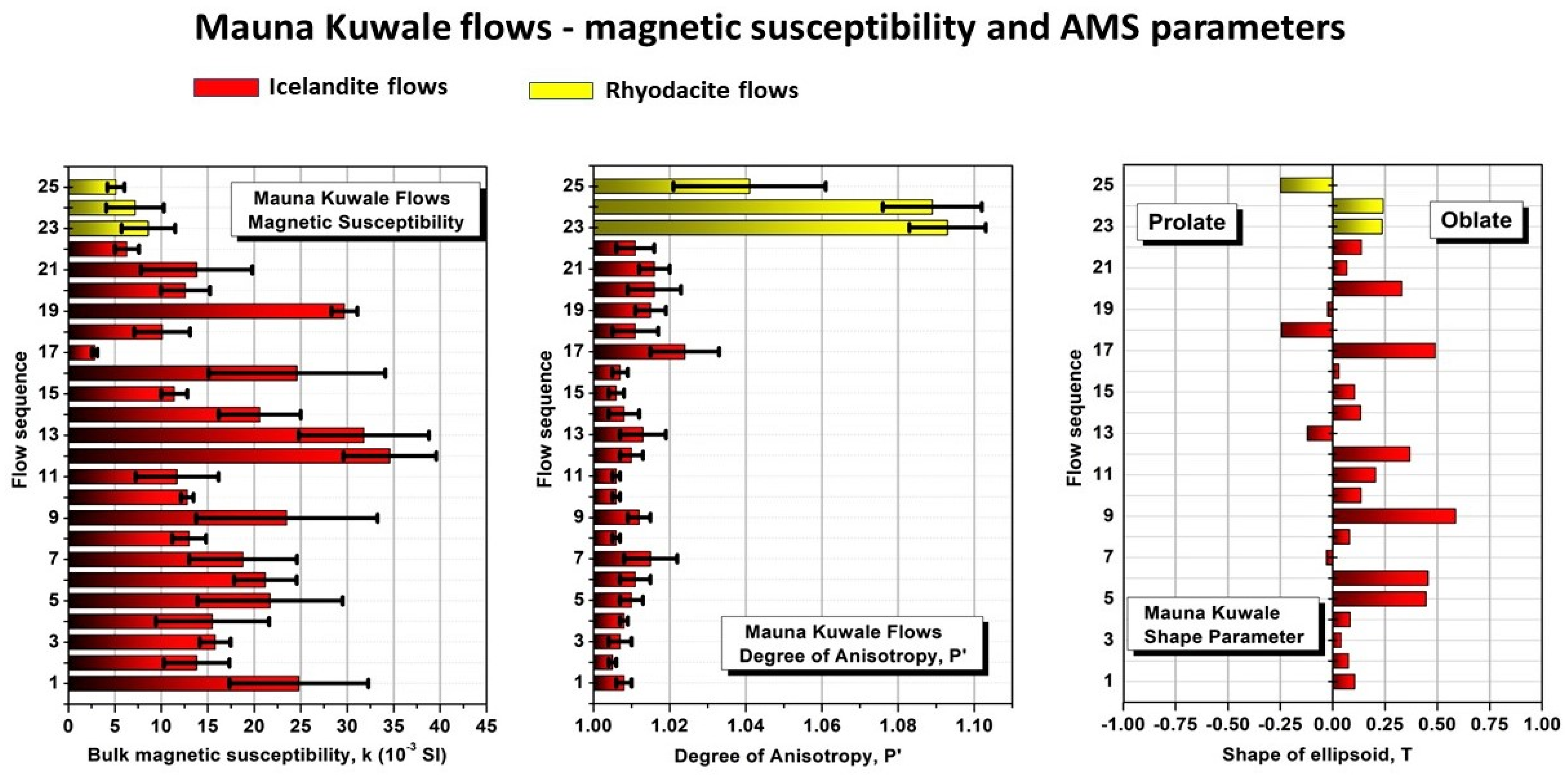
Overall, the bulk magnetic susceptibility (MS) measured in the MK flows is relatively low (
Figure 2 left). Nevertheless, it is possible to identify two groups of MS values: a first group up to cooling unit 21, the MS show an average value of K = 18.3 × 10
−3 SI. Some flows show MS > 30 × 10
−3 SI, and only one flow shows very low MS < 4 × 10
−3 SI. The uppermost 4 cooling units (22 to 25) fall in a 2nd group and show systematically very low MS with a mean value of 6.8 × 10
−3 SI.
The magnetic anisotropy (
Figure 2 center), characterized by the P’ parameter, in most cases is very low, but shows two distinct group of values, almost coincident with the previous defined groups of MS. In general P’ is very low on all cooling units from 1 to 22 with a mean degree of anisotropy P’ < 1.010 but increase markedly in late cooling units 23, 24 and 25 with P’ ranging between 1.040 to 1.090.
The shape of the AMS ellipsoid (
Figure 2 right) is mostly oblate to neutral with just 3 cooling units showing a predominant prolate shape, two icelandite cooling units (13 and 18) and the uppermost rhyodacite flow (i.e., 25). This cooling unit also shows the lowest anisotropy of the rhyodacite cooling units (even so, much higher than the icelandite cooling units).
There is no direct relationship between the shape of ellipsoid and the anisotropy or the magnetic fabric as these prolate shape of ellipsoid occur for high scatter (flow 13) and tri-axial (flows 18 and 25) magnetic fabrics. The prevailing oblate shape indicates, in general, the compaction effect due to the flow emplacement.
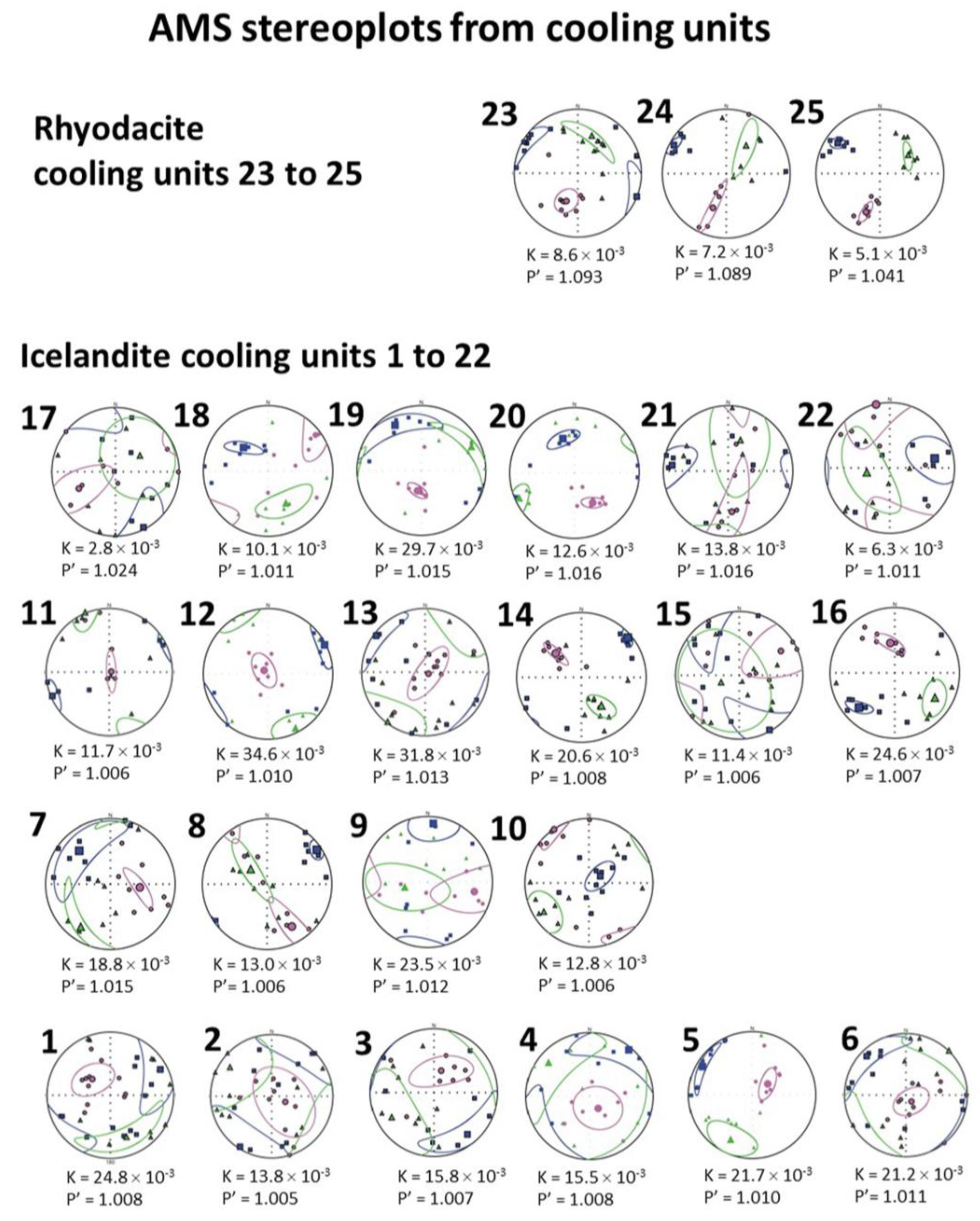
The magnetic fabric (
Figure 3) is in most of the flows, is characterized by vertical to sub-vertical k
3 axis and by sub-horizontal magnetic foliation, defining the normal magnetic fabric in a horizontal or sub-horizontal flow. Despite differences in the shape of ellipsoid (oblate in flow 6 and triaxial in flows 11 and 13) and occasionally showing high scatter of axes (flow 2), the confidence areas of the AMS axes are mostly well constrained, showing a high degree of concentration of axes. Thus, direction of the magnetic lineation is mainly through northern (NE to NW) sectors in the flows.
Magnetic fabric of flows 17 and uppermost flows, 23, 24 and 25, shows that k3 axes are typically oblique, dipping around 45° in a very steady orientation through SW to SSW. On these flows, the magnetic lineation is very steady presenting an azimuth WNW nearly subhorizontal. Interestingly, these cooling units show high values of magnetic anisotropy, especially in cooling units 23 to 25). Cooling unit 17, with a value of P’= 1.024, shows the highest value of anisotropy among all the icelandite cooling units.
From cooling units 1 to 6 despite the high dispersion of magnetic axes the magnetic foliation plane is relatively well defined, broadly sub-horizontal. These cooling units show high MS and low anisotropy. Flows 7 to 10 k3 is mostly oblique to horizontal and fabrics oblate and prolate occur. Flows 11 to 16 show magnetic fabric mostly tri-axial except for one flow (15) with high dispersion.
Cooling units 17 to 22 show usually high dispersion of magnetic axes and k3 axis occur in different orientations. Only two cooling units (19 and 20) show analogous fabric orientation with k3 oblique, for south. Cooling units 23 to 25 of rhyodacite rock show lineation well defined and oriented NW, sub-horizontal. Despite the different oblate to prolate and tri-axial magnetic fabrics observed in each flow, the orientation of the principal directions in these flows is identical.
6.2. Thermo-Magnetic Analysis
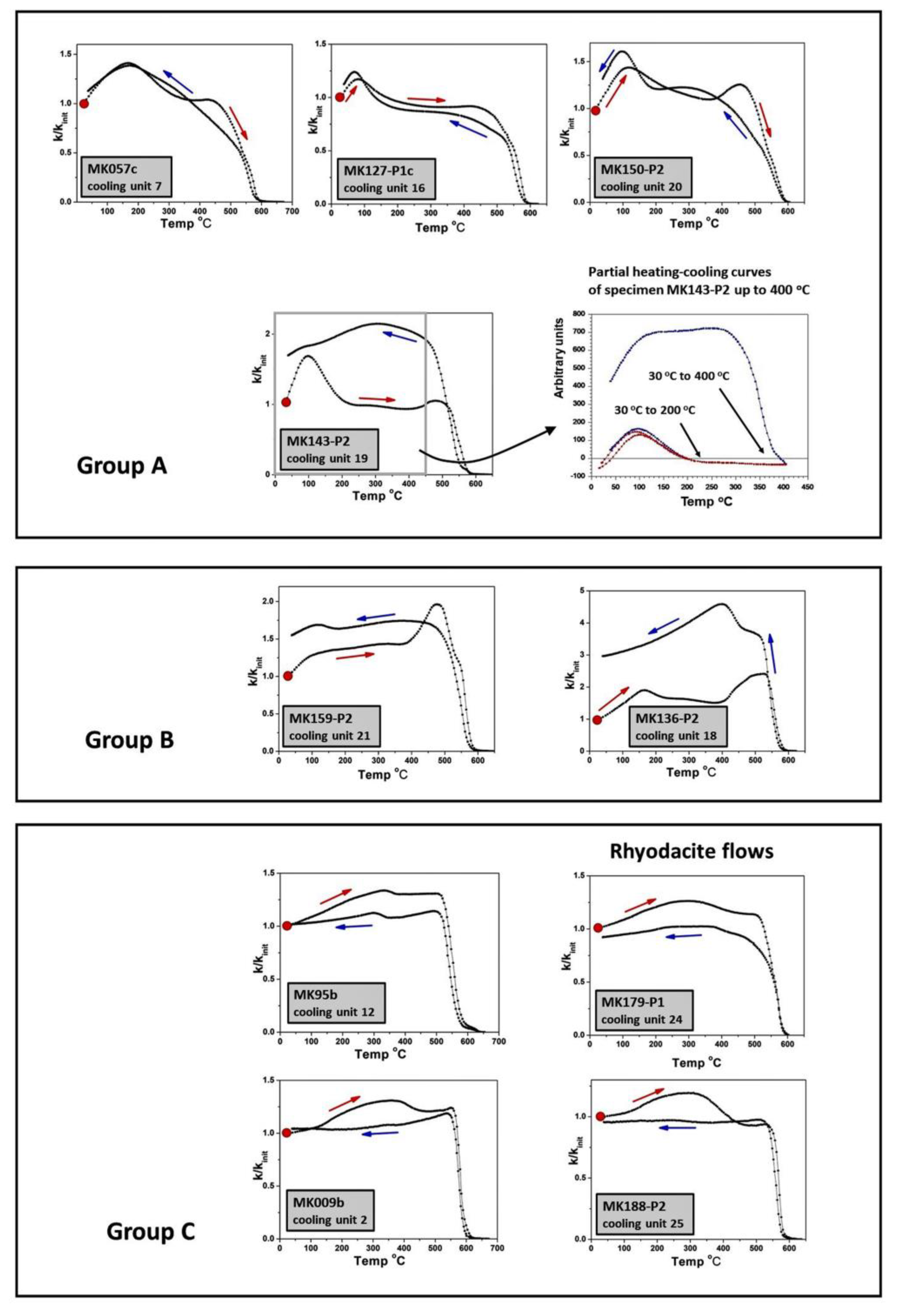
Overall, the samples show irreversible heating/cooling susceptibility curves. The susceptibility of the specimens at room temperature after the cooling phase (one full cycle) is usually equal or slightly higher that the initial susceptibility before heating. As a first approach, it is possible to systematize the thermomagnetic behavior in a sort of transitional group A−B and a distinct group C (
Figure 4).
One group of specimens show a continuous increase of MS until 100–150 °C followed by a drop of the susceptibility, identifying a phase of low Curie temperature. In some specimens this increase of MS and subsequent drop is fast and well-defined as observed in specimens MK127 (cooling unit 16), MK143 (cooling unit 19), MK150 (cooling unit 20).
After a peak or a clear increase in MS about 500 °C, interpreted as a -“Hopkinson peak”-, a final drop of MS reveals a Curie point near 580–590 °C indicating the presence of a magnetite-like phase. After 590 °C the MS vanishes nearly completely.
The cooling curve is roughly reversible specially from 500 °C down to room temperature, It shows clearly the low temperature magnetic phase and the final magnetic susceptibility is nearly equal or slightly higher than initial MS.
A little bit different, the sample MK136-P2 also shows the low temperature magnetic phase and a final phase defined by a Curie temperature of 580–585 °C, but more magnetic mineral is produced in the process and the final MS at room temperature is 3 × the initial MS. These specimens are included in a Group A and are characterized as Titano rich magnetite as well as magnetite.
A different behavior of the K-T curve is observed in samples that we include in Group B, as MK136 (cooling unit 18), MK159 (cooling unit 21), MK164 (cooling unit 22). In these samples it is observed a continuous but slight increase of MS up to 300–350 °C. This peak, that attains it maximum by 500 °C is followed by a fast drop of MS that vanishes at 580–590 °C. This peak is interpreted as a Hopkinson peak suggesting a magnetite phase of single domain size.
The cooling path of the MS is coincident with the heating path only in the interval 580–500 °C. The MS during the cooling path is higher that the observed in the heating path and the final MS at room temperature is higher than the initial MS. The magnetic mineralogy is characterized by Ti-poor titanomagnetite and magnetite.
In samples of both groups, the partial thermo-magnetic curves (see specimen MK143) show a coincident path of the MS between the heating and cooling curves up to ≈ 200 °C which confirms that the low Curie temperature component is primary and not formed by the heating process. Approaching the high temperatures, the non-reversibility or non-coincidence of both paths confirms the formation of a new magnetic phase with a Curie temperature, characteristic of magnetite. The differences in Curie temperatures observed in the last phase (drop of susceptibility) that range between 570–585 °C may be related to variable Ti contents in the titanomagnetite solid solution.
It is important to point out that for samples of Group B there is no drop or a strong decrease of susceptibility in the 100–150 °C, in contrast to what is observed in typical samples of Group A, but just a minor change, or a discontinuity, in the “slow” susceptibility increase. This is evident in samples MK136-P2 or even 159-P2.
For instance, the first group A, a well-marked low temperature Curie point that indicates a Ti-rich titanomagnetite, dominant in specimens MK127, MK143 and MK150, and in a progressive transition, a group B with specimens, showing only an “incipient” low temperature magnetic phase and a dominant high temperature phase indicating a Ti-poor titanomagnetite.
The important distinction between these specimens and the previous included in the A and B groups are: (1) a typical near reversibility of heating and cooling curves though, the final susceptibility at the end of the cooling is just slightly lower that the initial one, and (2) a single or at least a mainly one Curie temperature near the 580–585 °C.
In two specimens, MK179 (cooling unit 24) and MK188 (cooling unit 25) there is a small hump observed of a large range of temperatures between roughly 150 °C and 400 °C, with a poor defined Curie temperature. This may suggest the presence of some maghemite with large variable composition. That hump is, in some samples, observed in the cooling curve (MK95b—Cooling unit 12) which indicates that is a primary component, but in other samples (179-P1 and 188-P2—cooling units 24 and 25) it is not observed in the cooling curve, indicating that this magnetic mineral has been transformed into a newly formed nonmagnetic or paramagnetic phase. One sample (MK116-P2—flow 14) shows a final Curie temperature with TC > 615 °C suggesting traces of hematite.
Overall, the k-T curves of these specimens indicate a Ti-poor titanomagnetite having magnetite, as the main magnetic component. This behavior of the k-T curves was found mainly in the samples of the late rhyodacite flows but also in samples of icelandite as MK09b (cooling unit 2) and MK95b (cooling unit 12).
6.3. Isothermal Remanent Magnetization; Magnetic Components
Uniaxial isothermal remanent magnetization curves (IRM), and the associated back field demagnetizations, were performed to provide information about coercivity and therefore composition and characterization of magnetic coercivities of the rock.
Low coercivity phases such as multidomain magnetite or ferrimagnetic pyrrhotite are characterized by steep magnetization acquisition and magnetic saturation at low applied fields around 0.1–0.2 T. Higher coercivity phases such as hematite, do not reach saturation until a field well above 1.0 T. According to [
32,
33] the IRM acquisition curves theoretically follow a log-normal distribution and are cumulative in intensity. Following this model, the curves fitted to the experimental IRM values, can be described by three main parameters: (1) the SIRM that measures the amplitude of the magnetization at saturation; (2) the B
1/2 that measures the field at which half of the SIRM is reached and (3) the DP, a dispersion parameter, which measures the distribution of the coercivities of the mineral phases, thereby, characterizing the homogeneity of the population in terms of grain size and composition.
In all measured samples, more than 95% of SIRM (assumed to be the IRM at 1.1 T) is attained in fields 0.3–0.4 T (see
Figure 5 and
Table 1). Indeed, SIRM is high, in general in icelandite samples, very high in samples of flows 6 and 7 (respectively samples 45b and 56a) attaining values greater than 800 A/m. For the remaining flows, specimens generally reach a value of SIRM in a range between 300–600 A/m. The rhyodacite sample show SIRM one order of magnitude below the average of the icelandite samples.
The coercivity Hc, determined by back field magnetization, is overall constrained between 40–55 mT, suggesting that the main magnetic component is characterized by low coercivity. Most of the icelandite samples are resolved in two main magnetic components, being the one primary with low coercivity about 40 to 60 mT, clearly dominant (80% to 90%) and a secondary component with high coercivity, usually more than 200 mT. The rhyodacite samples also show the contribution of two coercivities: one primary of low coercivity around 60 mT but the secondary component is now of lower coercivity (≈16 mT) representing almost 9% of total coercivity.
The S ratio, defined as (−IRM(−300 mT)/IRM(1 T)) is in most of the samples close to 1, showing that low-coercivity minerals, such as magnetite and maghemite, magnetically dominate the samples. However, some (slightly) lower values close to 0.9 are observed as in samples 25a (flow 4) and 79b (flow 10) which could suggest vestiges of higher coercivities minerals such as, probably hematite. Nevertheless, in these samples, this is not reflected in very high values of coercivities.
The DP parameter shows mostly fairly similar values between 0.25 and 0.30, for all specimens and magnetic phases. Only in sample 45B (cooling unit 6), values approaching 0.35 for the high coercivity phase, suggesting a slightly higher non-homogeneity in terms of grain size and composition of the magnetic grain population.
6.4. Hysteresis; Magnetic Granulometry and Domain State Analysis
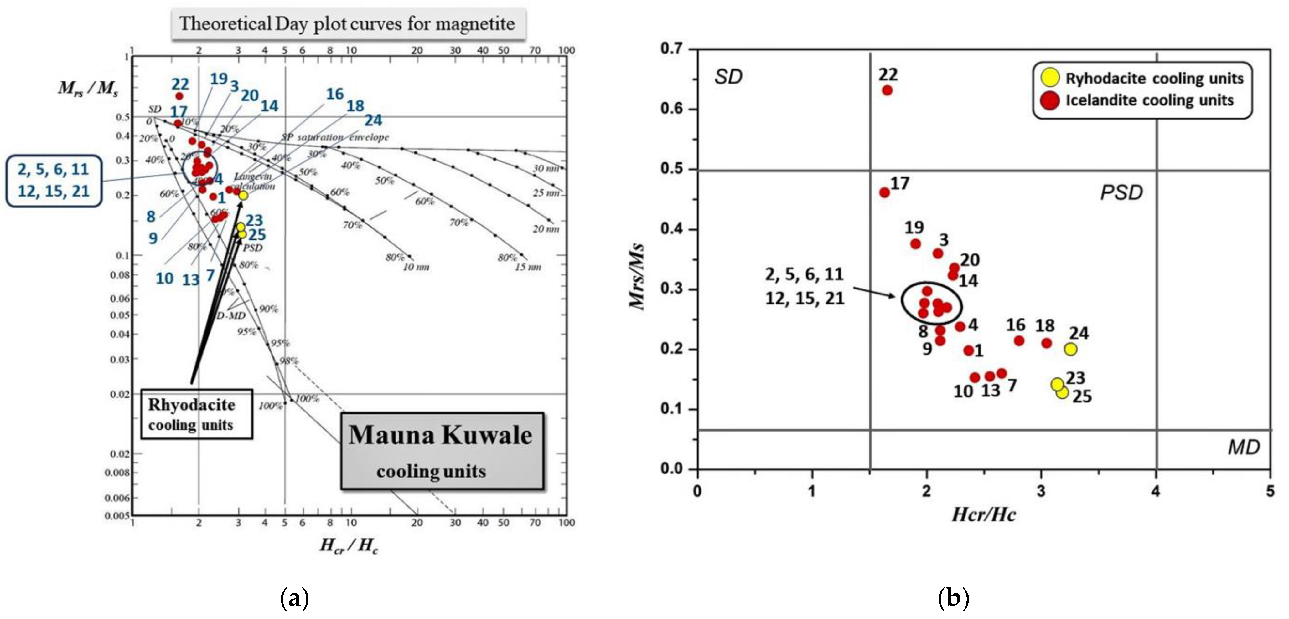
The relative grain size distribution of a mixture can be estimated based on the ratio of hysteresis parameters. The obtained ratio of the saturation remanent magnetization to saturation magnetization Mrs/Ms and the coercivity of remanence to coercivity Hcr/Hc are represented in a Day-Dunlop diagram with binary mixing lines of [
34], in
Figure 6 and
Table 2. It shows that overall, the samples fall in the PSD region but showing properties close to the SD-PSD suggesting a fine granulometry. Exceptionally samples from cooling units 3, 14, 19 and 20, seems to present a coarse granulometry. Only two specimens from cooling units 17 and 22 show a dominant SD magnetic behavior. They also show low MS and magnetic fabric with poorly statistical defined mean directions, which may suggest the combined effect of normal, inverse, or intermediate magnetic fabrics due to single domain particles. For instance inverse magnetic fabric only occurs in single-domain magnetic behavior, i.e., Stoner-Wohlfarth particle assemblages [
35], where the initial susceptibility is minimal (i.e., zero) for particles with magnetic moments along the applied field and maximal in an orthogonal direction. A group of specimens from cooling units 7, 8, 9, 10 and 13, with low values of the Mrs/Ms parameter, approaches the SD-MD mixture region.
The rhyodacite cooling units (23, 24 and 25) are well distinguished from the remaining icelandite cooling units concerning the high field parameters. Indeed, rhyodacite cooling units show the lowest Mrs/Ms values and the highest values of Hcr/Hc, comparing to the typical observed magnetic parameters of the icelandite samples.
7. Discussion and Conclusions
Recently, there has been only one rock magnetic, and anisotropy of magnetic susceptibility (AMS) study of dikes emplaced in the Wai’anae volcano in Oahu Island [
5]. Petrofabric studies of pahoehoe, dikes and silicic rocks lavas have been conducted successfully in regards to the determination of the directions of flows, e.g., [
36,
37,
38]. The present study of lava flows erupted in another location of the same volcano, known as Mauna Kuwale (see
Figure 1) and believed to constitute the roots of the ancient Wai’anae volcano [
39,
40], is the only investigation related to the magnetic mineralogy properties, bulk magnetic susceptibility as well as petrofabrics analyses of these 25 cooling units. It is known that late shield-stage silicic (icelandite and rhyodacite) lavas and dikes are exposed within the caldera region of Wai‘anae Volcano, O’ahu, and comprise the most continuous silicic, sub-alkaline and transitional suites in Hawai‘i. The magmatic evolution during the shield state of the Wai’anae volcano indicates that thus far there is a lack of any tectonic processes to suggest any evidence of rotations, pervasive faulting affecting the Mauna Kuwale which is part of the Wai’anae range [
26].
An interesting issue is that these flows are characterized by a totally different lithology with respect to the rest of the volcanic edifices of the Wai’anae range which are mainly basaltic lavas, while the Mauna Kuwale flows are composed of Icelandites (22 units) and Rhyodacites (3 units).
The overall results of the rock magnetic studies and the AMS experiments can be summarized as follows:
The continuous and partial thermomagnetic cycles of low susceptibility versus temperature k-T experiments, provided three types of thermo-magnetic behavior, termed A, B and C.
Type A is characterized by two components such as titanomagnetites as well as a Ti-rich magnetite phases. Type B is characterized by Ti-poor titanomagnetite as well as a predominance of magnetite that defines the main magnetic carrier. The cooling path show that some amount of higher magnetic mineral was produced by the heating phase as the final magnetic susceptibility is usually higher than the initial magnetic susceptibility. Type C show k-T curves of roughly one single phase of titanomagnetite and Ti-poor magnetite as well. Heating and cooling curves are mostly reversible, demonstrating the predominance of a main magnetic phase of magnetite. One sample displayed a hump with a large range of temperatures from 150–400 °C strongly suggesting the presence of maghemite.
Isothermal Remanent Magnetization (IRM) up to 1.1 T was applied to eight samples showing that 95% of saturation of remanence (SIRM) was obtained at about 0.3 to 0.4 T. The coercivity of remanence, determined by back-field magnetization is always below 60 mT, which indicates the predominance of a magnetic components of low coercivity such as magnetite.
The unmixing of the coercivities performed in the IRM curves acquisitions show characteristically two coercivity components.
A soft phase commonly predominant in percentage, with low B(1/2) < 60 mT, represent usually more than 75%. This component is also characterized by the greatest values of magnetization with SIRM values higher than 300 A/m. A second phase with higher values of coercivity, usually in the interval 160 mT < B(1/2) < 500 mT, minority, representing usually <15% of total coercivity.
The Dispersion Parameter (DP) shows very steady values between 0.25 and 0.30, for the specimens and their corresponding magnetic phases of this study. Exceptionally one sample (MK45b cooling unit 6) shows DP approaching 0.35 for the high coercivity phase, suggesting some non-homogeneity in terms of grain size and composition of the magnetic grain population.
The analysis of a rhyodacite sample (MK188p, flow 25) shows that, despite 95% of SIRM is attained up to 0.2 T, there is evidence of minor but continuous acquisition of magnetization between 0.5 up to 1.1 T. This sample also shows a secondary (≈8%) low coercivity component with B1/2 ≈ 16 mT.
Magnetic granulometry determinations were performed on twenty-seven specimens on the entire set of flow units. The results were represented on the theoretical Day-Dunlop plot curves for magnetite [
34]. The ratios of the remanent magnetization to saturation magnetization Mr/Mrs versus the coercivity of remanence to coercivity Hcr/Hc shows that most of the samples falls in the Pseudo Single-Domain (PSD) region but displaying properties close to the Single-Domain region (SD) suggesting the effect fine granulometry magnetic grains. Exceptionally, samples from flows 3, 14, 19 and 20, seems to present a coarse granulometry.
Samples from cooling units 17 and especially 22 show a predominant SD magnetic behavior. A group of specimens from flows 7, 8, 9, 10 and 13, with low values of the Mrs/Ms parameter, approaches the SD-MD mixture region. The top rhyodacite cooling unit (i.e., 23, 24 and 25) are well differentiated from the remaining icelandite cooling unit as they show the lowest Mrs/Ms values and the highest values of Hcr/Hc, comparing to the typical observed magnetic parameters of the icelandite samples.
Low field magnetic susceptibility (MS) was measured in several samples on each one of the 25 cooling units. Units 17 and 22 show low MS and magnetic fabric with poorly statistical defined mean directions suggesting the combined effect of normal and inverse, or intermediate magnetic fabrics due to single domain particles (
Figure 2). This thought agrees, with the inferred from the magnetic granulometry determinations for these samples, previously referred.
Anisotropy of magnetic susceptibility (AMS) that characterizes the magnetic fabric is used as a tool in rock fabric analyses to investigate the preferred orientation of magnetic minerals in rocks e.g., [
5]. Magnetic anisotropy is low on all measured flows from 1 to 17, with a mean P’ = 1.010, but becomes systematically distinct and high in the rhyodacite flows with a mean P’ = 1.074. Cooling units 2, 6, 11 and 13 shows a magnetic fabric with k
3 axes vertical to sub-vertical which may be denoted as normal for the horizontal to sub horizontal flows. Only cooling units 2 and 15 show high scattered axes. Flow 6 reveal a clear oblate shape with overlapping confidence areas along the magnetic foliation plane while flows 11 and 13 show a triaxial shape of ellipsoid, with k
1 axes roughly horizontal but pointing in different directions ranging from NE to NW. Remaining cooling units show different magnetic fabric with k
3 axes horizontal in flow 10 and sub-horizontal in flow 15.
On cooling units 17 (icelandite), and cooling units 23, 24 and 25 (rhyodacite), despite important variations in anisotropy and shape of ellipsoid (from oblate on flow 23, to prolate on flow 24 and triaxial on flow 25) the magnetic axes show a steady orientation. The k3 axes with a constant orientation, SW to SSW oblique, dipping around 45° and the magnetic lineation axes a very steady azimuth NW nearly horizontal to sub horizontal.
In view of the magnetic mineralogy (predominantly Ti-magnetites and magnetite magnetic mineral phases) and magnetic fabric from the AMS data, we conclude that magnetic fabric is primary, confirming the magmatic origin of the Mauna Kuwale mountain, indicating that both, the icelandite and rhyodacite flows and their corresponding cooling units have not been affected by tectonic deformation.


