Near-Surface 2D Imaging via FWI of DAS Data: An Examination on the Impacts of FWI Starting Model

Abstract

Full waveform inversion (FWI) and distributed acoustic sensing (DAS) are powerful tools with potential to improve how seismic site characterization is performed. FWI is able to provide true 2D or 3D images of the subsurface by inverting stress wave recordings collected over a wide variety of scales. DAS can be used to efficiently collect high-resolution stress wave recordings from long and complex fiber optic arrays and is well-suited for large-scale site characterization projects. Due to the relative novelty of combining FWI and DAS, there is presently little published literature regarding the application of FWI to DAS data for near-surface (depths <30 m) site characterization. We perform 2D FWI on DAS data collected at a well-characterized site using four different, site-specific 1D and 2D starting models. We discuss the unique benefits and challenges associated with inverting DAS data compared to traditional geophone data. We examine the impacts of using the various starting models on the final 2D subsurface images. We demonstrate that while the inversions performed using all four starting models are able to fit the major features of the DAS waveforms with similar misfit values, the final subsurface images can be quite different from one another at depths greater than about 10 m. As such, the best representation(s) of the subsurface are evaluated based on: (1) their agreement with borehole lithology logs that were not used in the development of the starting models, and (2) consistency at shallow depths between the final inverted images derived from multiple starting models. Our results demonstrate that FWI applied to DAS data has significant potential as a tool for near-surface site characterization while also emphasizing the significant impact that starting model selection can have on FWI results.

1. Introduction

Seismic site characterization of near-surface (depths <30 m) conditions is a critical part of rigorous evaluations that needs to be performed for the design of important infrastructure in earthquake-prone areas. The term “seismic” refers to the use of seismic waves (i.e., stress waves) to probe/characterize the stiffness and layering of the subsurface. While seismic site characterization can be performed using invasive methods such as downhole testing, vertical seismic profiling, or seismic cone penetration testing, these methods are expensive and only cover a limited lateral extent. For these reasons, non-invasive methods such as seismic refraction, surface wave testing, or full waveform inversion (FWI) are often preferred as economical alternatives that can be used to rapidly investigate large areas. For near-surface applications, these non-invasive methods are based on making recordings of active-source wavefields using arrays of surface-based receivers. While geophones have been the receiver of choice for many decades, distributed acoustic sensing (DAS) technology is now being investigated as a powerful new sensing tool. DAS uses a fiber optic cable to detect and record stress wave propagation over large distances at high spatial resolution. Combining the unique sensing capabilities of DAS with the powerful imaging abilities of FWI is a logical progression toward improving non-invasive, near-surface seismic site characterization.

FWI is an advanced subsurface imaging technique that inverts the subsurface conditions beneath a site through the iterative fitting of observed (experimental) waveforms collected with arrays of receivers (typically geophones). However, unlike other techniques that only use limited aspects of the observed waveforms, such as wave arrival times for seismic refraction or phase velocity dispersion data for surface wave testing, FWI seeks to invert the entirety of the recorded waveforms through the use of numerical wavefield simulations [1]. This is accomplished by numerically solving a wave equation for candidate subsurface models and comparing the resulting simulated waveforms to those recorded in the field. FWI is also able to provide true 2D or 3D images of the subsurface conditions, as the full lateral extent of the investigated area is inverted simultaneously. This contrasts with alternative methods such as 2D MASW (multi-channel analysis of surface waves), which can only produce pseudo-2D images of the subsurface by combining the results from multiple inherently 1D analyses to form an interpolated 2D image [2,3,4,5].

DAS is a cutting-edge sensing technology that has shown promise in recording stress waves for a variety of geophysical and engineering applications [6,7,8,9,10]. DAS is able to collect data over large scales (e.g., kilometers) while still maintaining high spatial resolution (e.g., 1 m spacing), a feat that is not practically possible with traditional geophone arrays [11,12]. This ability to rapidly collect waveforms at high spatial resolution over very large areas makes DAS particularly well suited for FWI applications. Unfortunately, as DAS is a relatively new technology for recording seismic data, there are very few published studies on FWI applied to DAS data.

This study aims to evaluate the efficacy of applying FWI to DAS data for 2D near-surface site characterization, while also investigating the effect of using various starting models on the FWI results. We first provide important background information on both FWI and DAS. We then present results obtained from performing 2D FWI on DAS data collected at a well-characterized site using four different, site-specific 1D and 2D starting models and discuss the unique benefits and challenges associated with inverting DAS data compared to traditional geophone data. We also examine the impacts of using the various starting models on the final 2D subsurface images and evaluated them based on: (1) their agreement with borehole lithology logs that were not used in the development of the starting models and (2) consistency between the final inverted images derived from multiple starting models. Our results demonstrate that FWI applied to DAS data has significant potential as a powerful tool for near-surface site characterization while also emphasizing the significant impact that starting model selection can have on the results.

2. Background and Prior Near-Surface Applications of FWI

FWI has existed since the 1980s, when Lailly [13] and Tarantola [14] proposed the minimization of the misfit between observed and simulated waveforms in the time domain through a least-squares optimization procedure. It has been the subject of increasing interest for site characterization since Pratt [15] introduced and demonstrated a procedure that allows for relatively fast local optimization inversions [16,17] and has been adopted for a wide variety of geophysical applications [1]. While inverting for material parameters such as shear wave velocity (V_S) and compression wave velocity (V_P) are of particular interest to engineers, FWI is also capable of evaluating any other material parameters that influence seismic wave propagation, including density (ρ) and attenuation [18]. While FWI has been used across a wide variety of spatial scales, herein we will focus primarily on how FWI can be applied to observe active-source seismic waveforms for near-surface characterization (depths <30 m).

By using the entire seismic record and accurately modeling the waveform physics in an iteratively refined digital twin, FWI can investigate the subsurface conditions more rigorously and better match the distribution of energy in the observed waveforms than other techniques that only use limited aspects of the waveforms [18]. However, unlike inversions of surface wave dispersion data, which often use global search optimization methods to account for inversion non-linearity and non-uniqueness, FWI is almost always performed using local search optimization methods [1,16,17], as the already computationally expensive numerical methods used to model wave propagation make the use of intensive global search methods highly impractical. While local search methods are much less computationally intensive, they are more susceptible to becoming trapped in local minima and, as such, are more significantly influenced by the inversion starting model [19]. This has been demonstrated for both traditional surface wave dispersion [20] and full waveform inversions [21,22].

Applying FWI in the near surface can be particularly challenging because materials can change rapidly over short distances (vertically and laterally), from very soft unconsolidated sediments to stiff rock, and the various components of the elastic wavefield (i.e., compression, shear, and surface waves) are mixed together, having not yet propagated far enough to spread out from one another [23,24]. Due to these challenges, FWI has primarily been limited to larger-scale applications, characterizing depths where body waves dominate the wavefield [16]. However, a number of researchers have explored applications of FWI in the near surface.

Gélis et al. [25] utilized a synthetic 2D example to investigate the joint FWI of body and surface waves in the frequency domain. They utilized a simple model with localized anomalies present within a known background medium and found that simultaneous inversion of body and surface waves yielded poor results due to surface waves dominating the wavefield, but inversion of first body waves and subsequently surface waves was able to successfully reconstruct the anomalies within 2D V_P and V_S images. Romdhane et al. [26] performed a synthetic study to examine the applicability of frequency–domain FWI to analyze Rayleigh waves in 2D. They developed a synthetic data set using a 2D model with complex topography and subsurface conditions based on a landslide site. They found that, similar to Gélis et al. [25], surface waves dominated the recorded wavefields, preventing the consideration of high-frequency body waves and creating challenges in sequential inversion of individual frequencies. However, when they performed simultaneous inversion of groups of damped frequencies to allow for the gradual introduction of surface wave content, the shallow structure with the 2D model could be successfully identified.

Tran and McVay [27] demonstrated the use of time-domain 2D FWI on field data collected using an array of 24, 4.5-Hz geophones with 1.5 m spacing. They utilized a 1D starting model with V_S increasing linearly with depth and a constant value of Poisson’s ratio to develop a final 2D V_S image beneath the array. They successfully identified a high-velocity layer within the resulting 2D V_S image that agreed reasonably well with standard penetration test N-values from a borehole within the array. Similar to Tran and McVay [27], Groos [28] applied 2D FWI to waveforms recorded at a site with low lateral variability using a 1D starting model with a linear V_S gradient and a separate 1D model using the joint inversion of compression wave first-arrival times and Fourier–Bessel expansion coefficients. They found that FWI did not introduce any significant lateral variability into the inverted 2D models, and changes were limited to the top 6 m of the model due to limited low-frequency content of the recorded wavefields. They found that while there were moderate differences in V_S, the waveforms from both models fit the field waveforms almost equally well. Kallivokas et al. [29] applied 2D FWI to field data collected in Austin, Texas. They used a 1D starting model where each parameter was either constant or varied linearly with depth and found that the resulting 2D V_S images compared well with 1D V_S profiles from spectral analysis of surface waves (SASW) testing performed at the site.

The studies noted above have all been limited to the use of simple 1D starting models, consisting of materials with constant or linearly increasing parameters with depth. Groos et al. [30] utilized a slightly more complex 1D starting model, with a V_S profile consisting of a linear gradient over a constant half-space, to produce a 2D subsurface image. They applied the geometric spreading corrections developed by Forbriger et al. [31] and used their resulting 2D model to produce simulated waveforms that fit the recorded waveforms better than those produced with a 1D V_S profile from traditional inversion of Rayleigh wave dispersion data. They attributed these improvements in part to the greater spatial resolution of the final inverted FWI 2D model, as the 1D profile was limited to only two layers over a half-space. Fathi et al. [32] applied 3D FWI to data collected at the Garner Valley NEES@UCSB test site. They utilized a 1D starting model developed by smoothing a 1D V_S profile from SASW testing performed at the site. Fathi et al. [32] targeted a subset of the waveforms recorded at the site in their inversions and used the rest to validate their inversion. Simulated waveforms generated with their final 3D model showed good agreement with the waveforms not used for inversion and demonstrated for the first time that FWI could be successfully used for 3D near-surface characterization of V_S and V_P. Since then, multiple studies have explored the development of FWI starting models based on site-specific data. Köhn et al. [33] used seismic refraction to develop a 2D starting model for the characterization of the Fossa Carolina canal by applying 2D FWI to Love waves, producing a 2D V_S image that agreed well with excavations at the site. Wang et al. [34] performed 3D FWI on data collected at the Yuma Proving Ground in Arizona to detect tunnels at the site. They developed their 1D starting model based on smoothed results from MASW and refraction data collected during previous studies and found that, while the resulting 3D models did not change much relative to the 1D starting models in areas without known anomalies, they were able to successfully identify low-velocity zones corresponding to tunnels.

Despite the increased use of more complex and site-specific starting models, very little work has been conducted on examining the impacts of various starting models on the inversion results. Beller et al. [35] examined the impact of using various starting models based on either wave velocities, impedance values, or elastic moduli on 2D FWI analyses characterizing the lithosphere. They found that a 1D global reference model provided a reliable starting model if layering within the model was sufficiently smoothed so that it could be properly updated by the FWI algorithm. Beller et al. [35] also found that starting models that were too simple, such as linear gradient models, could result in the density parameter of the model being over-updated during the inversion process at the expense of the velocity parameters. However, the scale mismatch between their work, inverting recordings of earthquakes thousands of miles away to characterize the subsurface at the crustal level, and the use of FWI for near-surface characterization are significant, and their findings relative to near-surface applications need to be evaluated. Pan et al. [22] examined the sensitivity of the misfit functions used in FWI and MASW. They used a synthetic two-layer model and evaluated the contours of the misfit function as a function of the V_S values of those two layers. Pan et al. [22] found that the FWI misfit contained more local minima than the MASW misfit and that the region leading to the global minima for FWI was narrower than for MASW. Based on that behavior, they found that FWI was more susceptible to local minima convergence than MASW and, therefore, more significantly influenced by the choice of starting model. Pan et al. [22] did not, however, perform any inversions to compare how the results from a poor starting model might compare to those from a better one.

Vantassel et al. [24] utilized two and three-layer synthetic ground models to generate synthetic target waveforms for 2D FWI. They then inverted each of these data sets using four different starting models. The first two for each inversion were 1D starting models with either constant or linearly varying V_S values as a function of depth, similar to those used in many of the studies discussed above. The third starting model for each data set was developed by performing MASW inversions on synthetic waveforms generated with the true V_S model to produce a single, 1D discretized median profile from the results of multiple inversion parameterizations. Finally, the fourth starting model for each inversion was developed using a convolutional neural network (CNN). After inverting the synthetic data sets using each starting model, Vantassel et al. [24] found that, while they could match the target waveforms well using three of the four starting models (the inversions performed with the homogeneous starting models failed to update), the subsurface models changed relatively little during the inversion process. They also found that the CNN-derived 2D starting models were able to produce better fits to the target data prior to FWI than the 1D starting models could produce after FWI was performed, suggesting that CNNs are a promising method for developing 2D FWI starting models.

This study seeks to further investigate the impact of starting models on FWI results by inverting data collected in the field using multiple site-specific starting models based on the results from alternative site characterization techniques.

3. Background and Prior Near-Surface Applications of DAS

DAS’s ability to collect high-resolution data over large scales is accomplished through the use of a fiber optic cable and a laser interrogator unit (IU). The IU generates pulses of laser light that travel down the cable. A portion of the light is reflected back toward the IU in the form of Rayleigh backscatter [36]. The IU measures this backscatter and, using interferometry, is able to measure the change in optical phase between locations where the scattering is sampled [37]. The distance between these locations is known as the gauge length and is controlled by the IU configuration. These phase change (dφ) values can be converted to axial strain (${ϵ}_{DAS}$) along the fiber using the relationship shown in Equation (1) [38].

$${\epsilon }_{DAS}=\frac{\mathsf{\Lambda } \mathrm{d}\mathsf{\phi }}{4\mathsf{\pi }\mathrm{ng}\mathsf{\xi }}$$

(1)

Here, Λ is the average optical wavelength of the laser, n is the group refractive index of the fiber, g is the gauge length, and ξ is the photoelastic scaling factor for longitudinal strain in the fiber.

This measurement of strain through phase change is one of the key differences between DAS and geophones. For geophones, the raw waveforms represent the change in electrical potential (voltage) caused by the wire-wrapped mass inside the geophone oscillating within a magnetic field. Similar to how the raw phase change measurements of DAS can be converted to strain, these voltages are proportional to the velocity of the geophone housing for frequencies above the geophone’s natural frequency. Note that for frequencies near and below the geophone’s natural frequency, the relationship is deterministic but non-linear. Assuming good coupling with the ground surface, these scaled measurements can be taken as the particle velocity of the seismic waves in the soil. This change from measuring particle velocity with geophones to measuring axial strain with DAS requires particular attention when performing FWI on DAS data and will be discussed in greater detail below. Importantly, while geophone records represent discrete measurements of particle velocity at set locations, DAS records are instead distributed measurements of strain over the gauge length. Effectively, the cable acts as a linear array of distributed strain sensors with the spacing between channels set by the IU. Channels along the entire length of the cable are recorded simultaneously, yielding the ability to collect data more efficiently than with traditional geophone arrays, which are often limited to a specific number of channels based on the equipment available.

The efficacy of using DAS to collect surface wave records for MASW has been examined in several studies [9,39,40,41,42], which utilized DAS for active-source MASW surveys and compared the results to co-located arrays of traditional sensors. Galan-Comas [39] performed a rigorous MASW survey using side-by-side geophone and DAS arrays that were 70 m long with shots at multiple locations off each end of the arrays. The dispersion data extracted from both arrays had excellent agreement within the shared frequency band, with the only significant difference being that the DAS array only resolved dispersion data up to 23 Hz, while the geophone array resolved data up to 56 Hz. Lancelle et al. [42] collected data from a DAS array with geophone and accelerometer data also collected along various portions of the fiber optic cable. Lancelle et al. (2021) extracted dispersion data from all three receiver types using a modified MASW procedure, finding excellent agreement at high frequencies but some variation at lower frequencies. Lancelle et al. [42] also inverted the dispersion data from the DAS and accelerometer arrays, finding that the resulting 1D velocity profiles agreed well with each other and a borehole log from the site.

Vantassel et al. [9] extracted multi-modal Rayleigh-wave dispersion data from DAS data recorded using two co-located fiber optic cables and from a traditional geophone array on the same alignment, finding excellent agreement between all three surface wave modes from both the DAS and geophone records. Vantassel et al. [9] further demonstrated that special considerations for channel spacing and gauge length need to be made when processing DAS data for MASW; the minimum wavelength resolved must be greater than either two-times the channel spacing, which is analogous to the Nyquist–Shannon sampling theorem in space, or the gauge length, which causes attenuation and phase corruption at short wavelengths. FWI has an advantage over MASW in that the gauge length effect is accounted for implicitly in the forward problem simulation.

As mentioned above, there is relatively little literature concerning the combination of FWI and DAS. Most of the publications discussing the application of FWI to DAS data are concerned primarily with data collected in wellbores for reservoir characterization and monitoring, a selection of which are discussed here. Egorov et al. [43] demonstrated the application of FWI on DAS data for vertical seismic profiling in a wellbore. They collected DAS data down to a depth of 1600 m with a 1 m channel spacing and 10 m gauge length. In order to apply standard FWI procedures intended for geophone data, Egorov et al. [43] developed and applied a regularized approach to convert the DAS data to particle velocity while compensating for gauge length and pulse width. After inverting the converted data, they found that the resulting V_P profile agreed with well log results, having a correlation coefficient of 0.85. Eaid et al. [44] performed simultaneous FWI of synthetic DAS and geophone waveforms from a horizontal well in both simple and complex models. They found that the combination of DAS and geophone data complimented one another for wellbore applications and provided more accurate estimates of the subsurface parameters than individual inversions. Eaid et al. [45] applied the same methodology they used previously on synthetic data to the joint inversion of DAS and accelerometer data collected in the field at a test well. They again found that the two data sets complemented each other, producing inversion results that agreed well with the observed data.

Applications of FWI to DAS data collected at or near the surface are less well documented but have been explored by some researchers. Liu and Li [46] utilized a synthetic model to examine the differences in FWI results from simulated DAS and geophone data sets. They found that the dispersion data from synthetic DAS and geophone waveforms agreed well, with some deviation at low frequencies. Liu and Li [46] inverted the DAS data both directly and by converting them to particle velocity. Converting the DAS data to particle velocity before inversion significantly reduced the quality of the results, while direct inversion of the DAS data produced results that agreed well with both the true model and FWI results from synthetic geophone data. Liu et al. [47] applied the methodology of Liu and Li [46] to DAS data. The data were collected from a 184 m linear array with a 1 m channel spacing and 10 m gauge length. A total of 23 shots were recorded along the line with a spacing of 8 m. The data were inverted in three stages with frequency bands of 0 to 10, 0 to 15, and 0 to 20 Hz. Liu et al. [47] found that the resulting 2D V_S image agreed well with a pseudo-2D V_S image from 2D MASW testing at the site.

The most comprehensive examination of FWI applied to DAS data collected near the surface is provided by Pan et al. [48]. They performed FWI on DAS data collected from a trenched 533 m long cable with a 10 m gauge length and an unspecified, but likely 10 m, channel spacing. They used a 1D starting model with V_P values following a linear gradient in the top 60 m before transitioning to V_P values obtained from well log measurements below that depth. The V_S values for the staring model were based on surface wave inversion results in the top 100 m before transitioning to V_S values obtained from well log measurements. Both the V_P and V_S profiles were smoothed with a Gaussian filter. Pan et al.’s [48] FWI model was 200 m deep and 533 m wide. They were able to successfully invert the DAS data obtained from seven shot locations near one end of the DAS array. Pan et al. [48] converted the DAS data to displacement prior to inverting it, and while they produced a model that fit the observed data well, very little change was observed in the inverted 2D V_S image above a depth of 30 m, as the study was primarily concerned with characterizing deeper features. Given the limited amount of literature about the application of FWI to DAS data for near-surface characterization, particularly without conversion of the data to displacement or velocity, we feel that the present study will offer a beneficial demonstration of the application of FWI to DAS strain data for characterization of the top 30 m of the subsurface, an area of significant interest to geotechnical engineers. However, before discussing the specifics of the field testing performed in this study, it is important to have a good understanding of how FWI is performed, particularly with regard to factors that will influence its application to DAS data.

4. FWI Workflow for DAS Data

The general workflow of FWI follows the same basic steps as all seismic inversion techniques. These steps can be stated generally as follows: (1) processing the observed waveforms and selecting which ones will be targeted in the inversion, (2) developing a candidate starting ground model to represent the subsurface, (3) simulating an analog to the target data based on numerical wave propagation through the candidate starting model, (4) determining the level of agreement (misfit) between the simulated and targeted data, and (5) developing a model update that reduces the misfit. Steps 3 through 5 are repeated iteratively to optimize the ground model until the lowest possible misfit is obtained. When inverting DAS data, special attention is required when performing steps 4 and 5.

The first step of FWI, processing and selecting the observed waveforms to produce inversion targets, is also the most straightforward one. All FWI analyses start out with some set of observed data, often wavefield recordings from geophones, or in the case of this study and as is likely to become more common in the near future, DAS. As discussed above, the measurements provided by geophones and DAS directly relate to the particle velocity and axial strain, respectively, of the soil. No matter the acquisition method used, it is important that the observed data be directly relatable to a physical parameter that describes the motion or state of the soil, such as displacement, velocity, or strain, which can be simulated. Regardless of which parameter the observed waveforms represent, they must be processed before they can be used for inversion.

There are several processing steps that are often applied to the observed data, including correlation, source correction, and filtering. The observed waveforms used for FWI are often cross-correlated with a recording of the source output for each shot location. This is generally performed when a vibratory source is used to simplify the analysis by producing observed data that mimic the result of a short-duration impulse source. While this type of cross-correlation is used in many tomography methods, it is especially important for FWI to reduce the duration of the wavefield simulations that need to be performed during the inversion process. When this cross-correlation is performed, a delta function, the idealized autocorrelation of the recorded source output, is frequently used as the source in the wavefield simulations. For any FWI performed in 2D, a source-type correction must also be applied to the observed waveforms [31,49]. This is because the observed waveforms were originally collected in a 3D environment (i.e., the real world) with a point source (or at least an approximation of one), whereas waveforms simulated in 2D environments are produced by a line source extending infinitely in the third dimension that is not being simulated [31]. As such, the amplitude of the observed waveforms must be adjusted to account for the geometric spreading that occurs in 3D space but not in the 2D simulation. Forbriger et al. [31] proposed several correction algorithms that are applied to the observed data in the frequency domain and are tailored for various conditions, such as shallow seismic waves, including surface waves and reflected body waves. The final part of processing the observed data is to filter them to the frequency band of interest. Then, once the observed data have been fully processed, the individual waveforms that will be used as the targets of the inversion are selected. While it is generally best to provide the inversion with as much information as possible, waveforms recorded from certain shots or receivers may be excluded from the inversion targets for a variety of reasons, including low signal quality or proximity to the source. All these processing steps were applied to the DAS data inverted in this study, including correlation to the recorded source output, source-type correction, band-pass filtering, and selection of certain waveforms. The specific details of the observed DAS waveforms used in this study and how they were processed are discussed in later sections.

Once the target data have been selected, the second step of FWI is to establish an initial candidate model to represent the subsurface conditions. This model needs to cover the entire area or volume of interest. For 2D inversions, such as those performed in this study, the starting model consists of a cross-section of some specified spatial resolution. Each point in the starting model is defined by at least five parameters: V_S, V_P, ρ, and the quality factors, Q_κ and Q_μ, assuming that wavefield simulations will occur in an elastic medium with attenuation. The first three parameters will likely be familiar to most engineers, geophysicists, and seismologists, while the quality factors Q_κ and Q_μ may not. They characterize the attenuation of compression and shear waves, respectively, within the model [50]. Some models may have additional parameters to define things such as anisotropy of the materials in the model. The values for these parameters can be set in a wide variety of ways, including basing them off the results of previously performed testing or assuming reasonable generic values based on other information known about the site. As discussed above, the local search optimization approaches typically used for FWI can be significantly impacted by the starting model. Therefore, it should be as close as possible to the true subsurface conditions of the site. This study used four different starting models with parameters based off high-quality site characterization results from multiple methods, which are discussed in greater detail below.

The third step of the FWI process is to simulate a counterpart to the target waveforms. This requires a full-wave simulation to be performed using the candidate starting model [1,17] by efficiently solving the viscoelastic wave equation. For extremely simple models, the wave equation has a closed-form solution, but for any model complex enough to be of interest, a numerical solution is required [50]. The most common type of approach to modeling seismic wavefields is finite difference methods, due to their balance of accuracy and efficiency [51]. Various finite difference methods for simulating of seismic wave propagation have been developed to handle models with increasing complexity [52,53,54,55], with some implemented in FWI programs such as Devito [56] and DENISE [53,57,58]. However, finite difference methods are limited when applied to models with complex topology or subsurface conditions [50]. Finite-element approaches offer alternative numerical solutions that do not suffer from these limitations but are less computationally efficient [59]. To address this, analysts have turned to the spectral element method [50,60,61,62], a variant of the finite element method. The Salvus software suite [50] utilizes a refined implementation of the spectral element method and was used to perform all steps of the inversions in this study, from processing of the observed data to optimization of the ground models. Specifically, Salvus utilizes the time-domain isotropic elastic wave equation with linear viscoelastic rheology. A full derivation of the relevant equations can be found in Fitchner [63] or van Driel and Nissen-Meyer [64]. No matter which method is used, the end results of these forward simulations are simulated waveforms matching the parameter (strain, velocity, etc.) of the observed waveforms recorded by receivers placed within the model.

The fourth step of the inversion is to compare the simulated and observed waveforms and to calculate a misfit value representing their level of agreement. The most common form of this misfit is simply the L2 norm of the residuals. However, as will be discussed in more detail below, FWI is almost always performed using local search optimization and is vulnerable to becoming trapped in local minima, especially when an L2 misfit is utilized [21,65,66,67]. The primary cause of local minima when utilizing an L2 misfit is cycle skipping, where the simulated and observed waveforms are out of phase with one another by more than half a wavelength. As a result, an L2 misfit can cause the optimization algorithms to attempt to shift the waveforms completely out of phase to achieve a lower misfit value, trapping the inversion in local minima. Additionally, if the shape of the waveforms or individual arrivals are different, a misfit based on cross-correlation [68] would be of little help. These challenges are particularly relevant to near surface applications of FWI, as the surface waves that dominate the near surface wavefield are complex and lack distinct arrival times. Additionally, approximation of the source, conversion from 3D to 2D space, and imperfect coupling between the source, ground, and receivers can all create even more complexity. This means that even sophisticated starting models are likely to produce initial simulated waveforms that are fairly different than those recorded in the field. To mitigate these problems, different misfit functions have been proposed, including implementations of deconvolution [69], envelope-difference [70], and optimal transport [18,71]. The inversions performed in this study used the graph space optimal transport distance (GSOTD) misfit algorithm developed by Métivier et al. [71] and implemented in Salvus, as shown by Equations (8)–(10) in Boehm et al. [72], wherein the simulated and observed waveforms are first converted to discrete point clouds before being globally compared in graph space using optimal transport distance techniques. This misfit is designed to try to match the overall structure of the observed waveforms to mitigate cycle skipping and allow for energy to be redistributed as needed. The use of optimal transport misfits for FWI is an ongoing and promising area of study (Provenzano et al. [73], da Silva et al. [74]). When computing the misfits in this study, both the simulated and observed waveforms were normalized by their respective L2 norms. This was performed to account for two things: the significant uncertainty concerning the exact amount of force that was imparted into the ground by the vibroseis source and later transferred through friction to the DAS cable, and any scaling introduced into the observed waveforms during the cross-correlation process. Computing the misfit is also the first step where the inversion of DAS data diverges from standard FWI of geophone data. These differences, and how Salvus addresses them, are discussed below.

Once the misfit for the candidate starting model has been calculated, the fifth and final step is to modify and optimize the original model to produce a lower misfit model. To do this, the gradients of the model parameters must first be calculated. In FWI, this is done through the use of adjoint simulations [1,75]. The source functions used in these simulations, known as adjoint sources, represent the discrepancies between the simulated and observed waveforms for each receiver, as defined by the selected misfit function. For example, the adjoint sources for a standard L2 misfit are simply the residuals between the two waveforms, but adjoint sources for alternative misfit functions, such as the GSOTD misfit used in this study, can be more complex to develop. Additionally, the derivation of the adjoint sources requires some care when inverting DAS strain data rather than particle velocity or displacement data. This is due to the fact that, while those variables are point measurements, strain is, by its very nature, a distributed measurement representing the deformation of a material over some extent. Furthermore, strain is not a primary state variable of the wave equation. Salvus implements a novel approach to this challenge to allow for the direct inversion of strain data without needing to convert it to velocity or displacement, as in some of the prior studies discussed above.

In order to explain how Salvus addresses this issue, it is important to understand in greater detail how adjoint sources are developed. To perform adjoint simulations, Salvus utilizes the spectral element method and the viscoelastic wave equation formulated with the displacement field (u) as the primary state variable [50]. This means that the adjoint sources used in the inversion also need to be derived in terms of u. If the observed data correspond to displacement, this is relatively simple. For example, the misfit function, χ(u), for an L2 misfit would be defined according to Equation (2):

$$\chi \left(\mathrm{u}\right)=\frac{1}{2} \parallel \mathrm{u}-{\mathrm{u}}_{\mathrm{obs}}{\parallel }^2,$$

(2)

where u is the simulated displacement, and u_obs is the observed displacement and would result in adjoint sources that are simply the residual: u_obs − u. However, it is often necessary to compute misfit and adjoint sources for other fields, such as particle velocity when inverting geophone data or, in the case of this study, strain when inverting DAS data. For velocity, this can be conducted by simply invoking the chain rule and time derivative of the displacement field. The elastic wave equation can also be formulated with velocity as the primary state variable instead of displacement, but this precludes the inclusion of attenuation within the simulation. For strain, this process is more complex, as it is a spatial derivative of displacement rather than a time derivative such as velocity. Thus, deriving the misfit function and adjoint sources for strain requires the use of a derived quantity, q, which is defined by Equation (3):

$$\mathrm{q}=\mathrm{q}\left(\mathrm{u}\right)=\mathit{Ɗ}\mathrm{u},$$

(3)

where Ɗ is a linear operator applying a spatial derivative to the displacement field, u. Returning to the example of an L2 misfit, this results in χ(u) defined according to Equation (4):

$$\chi \left(\mathrm{u}\right)=\frac{1}{2} \parallel \mathrm{q}\left(\mathrm{u}\right)-{\mathrm{d}}_{\mathrm{obs}}{\parallel }^2,$$

(4)

with q(u) as the derived strain field based on the simulated displacements, and d_obs is the observed strain data. Similar substitutions can be made when using more complex misfit formulations, such as the GSOTD approach used in this study [71], but the equations are more complex, and an in-depth examination of the misfit formulation is outside the scope of this paper.

In order to derive the adjoint sources, we need the partial derivative of the misfit function, χ, with respect to the displacement field, u. This partial derivative can be defined generally for any form of χ according to the first part of Equation (5):

$$\left(\frac{\partial }{\partial \mathrm{u}}\chi ,\mathsf{\delta }\mathrm{u}\right)=\left(\frac{\partial }{\partial \mathrm{q}}\chi ,\frac{\partial }{\partial \mathrm{u}}\mathrm{q}\left(\mathrm{u}\right)\mathsf{\delta }\mathrm{u}\right)=\left(\frac{\partial }{\partial \mathrm{q}}\chi ,\mathit{Ɗ}\left(\mathsf{\delta }\mathrm{u}\right)\right),$$

(5)

where it is written as a directional derivative representing how the misfit function changes when a perturbation, with direction δu, is applied to the simulated displacement field. However, because the comparison that occurs within the misfit function is to the derived field q, and not u, the chain rule is used to obtain the derivative with respect to q, as shown by the second part of Equation (5). While this application of the chain rule introduces additional terms to the right side of the directional derivative in the form of the partial derivative of q with respect to u, they can be simplified as the application of the linear operator Ɗ to the perturbation δu. Again, returning to the L2 misfit as an example, the left side of the derivative would be the residuals of q and d_obs, as shown in Equation (6):

$$\left(\left(\mathrm{q}\left(\mathrm{u}\right)-{\mathrm{d}}_{\mathrm{obs}}\right),\mathit{Ɗ}\left(\mathsf{\delta }\mathrm{u}\right)\right),$$

(6)

However, for the formal definition of the adjoint source as a vector source, we would need to isolate δu on the right-hand side of the derivative. This can be done by taking the adjoint, Ɗ^†, of the linear operator Ɗ and applying it to the derivative according to Equation (7):

$$\left({\mathit{Ɗ}}^{†}\left(\mathrm{q}\left(\mathrm{u}\right)-{\mathrm{d}}_{\mathrm{obs}}\right),\mathsf{\delta }\mathrm{u}\right),$$

(7)

While this is simple in theory, determining the adjoint Ɗ^† is nontrivial when Ɗ includes spatial derivatives, as is the case here. To address this challenge, we can take advantage of the weak form of the elastic wave equation, which is one of the key aspects of the spectral element method. When working with the weak form of the wave equation, moment tensor sources are defined according to Equation (8):

$$\left(\mathrm{M},\mathsf{\epsilon }\left(\mathrm{v}\right)\right),$$

(8)

where M is a moment tensor with six components in 3D or three components in 2D, ε is the strain tensor as a function of some displacement, and v is a vector test function. This form matches that of Equations (5) and (6) with the same number of components on both sides of the derivative, and as such, adjoint sources for strain inversions can be applied as moment tensor sources rather than vector sources, eliminating the need to calculate the adjoint Ɗ^†.

This approach, however, assumes that we have observed data corresponding to all components of the strain tensor. This is not the case for DAS, where only a single component, the axial strain in the direction the cable is running, is measured. This mismatch can be rectified by adding additional elements to the linear operator Ɗ, so that rather than simply providing ε(u), it is now defined according to Equation (9):

$$\mathit{Ɗ}\mathrm{u}=e^T\mathsf{\epsilon }\left(\mathrm{u}\right)e,$$

(9)

where e is a direction vector representing the direction of the DAS cable in 2D space, and e^T is its transpose. For the L2 misfit example, this results in adjoint sources with the form shown in Equation (10):

$$\left(\frac{\partial }{\partial \mathrm{q}}\chi ,\mathit{Ɗ}\left(\mathsf{\delta }\mathrm{u}\right)\right)=\left(\left(\mathrm{q}\left(\mathrm{u}\right)-{\mathrm{d}}_{\mathrm{obs}}\right),e^T\mathsf{\epsilon }\left(\mathsf{\delta }\mathrm{u}\right)e\right)=\left(\left(\mathrm{q}\left(\mathrm{u}\right)-{\mathrm{d}}_{\mathrm{obs}}\right)e{e}^T,\mathsf{\epsilon }\left(\mathsf{\delta }\mathrm{u}\right)\right),$$

(10)

where the strain caused by the perturbation δu has been isolated on the right site of the derivative. In this case, the adjoint source consists of the three unique components of ee^T, as it is symmetrical, scaled by the scalar residual values of q(u)-d_obs. Finally, moment tensor adjoint sources can be defined generally for misfit functions of all forms using Equation (11):

$$\left(\left(\frac{\partial }{\partial \mathrm{q}}\chi \right)e{e}^T,\mathsf{\epsilon }\left(\mathsf{\delta }\mathrm{u}\right)\right),$$

(11)

and by simply taking the partial derivative of χ with respect to q, which is the same as taking the partial derivative with respect to u for inversions where the observed data represent displacement. This process was used to generate adjoint sources for the GSOTD misfit function used in this study.

Once the adjoint sources have been developed, they are then simulated in reverse time to generate the adjoint wavefield. The gradients are calculated by cross-correlating the adjoint and forward wavefields for each shot [1,14,76] and integrating in time. This requires simultaneous access to both the forward and adjoint wavefields, which would normally require a very large amount of memory. As the inversions in this study were run on a desktop computer, they utilized checkpointing techniques and wavefield compression implemented in Salvus, trading off memory requirements for additional computations. Once that has been completed, the portions of the model where the correlation is not zero provide the gradients, representing the areas of the model that need to be altered to better fit the observed data [14]. The gradients developed in this study were preconditioned and scaled using a combination of source cutouts (selective muting), model-dependent smoothing using a diffusion filter, and a trust-region-based limited memory Broyden–Fletcher–Goldfarb–Shanno (L-BFGS) algorithm. The source cutouts and model-dependent smoothing were applied to the gradients from individual shots prior to being summed together and are discussed in greater detail in a later section.

The model updates were scaled based on the L-BFGS trust region radius, with the first update limited to 5% deviation. For all subsequent updates, the L-BFGS algorithm [19,77] was used to calculate an approximation of the inverse Hessian vector products, which provided information about the local curvature of the misfit as a function of the inversion parameters, as demonstrated by Boehm et al. [78], and predicted the misfit reduction for the proposed update. Forward simulations were then performed for the updated model, and the true updated GSOTD misfit values were calculated. If the average GSOTD misfit across all shots was reduced, the new model was accepted; if not, it was rejected. This process of proposing and evaluating candidate models was repeated with updates scaled smaller and smaller, until an updated model that successfully reduced the misfit was found. The trust region radius was then updated based on the result, with updated models that reduced the misfit more than initially predicted generally causing the radius to increase, leading to larger changes in proposed updates, and misfit reductions less than predicted causing a decrease, leading to smaller proposed changes. This process of forward modeling to produce simulated waveforms, computation of the misfit, and development of an updated model that reduces the misfit is then repeated iteratively until the final model is believed to be a reasonable representation of the subsurface conditions.

5. DAS Data Acquisition and Processing

The DAS data used in this study were collected at the NHERI@UTexas [79] Hornsby Bend test site in Austin, TX. Additionally, geophone and borehole data collected at the site were used in the development of starting models for the FWI analysis. An overview of the layouts for the testing performed at the site is shown in Figure 1. The fiber optic array was installed at the site by first surveying the endpoints of a 200 m long alignment, which was then trenched to a depth of 10–15 cm. Two fiber optic cables were run parallel to one another in the trench: one from NanZee Sensing Technology and one from AFL. The trench was then backfilled and compacted using a skid-steer loader. The two cables were spliced together at the far end of the array (i.e., 200 m), such that DAS data could be recorded simultaneously on both, with the NanZee cable connected to the IU at the near end of the array (i.e., 0 m), and the AFL cable at the near end terminated appropriately to avoid reflections. However, only the data from the NanZee cable were used in this study, as both Vantassel et al. [9] and Hubbard et al. [80] found that there is no significant variation between the DAS data collected using each cable. The NanZee cable (NZS-DSS-C02) is a single-mode, tightly buffered cable, meaning it contains a single glass fiber with a hard coating. The cable is designed for strain-sensing applications with braided steel reinforcement and a textured polyethylene sleeve to protect the fiber and to help transfer strains to the fiber from the surrounding medium. This cable was selected for this project due to these specific characteristics, as well as the fact that it has been used successfully in several previous engineering projects where good coupling to the ground was important [81]. Furthermore, while not a focus of this study, both Vantassel et al. [9] and Hubbard et al. [80] performed extensive comparisons between DAS data and geophone data collected at the Hornsby Bend site and found them to yield nearly identical frequency/wavelength resolution and waveform amplitude and phase, respectively.

The DAS data for this study were collected using an OptaSense ODH4+ IU owned by NHERI@UTexas. The data were originally collected with a ping rate of 20 kHz to improve the signal-to-noise ratio, which was decimated down to 1 kHz before processing to make sure that file sizes and computational requirements were reasonable. The ODH4+ is a variable gauge length IU, meaning that the gauge length can be adjusted by the user to suit specific project needs. Here, the gauge length was set to 2.04 m, the shortest option. The channel spacing was also set to the minimum value available for the ODH4+, which was 1.02 m. Both of these values were chosen to maximize the wavelength bandwidth that can be properly recorded by the array. As discussed above, the individual DAS channels are not point measurements with set positions, such as with geophone arrays, but are instead distributed measurements with positions dependent upon the exact length of fiber between the IU and each individual channel. The position of each channel can generally be assumed to be the midpoint of each gauge length and can be roughly determined using a tap test. For this array, tap tests were performed starting at the 0 m mark and then every 50 m laterally until 200 m. Each test was performed by tapping on the ground at the known location and then by determining which channel had the highest amplitude response. The results from the tests at 50, 100, and 150 m were used to establish the nearest channels, which were then used, along with the 1.02 m channel spacing, to fix the channel numbers relative to the location of the array. The results from 0 and 200 m were used to determine the extent of usable DAS channels for each end of the array. Overall, 196 channels on the NanZee cable were deemed usable, with channel positions ranging from 0.02 to 198.92 m, as indicated in Figure 1 with a blue line.

Shots were performed at 32 locations along the alignment of the DAS array, starting at −24 m and continuing every 8 to 224 m, as indicated in Figure 1 with red stars. The source for each shot was the NHERI@UTexas [79] vibroseis shaker truck, Thumper. Thumper is the smallest of the NHERI@UTexas mobile shaker trucks with a maximum force output of about 27 kN, designed for moderate shaking in urban areas. Thumper was configured to shake vertically with the frequency of shaking sweeping linearly from 5 to 200 Hz over 12 s, with 0.5 s cosine tapers at both ends. Three shots were performed at each location, yielding a total of 96 shots for the entire test. A Seismic Source recorder connected to Thumper was used to record both a time break and the measured dynamic ground force for each shot. The time breaks were then used to extract the individual shot recordings from the continuous DAS record. Each shot was extracted with a total record length of 16 s, including a pre-trigger delay of −1 s. The three DAS records for each shot location were then stacked in the time domain to improve the signal-to-noise ratio. The recorded ground force from Thumper for each shot was also stacked in the time-domain so that there was a stacked source record in addition to the stacked set of receiver records for each shot location.

The stacked DAS records were converted from phase change to strain using the relationship discussed above in Equation (1), with an optical wavelength of 1550 nm, refractive index of 1.465, photoelastic scaling factor of 0.78 and gauge length of 2.04 × 10⁹ nm. These strain values were then increased by six orders of magnitude to convert them to microstrain. Each stacked receiver record was then cross-correlated with the corresponding stacked source record to produce the correlated receiver records for inversion. Finally, the correlated records were trimmed down to 3 s from t = −1 s to t = 2 s, as the entirety of the correlated signal arrives by approximately t = 1.5 s, reducing the duration of the required simulations by more than a factor of five. This was done to simplify the inversion process, as inverting the full 16 s vibroseis records would be highly impractical because of the required computational resources. These stacked, correlated, and trimmed records were used as the observed data for the inversions performed in this study. An example of the observed waveforms for a single shot location near the center of the array is shown in Figure 2. Here, the waveforms recorded at each DAS channel location have been normalized by their respective absolute maximum amplitudes such that they can be displayed together in a waterfall plot.

6. Starting Models

Four different starting models were used for this study’s inversions, each based on prior high-quality analyses conducted to determine the subsurface conditions at the site using various non-invasive and invasive seismic testing methods. These starting models included: (1) a 1D model based on MASW testing using geophone data collected along the DAS fiber optic cable alignment [82], (2) a 1D model based on seismic downhole testing in borehole B1 (refer to Figure 1), (3) a 1D model based on the results from a convolutional neural network (CNN) deep-learning approach applied to a dispersion image from geophone data [83], and (4) a 2D model developed from pseudo-2D MASW applied to the DAS data [10]. All four starting models had the same horizontal and vertical extents: laterally from −40 to 240 m and from the ground surface to a depth of 30 m. The lateral extents were chosen to ensure that the model boundaries would not be too close to any of the shot locations, especially those at −24 and 224 m. A maximum depth of 30 m was chosen to provide a common value that was greater than or equal to the characterization depth of all of the various test results upon which the starting models were based, as well as the fact that the time-average V_S to a depth of 30 m is a key site characteristic of particular interest to engineers.

The first starting model was developed using the results from traditional MASW testing performed at the Hornsby Bend site shortly after the fiber optic cable was installed. The testing was performed using a 94 m long array consisting of 48, 4.5 Hz vertical geophones placed at 2 m spacings, starting at 0 m. Six shot locations at −40, −20, −10, −5, 100, and 150 m were used to develop the experimental dispersion data. Experimental dispersion data determined to represent the fundamental and first-higher Rayleigh modes were extracted and subsequently inverted. The DeltaVs method [82] was applied to the initial inversion results to develop a final inversion parameterization for the site. The 1D V_S profile used to develop the starting model for this study was the result of inverting the experimental dispersion data with this DeltaVs parameterization. The V_S profile extended down to a depth of 30 m with V_S values ranging from 164 m/s at the ground surface to 638 m/s at depth, and it is shown in Figure 3a. Readers interested in additional details about how the MASW 1D V_S profile was produced, including the application of the DeltaVs parameterization method, are referred to Yust and Cox [82].

The second starting model was developed based on the results of downhole (DH) seismic testing performed in borehole B1, which was located at 12.5 m along the array alignment, as shown in Figure 1. The NHERI@UTexas team performed the downhole testing approximately 9 months after the DAS data for this study were collected. Testing was performed at 1 m vertical intervals starting at a depth of 1 m down to the bottom of the borehole at 23 m. A hammer source was used to produce both compression and shear waves, the travel times of which were processed using the corrected vertical travel time method prior to identifying distinct layer boundaries [84]. Based on the travel times, four distinct layers were identified in the subsurface, with V_S and V_P values ranging from 140 and 305 m/s, respectively, at the ground surface to 445 and 989 m/s, respectively, at depth. As this profile does not extend to a depth of 30 m, the deepest layer, which terminated at 23 m, was assumed to be a half space and was extended to 30 m. The 1D V_S profile from DH testing is shown in Figure 3a.

The third starting model was developed based on the results from the frequency–velocity CNN developed by Abbas et al. [83], which is designed to rapidly generate a 2D image of the subsurface V_S conditions based on a Rayleigh wave dispersion image, without the use of traditional inversion techniques. Abbas et al. [83] applied their CNN to the same geophone data used to develop the 1D MASW starting model discussed above. However, they only used the recordings from the first 48 geophones in the array, with positions ranging from 0 to 46 m, and a single shot location at −5 m to produce a dispersion image. This dispersion image was then input into the CNN to produce a 48 m wide and 24 m deep 2D V_S image of the subsurface. While one of the intended uses of the CNN developed by Abbas et al. [83] was specifically to develop 2D starting models for FWI, the model developed in this case cannot be directly used due to its limited lateral extent (i.e., 48 m) relative to the length of the DAS array (i.e., 200 m). To address this mismatch, the CNN 2D V_S image was instead used to develop an average 1D V_S profile that could then be applied to the entire 200 m extent of the FWI model. This was performed by taking the lognormal median V_S value across the 48 m lateral extent at 1 m depth intervals down to 24 m. The overall lateral variability of the CNN image was found to be relatively low, with an average lognormal standard deviation of V_S of 0.13 in the top 12 m and only 0.04 in the bottom 12 m. The resulting 1D lognormal median V_S profile from the CNN approach was extended down to a depth of 30 m by assuming a half space at the bottom of the profile, and it is shown in Figure 3a.

The fourth starting model was developed based on the results of a 2D MASW analysis by Yust et al. [10], which utilized the same DAS data used for FWI in this study. Yust et al. [10] examined the effect of array geometry on 2D MASW results by utilizing DAS’s ability to record each shot simultaneously at every receiver in the DAS array. Yust et al. [10] produced pseudo-2D V_S cross-sections using three different geometries for the individual MASW sub-arrays, with sets of 12, 24, and 48 channels considered. All three sets of sub-arrays used the same channel spacing of 1.02 m and had a lateral offset between sub-arrays of 4.08 m (four channels). The pseudo-2D V_S cross-sections produced in this manner had a maximum depth of 15 m, with slightly varying lateral extents based on the length of the sub-arrays used. By comparing the pseudo-2D V_S images with subsurface layering from boreholes and cone penetration testing (CPT) performed along the DAS array alignment, Yust et al. [10] determined that the 48-channel cross-section was likely the most reasonable overall representation of the subsurface conditions. The 48-channel cross-section had a lateral extent of approximately 151 m, from roughly 24 to 175 m. While the pseudo-2D MASW V_S cross-section, such as the CNN 2D V_S image produced by Abbas et al. [83], does not cover the full extent of the desired FWI starting models, its greater lateral extent makes it more reasonable to extend laterally to create a 2D starting model. To accomplish this, the cross-section was first extended down to a depth of 30 m by assuming a half-space starting at 20 m, with V_S values below 20 m set equal to the maximum V_S determined across the entire model. V_S values at depths between 15 and 20 m were then linearly interpolated to avoid introducing discontinuities. The cross-section was then extended laterally by taking the lognormal median V_S profile of the initial cross-section and applying it to the undefined portions of the 200 m long cross-section more than 5 m away from the edges of the original cross-section. V_S values were then assigned to both of these 5 m wide sections by linearly interpolating between the values at either end of the original cross-section and the lognormal median V_S values now assigned to the edges. The resulting 2D MASW V_S cross-section is shown in Figure 3b.

Before these V_S profiles/images can be used to develop full starting models for FWI, some additional adjustments need to be made. For example, the 1D profiles (MASW, DH, and CNN) can only be used to generate a 2D starting model with no lateral variability. All four models were interpolated to a common 2D grid with a resolution of 0.1 m in terms of both depth and lateral extent. This produced four V_S images consisting of 843,101 grid points each (2801 by 301). The images were then smoothed by applying the same Gaussian filter (with σ = 1.5 m) to each one to remove any sharp discontinuities, especially in the images based on 1D profiles that contain very sharp layer boundaries, which could hamper the ability of the FWI to sufficiently adjust the model to fit the observed wavefields. The four smoothed 2D V_S images for the starting models are shown in Figure 4. In addition to a V_S image, each staring model needs four other parameters: V_P, ρ, Q_κ, and Q_μ. For the DH starting model, a 1D V_P profile measured in the field was extended, interpolated, and smoothed to produce a 2D V_P image in the same manner as described above for the V_S images, with values of V_P/V_S ranging from 1.6 to 2.2 across the model. Based on the Vp/Vs ratios observed in the downhole results, and the fact that the water table was not encountered in the 23.5 m deep borehole in which the downhole testing was performed, an initial ratio of V_P/V_S = 2, yielding a Poisson’s ratio of 0.33, was used for the other three starting models. Mass density, ρ, images were then calculated for all four models using Gardner’s relation [85], which empirically estimates the density of a material based on its V_P, according to Equation (12), with ρ in kg/m³ and V_P in m/s.

$$\mathsf{\rho }=1000\times \left(0.31\times {\mathrm{V}}_{\mathrm{P}}{}^{0.25}\right),$$

(12)

The quality factors, Q_κ and Q_μ, were both assumed to be constant across the entirety of all four starting models, with dimensionless values of 100 and 15 for Q_κ and Q_μ, respectively. These values were chosen empirically to approximately match the number of wavelengths over which the amplitude of the waveforms decayed by 50% for the far offset channels. Once all five parameters were established, the four starting models were finally ready to be used to initiate FWI.

7. FWI Procedure Details

Four separate full waveform inversions of the recorded wavefields were performed for this study, with each using one of the starting models discussed above. The inversions were performed using the Salvus software suite developed by Mondaic AG and following the FWI workflow for DAS data discussed above. While each starting model was defined by five parameters, V_S, V_P, ρ, Q_κ and Q_μ, only the first three were included as variables in the inversions, with the quality factors remaining constant. V_S, V_P, and ρ were each allowed to vary independently from one another during the inversions, without being constrained by the relationships used for developing the starting models. The inversions were performed in stages, following the multi-scale inversion process described by Bunks et al. [86], with the frequency band of the targeted waveforms gradually increasing stage-by-stage. This was done to allow the inversion to focus on refining different features of the model at different stages of the analysis (e.g., larger and deeper structures with lower frequencies, and finer and shallower features with higher frequencies). Therefore, it was important to know the frequency range over which significant energy was present in the recorded wavefields. To determine this, the average power spectrum of the observed data was computed, revealing that the vast majority (98%) of the energy existed between 10 and 50 Hz. As such, a frequency band of 10 to 15 Hz was selected for the first stage of each inversion, with the maximum frequency increased by 5 Hz in each subsequent stage, resulting in frequency bands of 10 to 20 Hz, 10 to 25 Hz and 10 to 30 Hz for stages 2, 3 and 4, respectively. While attempts were also made to use frequencies up to 50 Hz, the computational times were significant and resulted in minimal model updates, as discussed in greater detail below. Additionally, while lower frequencies help to mitigate the non-convexity of the FWI misfit function and to make adjustments to the model at depth, the depth penetration of high-frequency surface waves is relatively shallow, likely contributing to the minimal changes observed when attempting to include them. The steps taken for each stage of the inversions are outlined in the following paragraphs.

First, a point-source to line-source conversion was applied to the observed waveforms. The conversion applied, in this case, was the direct wave transformation suggested by Forbriger et al. [31] for shallow seismic waves, including surface waves. The transformed waveforms for each shot were then bandpass filtered to the frequency band for the stage. Finally, selection criteria were applied to all of the wavefields to determine which waveforms would be used as targets for the FWI. Here, only waveforms recorded on DAS channels between 20 and 120 m from each shot location were used as targets. The minimum distance of 20 m was chosen to eliminate those channels impacted the most by the point- to line-source conversion and any discrepancies between the point source used to collect the field data and the idealized line source used in the 2D forward simulations. This minimum distance also mitigates any potential nonlinear wave propagation and strong near-field effects close to the source. The maximum distance of 120 m was applied to remove receivers that did not appear to have sufficient signal-to-noise ratios due to their distance from the shot location. This resulted in 95 to 157 channels being used from each shot, depending on its location. While only selected channels were used as targets, the full extent of the model was simulated during both the forward and adjoint simulations, and gradients were computed for the full extent of the model for each individual shot.

Once the target data were established, the next step for each stage of the inversions was to build the mesh that would be used for simulations in that stage. The density of the mesh for each stage was based on both the maximum frequency (f_max) for the stage and the minimum V_S present in the starting model. The size of each element was uniform across the entire mesh and was selected such that there would always be at least three elements per wavelength (i.e., 3 × element size ≤ V_S,min/f_max). This resulted in courser meshes for the earlier stages of the FWI that had lower frequency f_max values, which gradually became finer as higher frequencies were added in subsequent stages. Additionally, absorbing boundary layers were added to the ends and bottom of the model, which damped out waves impinging on the boundaries of the model space to prevent reflections from contaminating the simulated waveforms. The thickness of these boundaries was set to be 3.5 times the wavelength at f_max, with a reference velocity of 150 m/s (i.e., absorbing boundary thickness = 3.5 × (150 m/s)/f_max), which is the approximate V_S,min value for the four starting models.

Once the mesh was built, the source time function for each stage was generated by bandpass filtering a delta function over the frequency band of the stage. A delta function was selected, as it was the idealized autocorrelation of the recorded ground force from the vibroseis shaker truck. This source function was then trimmed to the same 3 s duration (−1 to 2 s) as the observed waveforms. The filtered source function was then applied to the model at each of the 32 shot locations as a downward force vector, and the spectral element method was used to simulate the resulting wavefields in Salvus. Virtual receivers were placed within the model at a depth of 0.15 m (the approximate depth of the buried DAS cable) with lateral positions matching those of the 196 DAS channels. The lateral strain for each receiver was calculated using the spatial derivative discussed above to form the simulated waveforms for each shot.

These sets of observed and simulated waveforms were then used to calculate two things: (1) the waveform misfit for the model, and (2) the gradients for the three parameters being inverted. This was performed in Salvus using the GSOTD misfit and moment tensor adjoint source approach discussed in the workflow above. The gradients from each shot were then preconditioned before being summed together. First, a source cutout with a 5 m radius was applied to the gradients for the first stage of each inversion before being reduced to 3 m and eventually 1 m in subsequent stages. This means that the gradients for each shot were muted within that radius around the location of that shot. This was performed to minimize the potential for artifacts to form in the model at shot locations. The gradients from each shot were then smoothed using model-dependent smoothing (0.25λ laterally and 0.1λ with depth) that varied across the model based on the wavelength corresponding to the V_S value of the model at any given point and a reference frequency of 10 Hz. The gradients were then summed and scaled using the L-BFGS trust region optimization approach in Salvus to develop an updated model, as described in the workflow above. This process was then repeated iteratively within each stage until the misfit could not be significantly reduced and the stage was judged to have converged between 10 and 50 iterations performed in each stage.

Once a stage converged, a new stage was initiated, with the maximum frequency increased by 5 Hz (e.g., the second stage of each inversion had a frequency band of 10 to 20 Hz), and all the steps outlined above were repeated. Increasing the maximum frequency influenced a number of these steps, including the filtering of both the observed waveforms and the delta function source, as well as the characteristics of the mesh. Increasing the maximum frequency caused the mesh to become finer, resulting in a much larger number of elements. For example, the mesh used in the first inversion stage for the model based on the MASW results had a total of 1392 elements, while the mesh for the second stage had 2090 elements, with an increase of roughly 700 elements in each subsequent stage. This caused the computational requirements of the FWI to increase significantly with each stage. When performing the first inversions using the MASW starting model, a total of eight stages were used with a maximum frequency band of 10 to 50 Hz. However, starting at Stage 4, the misfit was not significantly reduced within each stage, and minimal changes occurred within model updates, while the required computational time was significant. As a result, the three inversions using the other starting models only consisted of four stages with a maximum frequency band of 10 to 30 Hz, as this was judged to capture virtually all of the meaningful changes made to the starting models. The results from Stages 1 through 4 of the inversions based on all four starting models are discussed below.

8. Results and Discussion

The fundamental goal of full waveform inversion is to find a model, or models, for which the simulated waveforms match the behavior of the observed waveforms. As such, in order to evaluate whether an inversion is able to improve on a starting model, it is important to understand how well the starting model describes the subsurface. This is assessed by comparing the observed waveforms to the simulated waveforms from each of the starting models used at the beginning of Stage 1, which have their 2D V_S images shown in Figure 4. A comparison between the normalized observed and simulated waveforms from Shot 1 (performed at −24 m) is shown in Figure 5 for all four starting models. For Shot 1, a total of 95 channels were targeted, ranging from 0.02 to 95.9 m, based on the 20 to 120 m offset selection criteria. However, plotting all of the waveforms makes it difficult to compare the observed and simulated waveforms due to their spatial density. Thus, only every fourth channel is plotted in Figure 5. The observed (black) and simulated (green) waveforms are overlayed, showing every fourth channel, starting with the first, for a total of 48 channels of each. The observed data for Shot 1 appear to start as a single, high-amplitude wavefront centered a little after 0.5 s at the beginning of the array. Then, at approximately 30 m along the array, the observed data appear to split into two high-amplitude wavefronts separated by a gap in the signal. The size of this gap varies, with the two wavefronts sometimes appearing to move further apart or merge back together.

The simulated waveforms for each of the four starting models agree with the observed waveforms to varying degrees, as demonstrated by the GSOTD misfit values displayed in Figure 5. The simulated waveforms for the MASW and DH starting models, shown in Figure 5a,b, respectively, display similar behaviors, with a single high-amplitude wavefront centered a little before 0.5 s at the start of the arrays and expanding in time slightly as the waves travel along the array. The discrepancies between these simulated waveforms and the observed ones (e.g., one wavefront versus two) would likely have caused significant issues if a misfit based on the L2 norm was used in this case. While the MASW and DH waveforms do not agree particularly well with the observed data, their general appearances are quite similar, resulting in similar misfit values of 15.33 and 13.79, respectively. This is not entirely surprising given that the V_S profiles used to create the two models are very similar down to a depth of 13.5 m (refer to Figure 3). Below this depth, the profiles still stay within 75 m/s of one another until a depth of 22 m, where the MASW profile indicates a significant impedance contrast.

The simulated waveforms for the CNN and 2D MASW starting models, shown in Figure 5c,d respectively, also display similar behaviors to one another, with a single high-amplitude wavefront centered on 0.5 s at the start of the arrays and splitting into two high-amplitude wavefronts around 30 to 40 m along the array. These similarities are again displayed in similar misfit values of 10.44 and 9.42 for the CNN and 2D MASW models, respectively. The lower misfit values compared to the MASW and DH models are likely due to the dual-wavefront behavior of the simulated waveforms, which is more consistent with the observed waveforms. For the CNN waveforms, the two high-amplitude wavefronts remain separated for the entirety of the remaining channels, while the gap between the high-amplitude wavefronts in the 2D MASW waveforms fluctuates. The similarity in behavior between the CNN and 2D MASW waveforms is, again, unsurprising due to the similarity between the two starting models (refer to Figure 4). Both start at approximately V_S = 150 m/s at the ground surface and gradually increase to approximately 350 m/s at a depth of 10 to 15 m before having significant impedance contrasts, resulting in half-space V_S values of approximately 600 to 650 m/s. This large and relatively shallow impedance contrast, and the reflected and/or refracted waves that it would create, could be the cause of the second high-amplitude wavefront in the simulated waveforms. If this is the case, the variation in the gap between high-amplitude wavefronts is likely caused by the lateral variation of the exact depth of the impedance contrast in the 2D MASW starting model.

Overall, while all four sets of simulated waveforms agree reasonably well with the observed data at the beginning of the array, those from the CNN and 2D MASW starting models more closely match the behavior of the observed data farther along the array. This, along with their lower misfit values, suggests that these two starting models are better initial representations of the subsurface conditions at the site, but there is still room for significant improvement via FWI. In order to increase the agreement between the simulated and observed waveforms for all four starting models, each one was iteratively changed 40 to 50 times during Stage 1 of the inversion, following the workflow and procedure described above. The 2D V_S images from the updated models at the end of Stage 1 are shown in Figure 6. The changes between the initial V_S images of the starting models (refer to Figure 4) and the V_S images from the updated models at the end of Stage 1 follow the same trends. In all four V_S images, a roughly 5 to 7 m thick layer has developed just below the ground surface, with V_S values of approximately 100 to 200 m/s and some localized areas of up to 250 m/s, particularly in the CNN image. In the MASW and DH V_S images, which initially had more gradual increases in V_S with depth, V_S values increased at depths below 10 to 15 m. This change, combined with the reduction of V_S in the top 5 to 7 m, creates a sharper impedance contrast that appears to move upward in both V_S images. In the deeper (>15 m) portions of the DH, CNN, and 2D MASW images, some localized areas developed with elevated V_S values. In the DH and CNN images, this occurs mostly near the edges of the model, which could be caused by those areas being less constrained by the ends of the array.

Overall, the changes made to the models in Stage 1 produced V_S images that all have more distinct impedance contrasts than those in the starting models. The amount that each updated V_S image has changed can be quantified by calculating the mean absolute percent difference (MAPD) between the initial and updated V_S images. The MAPD values are also shown in Figure 6. The MAPD is the mean value of the point-by-point absolute difference between each updated V_S value and the initial V_S value, normalized by the initial V_S value and expressed as a percentage. The MAPD was calculated using the 602,301 grid points (2001 by 301) beneath the DAS array, matching the model extents shown in Figure 6. The most changes occurred in the V_S image from the MASW starting model, with an MAPD value of 12%. The other three V_S images had fewer overall changes in Stage 1, with MAPD values of 8%, 6%, and 7% for the DH, CNN, and 2D MASW images, respectively. It is not entirely surprising that V_S images from the CNN and 2D MASW models did not change as much as the others, since the initial simulated waveforms from those models already better matched the behavior of the observed waveforms than those from the MASW and DH models (refer to Figure 5). The lower MAPD value for the DH image is somewhat surprising, however, as the initial waveforms from the DH model matched the observed data about as well as those from the MASW model, with only a slightly lower GSOTD misfit value. This suggests that either fewer changes to the V_S values in the DH model were needed to improve the fit of the simulated and observed waveforms or that the inversion was not able to improve the DH model as much as it improved the MASW model.

Overall, the goal of these updates was to produce models that better match the true subsurface conditions, which can be evaluated by looking at how the simulated waveforms changed with the updated model and whether they better fit the observed waveforms. To illustrate this, the V_S images from the starting and updated MASW models are shown in Figure 7, along with their simulated waveforms for shot 1, compared to the observed waveforms. As discussed above, the V_S image from the updated model has a more distinct shallow velocity contrast than in the V_S image from the starting model. This change resulted in significant differences in the simulated waveforms between the starting and updated models. While the initial simulated waveforms had only a single high-amplitude wavefront, the simulated waveforms from the updated model exhibit a dual-wavefront behavior that is more consistent with the observed waveforms. This improved agreement is also demonstrated by the lower GSOTD misfit value of the simulated waveforms for the updated MASW model of 7.55, a 51% reduction.

This improved fit to the observed data at the end of Stage 1 is obvious across all four inversions. The observed (black) and simulated (red) waveforms for all the updated models at the end of FWI Stage 1 are shown in Figure 8 using the same waveform pattern used in Figure 5. As discussed above for the MASW model, after the changes made to the models during Stage 1, all four sets of simulated waveforms now have two separate high-amplitude wavefronts that form as the signal travels along the array. While there are some more subtle variations between the sets of simulated waveforms that can also be compared with features of the observed waveforms, the simulated waveforms from all the updated models at the end of FWI Stage 1 better match the overall behavior of the observed waveforms than those from the starting models. Like the MASW model, the GSOTD misfit values for the other three models were also reduced by between 40% and 54%, with values of 6.37, 7.47, and 5.61 for the waveforms from the updated DH, CNN, and 2D MASW models, respectively, which are also shown in Figure 8.

As outlined in the procedure above, the process of updating the models to increase the agreement between the observed and simulated waveforms was repeated a total of four times, with the width of the frequency band increased by 5 Hz at every stage, starting at 10 to 15 Hz for Stage 1 and ending at 10 to 30 Hz for Stage 4. The general evolution of the four models, specifically their V_S images, can be examined by using the MASW starting model as an example. Figure 9 shows the updated 2D V_S images at the end of each FWI stage for the MASW starting model, as well as their percent changes relative to the 2D V_S image of either the starting model for Stage 1 or, for later stages, the updated model from the previous stage.

Figure 9a shows the same 2D V_S image as Figure 6a, which corresponds to the updated MASW model at the end of Stage 1, while Figure 9b shows the percent change in V_S between the MASW starting model and updated model at the end of FWI Stage 1. As discussed above, Figure 9b clearly indicates how V_S values increased below a depth of 10 to 15 m, depending on the location along the array, while V_S values decreased above that depth, contributing to the formation of a sharper impedance contrast and an overall MAPD of 12% across the entire image. In Figure 9d,f,h, it is clear that as the stages progressed, the magnitudes of the changes made to the V_S images from the prior stage of the inversion generally decreased, with a corresponding decrease in MAPD values for FWI Stages 2, 3, and 4, to 5%, 3%, and 1%, respectively. This trend of MAPD decreasing with each stage is consistent across all four models, with the only notable exception being the DH model having the same MAPD value (8%) for Stages 1 and 2. Note that the MAPD values for all stages of all four models are listed in

Table 1. Mean absolute percent difference (MAPD) and graph space optimal transport distance (GSOTD) misfit reduction values in terms of percentage for all four starting models across all four stages of the inversions.

	MAPD				GSOTD Misfit Reduction
Stage	MASW	DH	CNN	2D MASW	MASW	DH	CNN	2D MASW
1	12%	8%	6%	7%	51%	54%	28%	40%
2	5%	8%	4%	3%	21%	29%	27%	25%
3	3%	1%	3%	3%	16%	11%	15%	20%
4	1%	1%	1%	1%	5%	3%	4%	5%

. Figure 9 also shows that as MAPD values decrease in later stages, fewer changes occur to the lower portions of the V_S images. While the changes within Stage 1 occur throughout the entire extent of the V_S image, changes in Stage 4 are restricted almost entirely to the top 5 m of the image. This trend, which is also consistent across all four models, follows the expected behavior of lower-frequency waves characterizing deeper portions of the models, while higher-frequency waves characterize the shallower portions of the model. While the frequency band for each stage only grows, and lower-frequency content is not removed as the stages progress, and the changes made to fit the lower frequency content of the waveforms have already occurred during the previous stage. This reduction in changes to the V_S images also corresponded to smaller relative changes to the GSOTD misfit values in the later stages, as indicated by the GSOTD misfit reduction percentages indicated in Table 1. Specifically, for the MASW starting model, the GSOTD misfit reduction percentages were 51%, 21%, 16% and 5% following Stages 1 through 4, respectively. These decreasing changes to the 2D V_S images and GSOTD misfit values, coupled with the increasing computation cost of the simulations performed in each stage, are why the inversions were not continued to higher frequencies in later possible stages.

The final 2D V_S images at the end of FWI Stage 4 for each of the four starting models are shown in Figure 10. These images changed very little during Stage 4 of the inversions, with MAPD values of only 1% for all four images, when compared to the updated models from the end of Stage 3. All four final V_S images are similar within the top 10–15 m, with V_S values of around 150 to 250 m/s just below the ground surface that gradually increase in all four images before exceeding 400 m/s at depths of approximately 12 m. Below this depth, the behavior in the four V_S images is more varied. In the final V_S image from the MASW starting model, V_S values increase gradually, with some lateral variability, down to a half space velocity of approximately 600 m/s. In the final V_S image from the DH starting model, the increase in V_S values beyond 400 m/s is smaller, maxing out at only 450 to 500 m/s, but with more lateral variability. The final V_S images from the CNN and 2D MASW starting models both have more abrupt increases in V_S, reaching values around 500 to 600 m/s at a depth of only 15 m along most of the array. The final Vp images generally displayed the same behavior in terms of layering as the final Vs images, with typical V_P/V_S ratios typically falling within 1.7 to 2.3. This behavior also suggests that the initial assumed value of V_P/V_S = 2 for three of the starting models was reasonable.

With the exception of the final 2D V_S images from the CNN and 2D MASW starting models, which have been similar throughout the entire inversion process, the final 2D V_S images from the other starting models still appear to be relatively distinct from one another. Ideally, all four inversions would converge to a more similar final model, irrespective of starting model. If so, it would then be reasonable to assume that the final model is a relatively accurate representation of the true subsurface conditions. However, this convergence did not occur; thus, in order to evaluate whether any model(s) can be considered better than the others in terms of being more accurate representations of the subsurface, the final simulated waveforms and their associated GSOTD misfit values need to be examined.

The observed and simulated waveforms for the final models at the end of Stage 4 are shown in Figure 11 along with their GSOTD misfit values. The observed waveforms shown in Figure 11 are visually quite different from those in Figure 5, Figure 7 and Figure 8, as they have now been filtered to a frequency range of 10 to 30 Hz rather than 10 to 15 Hz. The two high-amplitude wavefronts observed in the Stage 1 data are still present in the Stage 4 data, but the faster of the two has significantly higher amplitudes than the slower one. The simulated waveforms from all four final models agree with the general features of the observed waveforms reasonably well. While there are some variations in the simulated waveforms from each model, it does not appear that any of them definitively fit the observed waveforms better than the others. Beyond qualitative visual comparisons of the waveforms, the GSOTD misfit values provide a quantitative assessment of the fit. The waveforms from the MASW, DH, CNN, and 2D MASW models have GSOTD misfit values of 1.91, 1.87, 1.76, and 1.46, respectively, suggesting that the 2D MASW results may be the best. However, if an L2 misfit value is calculated for each set of waveforms, all of the values fall within 5% of one another, ranging from 1.41 for the CNN results to 1.34 for the 2D MASW results. While this still suggests that the 2D MASW results may be slightly better, the differences are not substantial enough to be definitive. Overall, based on the waveforms and their misfits, a reasonable analyst could assume that any one of the four final models is a fair representation of the subsurface conditions at the site. Thus, another way to evaluate the accuracy of the four models is to compare their V_S images to invasive borehole lithology logs and cone penetration test (CPT) soundings from the site that was not directly used to create the starting models.

In addition to the DAS and geophone data collected at the site, nine CPT soundings were performed alongside the DAS array every 25 m from 0 to 200 m. Additionally, two boreholes (B1 and B2) were drilled along the array, as shown in Figure 1. While downhole testing was only performed in one of the boreholes (B1), samples were retrieved in both boreholes at 1.5 m depth intervals and were classified according to the Unified Soil Classification System [87]. Figure 12 shows the depth of CPT refusal across the site and the lithology logs from both boreholes overlaid on the final 2D V_S images from Figure 10. As shown in Figure 12, the depth to CPT refusal agrees reasonably well with the depths at which velocities exceed 300 m/s in all four V_S images. However, there are some places where higher or lower V_S values are found at the CPT refusal line across all four images, with none showing a layer boundary that agrees with the refusal depths significantly better than the other three.

The borehole logs also support the presence of a layer boundary around the depth of CPT refusal, where both logs transition from a sandy silty clay (CL-ML) surface layer to an underlying granular layer consisting of dense clayey sand (SC) in B1 and dense clayey gravel with sand (GC) in B2. The borehole logs also both transition to a shale layer at 13.4 m in B1 and 14 m in B2. This layer boundary agrees very well with the depths at which V_S values exceed 450 to 500 m/s in the CNN and 2D MASW images (refer to Figure 12c,d). Below this depth, V_S values in the CNN and 2D MASW images increase relatively quickly before leveling off at consistent values of about 600 m/s. The DH V_S image (Figure 12b) does not appear to agree as well with the borehole logs as the CNN and 2D MASW V_S images, despite its starting model being based on seismic testing in B1. However, the DH image shows reasonably consistent V_S values below about 15 m, as would be expected from a relatively homogeneous shale layer. The DH V_S image, unsurprisingly, agrees reasonably well with the V_S = 445 m/s measurement of the shale from the DH testing, which is about 150 m/s slower than the shale V_S values indicated in the final 2D V_S images from both the CNN and 2D MASW models. The only V_S image that significantly contradicts the layering from the borehole logs is the one from the MASW starting model in Figure 12a. In addition to not showing a significant impedance contrast at the top of the shale layer, the MASW image also shows a continued significant increase in V_S with depth that is inconsistent with the seemingly homogeneous shale layer in the borehole logs. Based on the borehole logs and the depth to CPT refusal, the V_S images from the CNN and 2D MASW models appear to be most consistent with subsurface conditions, with the CNN model being perhaps slightly more consistent visually. However, the 2D V_S image from the DH starting model cannot be ruled out completely, even though at first glance it appears to not be as consistent due to the difference in V_S at deeper depths.

Having three models (DH, CNN, and 2D MASW) with similar misfit values that agree reasonably well with the results of invasive testing at the site illustrates the non-uniqueness of the FWI process. It appears that the most significant single factor affecting the V_S image from the final, updated models, is the starting model used in the inversion, a weakness of the local search optimization methods used for FWI. However, the uncertainty about which, if any, final model represents the true subsurface conditions does not mean that the results do not provide useful information about at least some portions of the subsurface. While the inversions based on the four starting models did not converge to a single common result, the degree to which the models are different varies significantly with depth, with the upper portions of the final models being more consistent than the deeper portions. As discussed above, all four models developed a relatively uniform low velocity layer down to a depth of about 7 m (refer to Figure 10). Below that depth, velocities increase in all four models to various degrees and at various rates. In the V_S image from the final MASW model, velocities increase gradually before leveling off at roughly 600 to 650 m/s around a depth of 25 m. In the V_S image from the final DH model, velocities increase relatively quickly with depth before leveling off between 450 and 500 m/s around a depth of 15 m with some lateral variability. Velocities in the V_S images from the final CNN and 2D MASW model have the sharpest increase of all, quickly rising to a value of about 600 m/s in both images just below a depth of 15 m. Despite these variations, the V_S images from all four final models are still relatively consistent at depths less than 10 m, even for the MASW model, as its inconsistencies with the invasive testing results occurred below that depth. While there are some variations between the V_S images in this region, they are localized and of relatively small magnitude compared to the variation at greater depths. These results indicate that we can have some confidence that the results within the top 10 m of any of the models are reasonable representations of the subsurface conditions, even if conditions below that depth are uncertain. Overall, while these results suggest that choice of starting model is very important and a source of potential uncertainty in FWI results are due to non-uniqueness, comparing the FWI results from multiple starting models allows us to identify regions of the resulting models that can be used with greater confidence than others. Hence, multiple starting models should always be considered in FWI as a means to judge the sensitivity of results to the starting model.

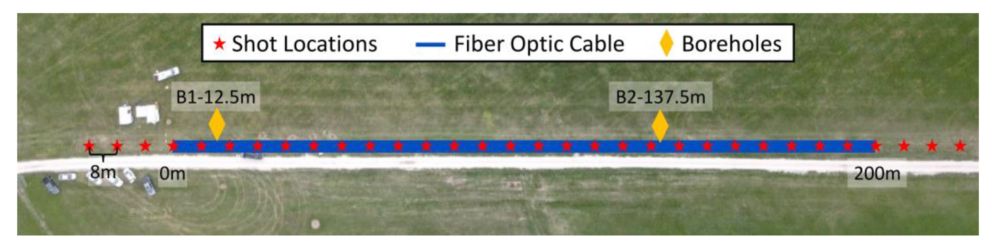
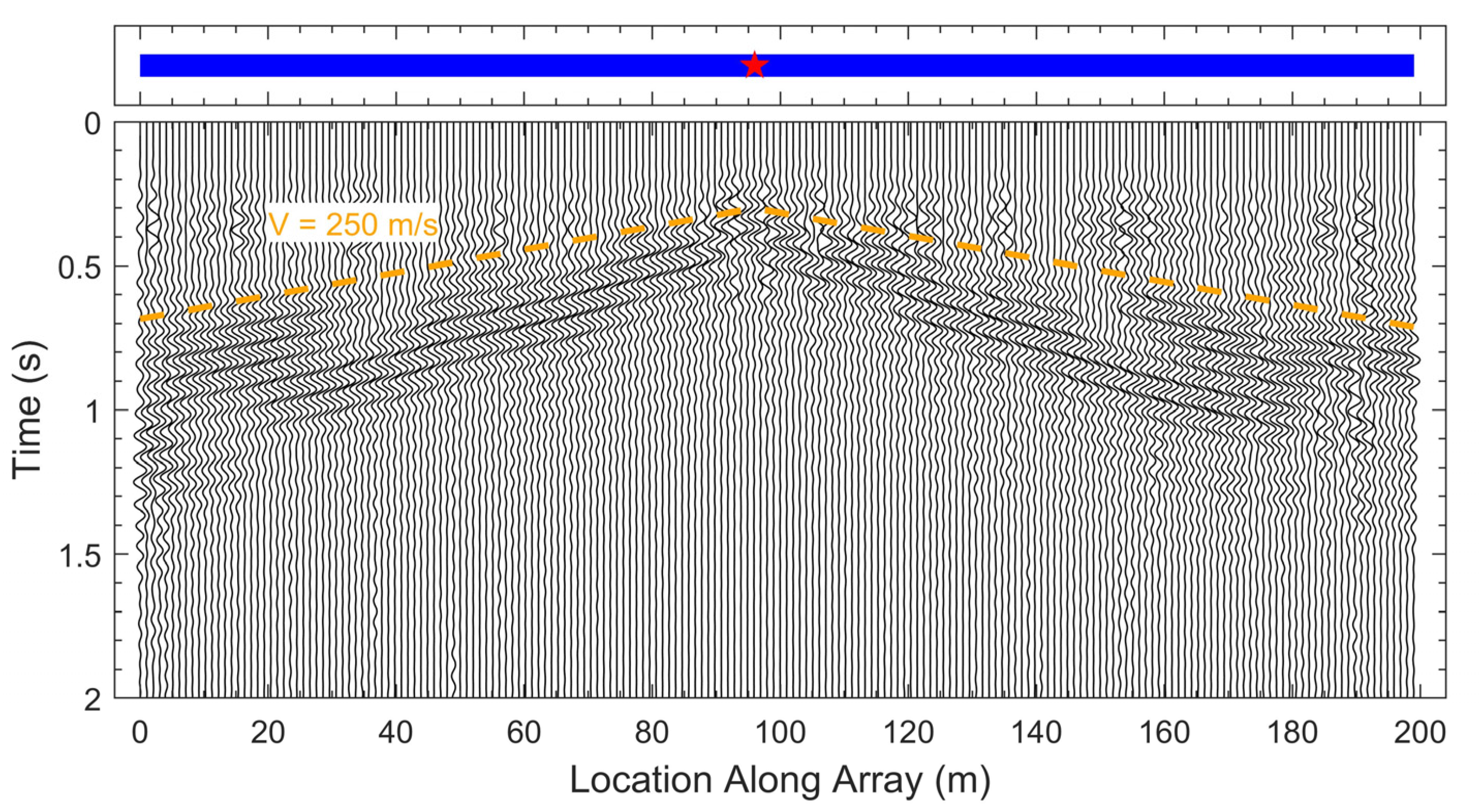
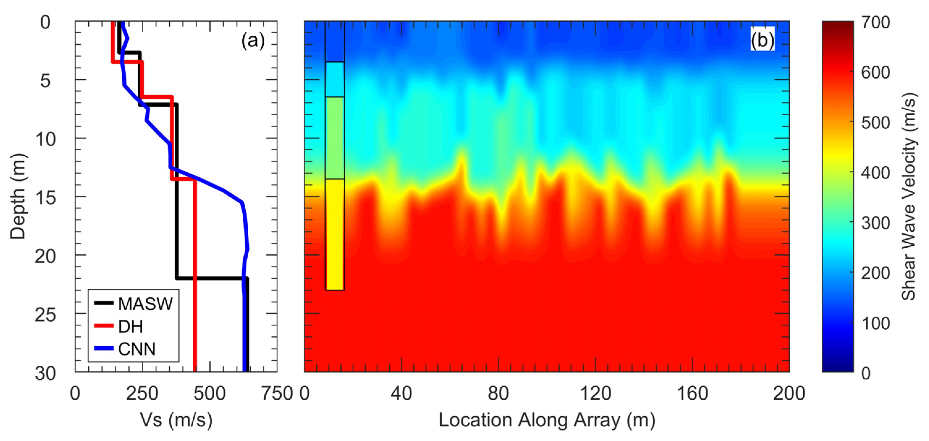
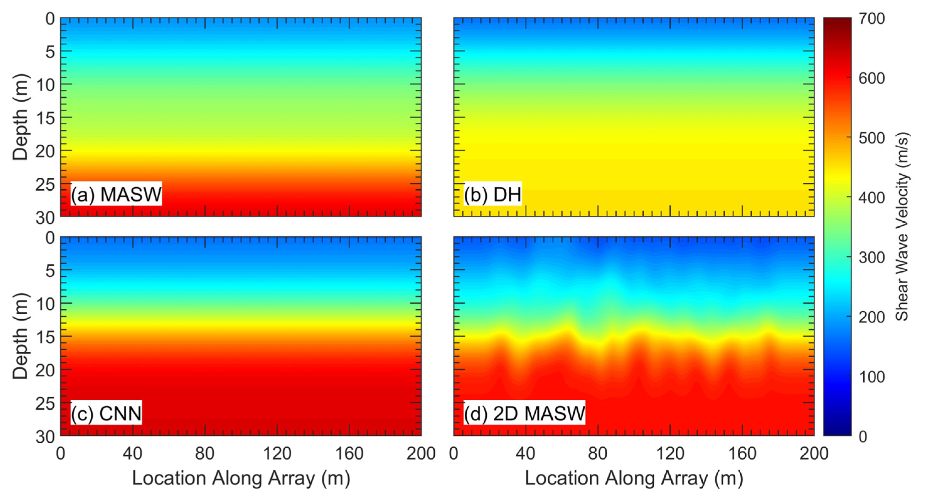
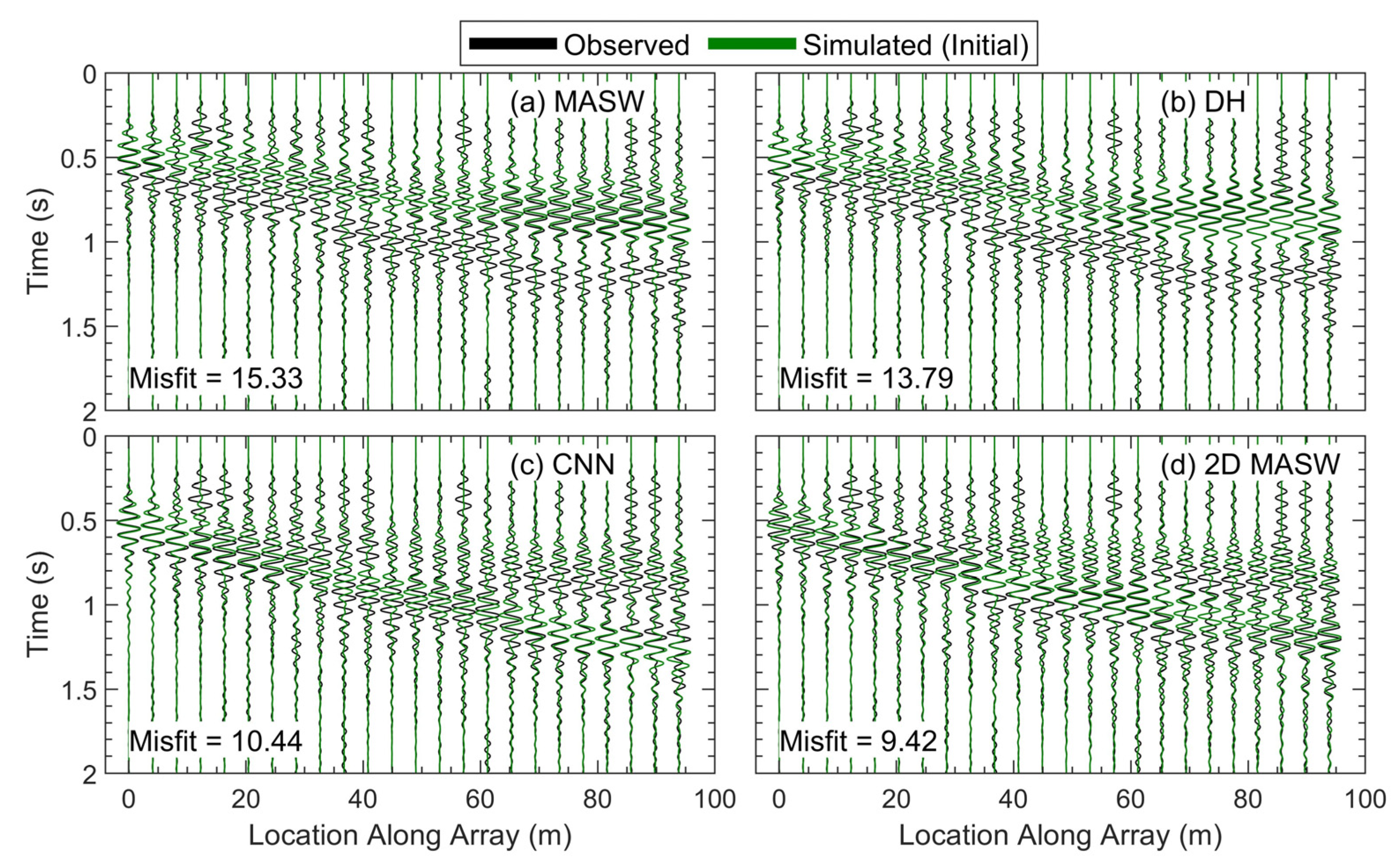
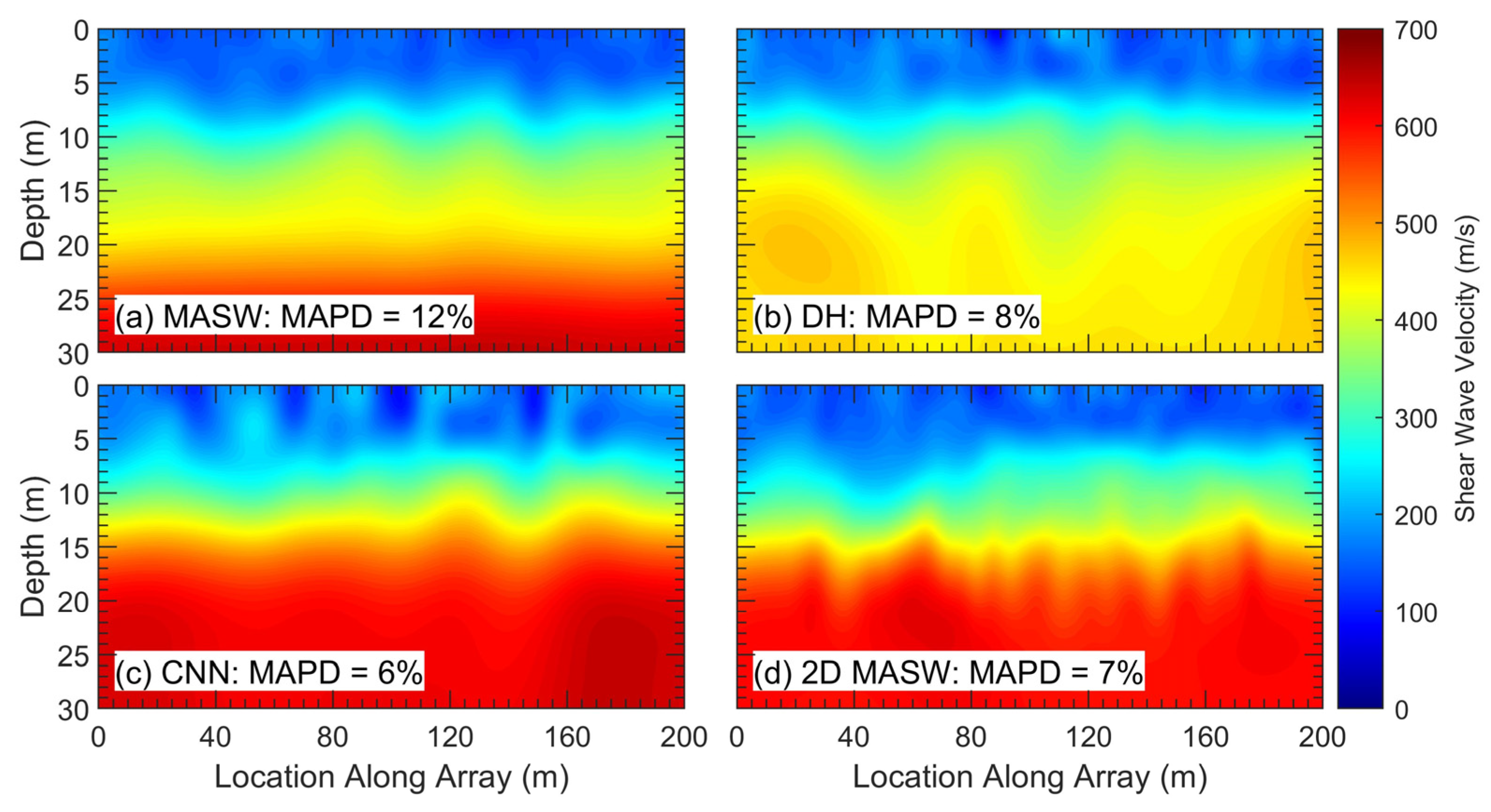
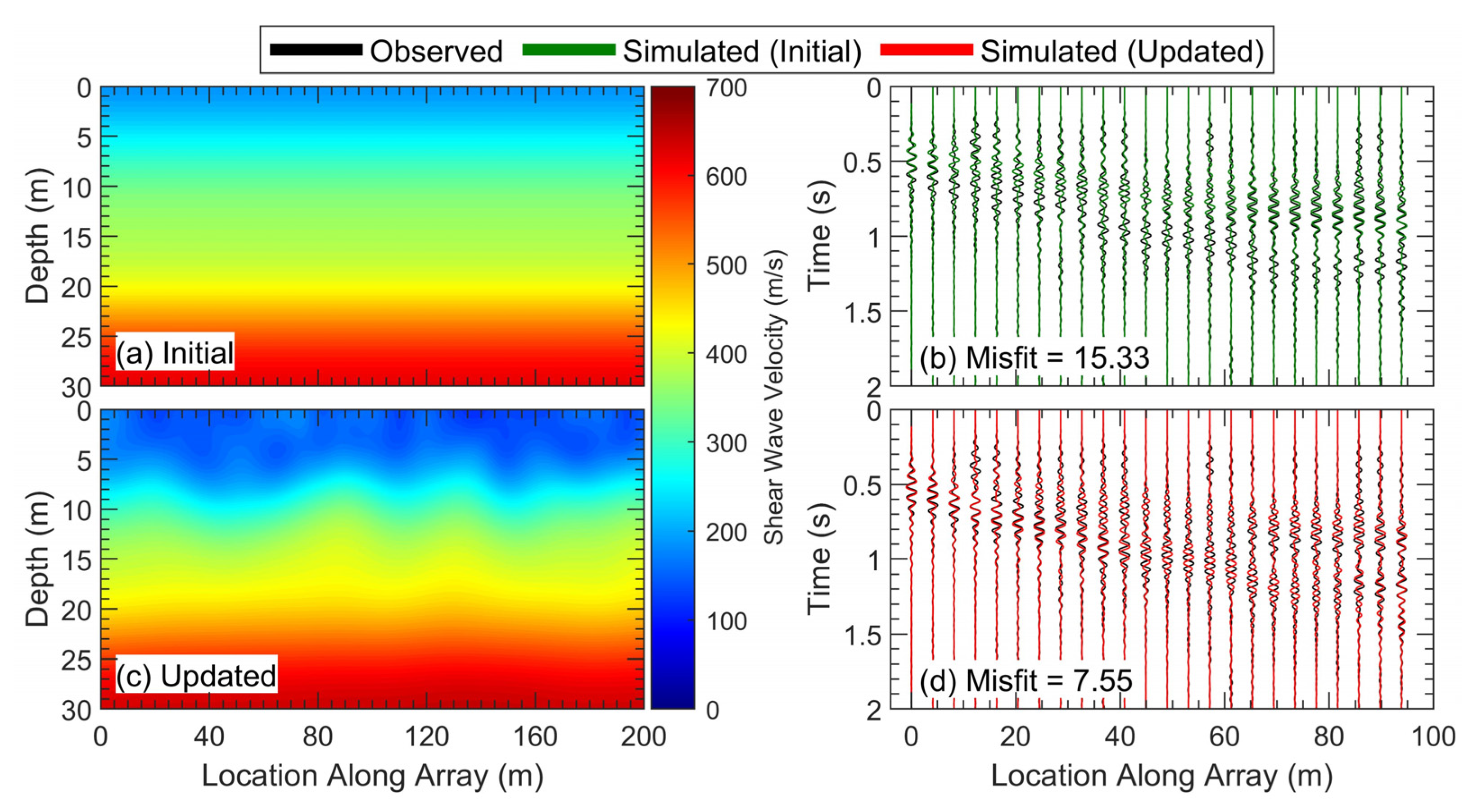
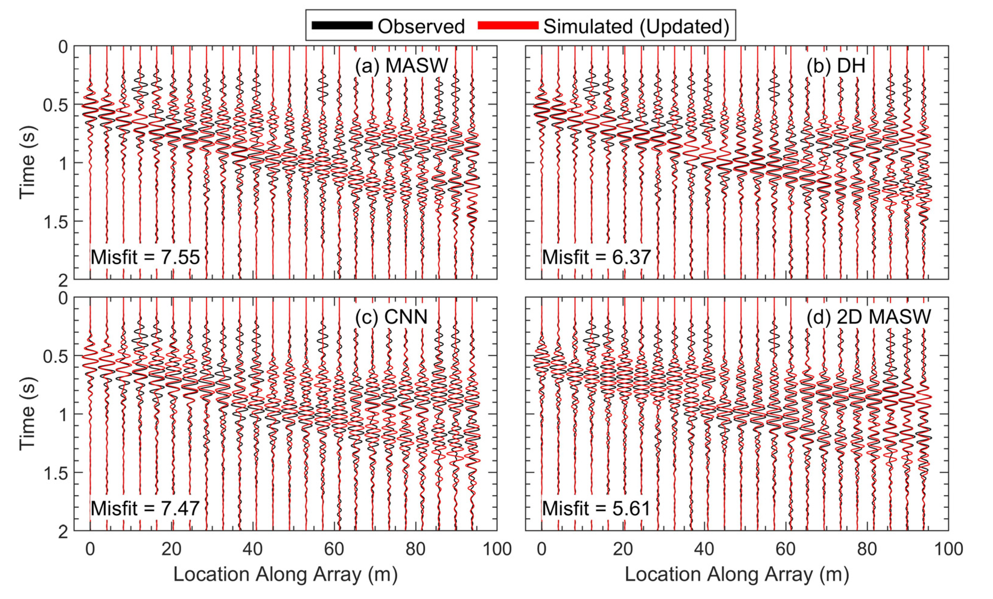
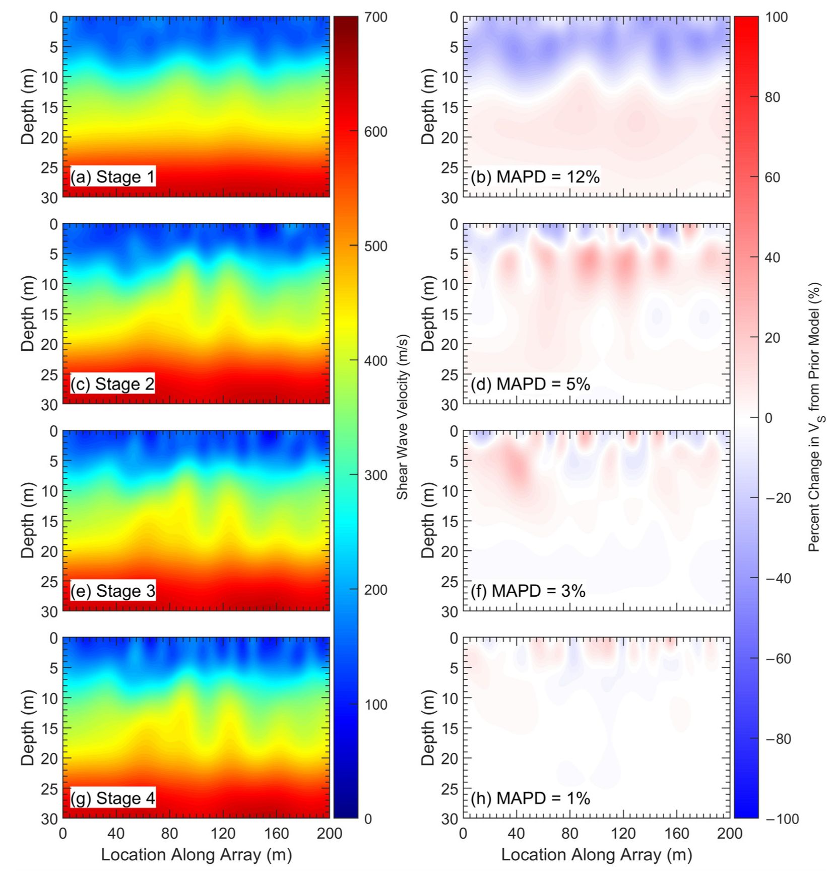
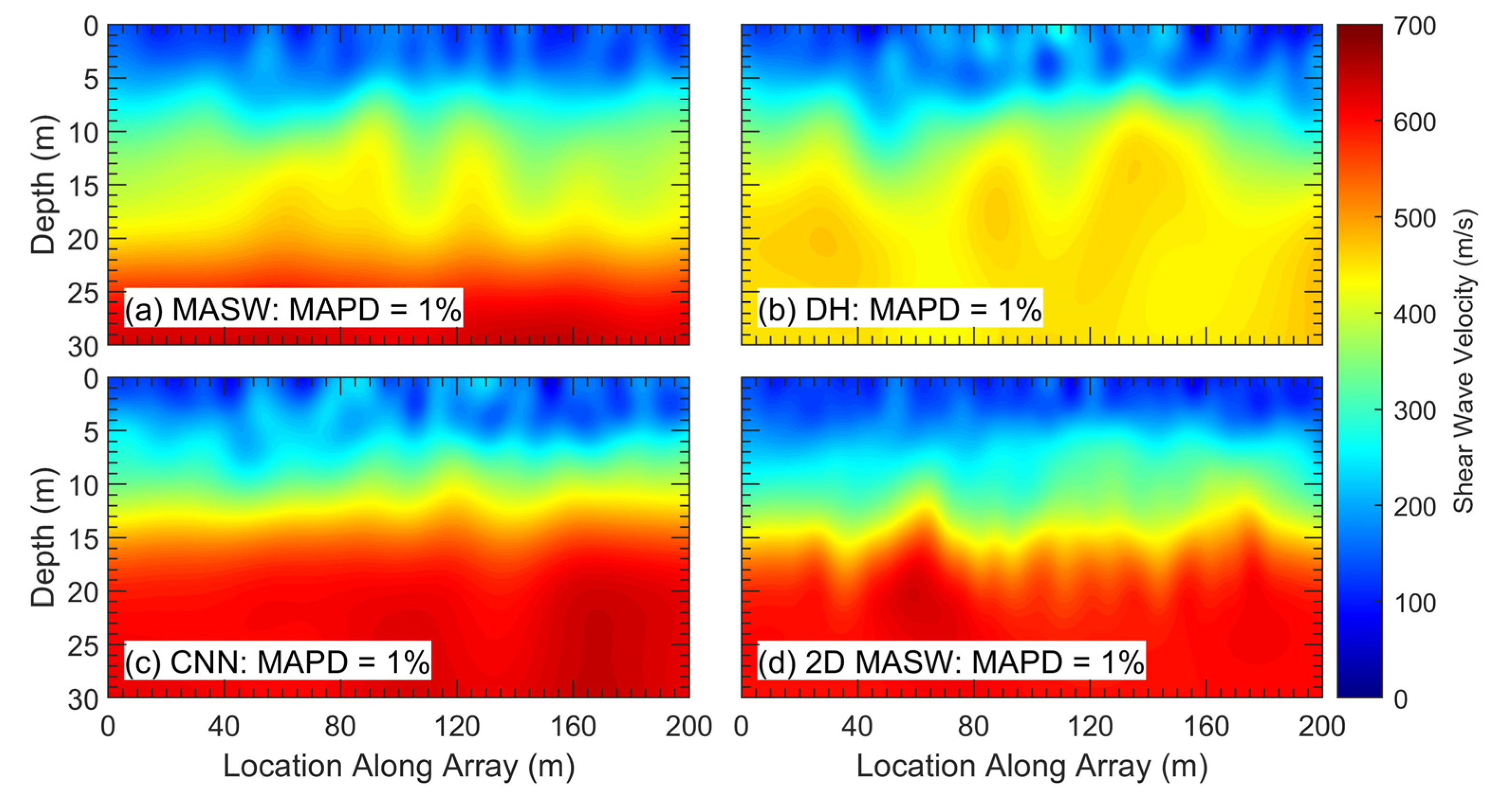
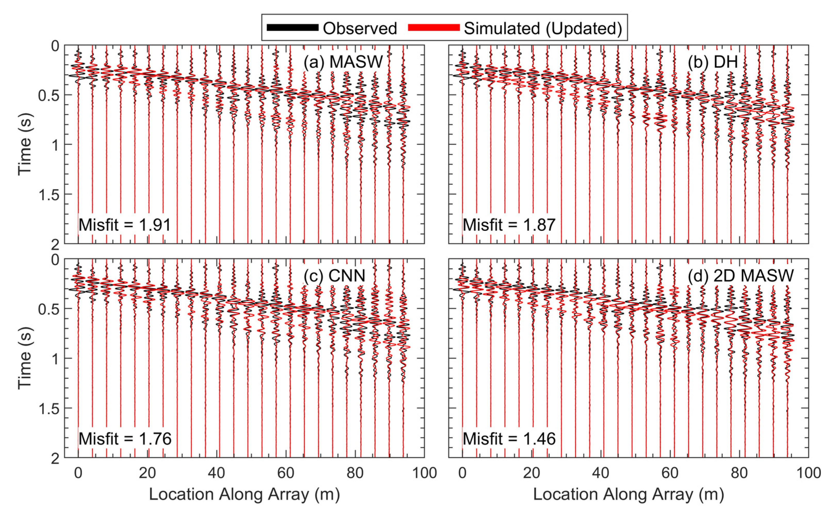
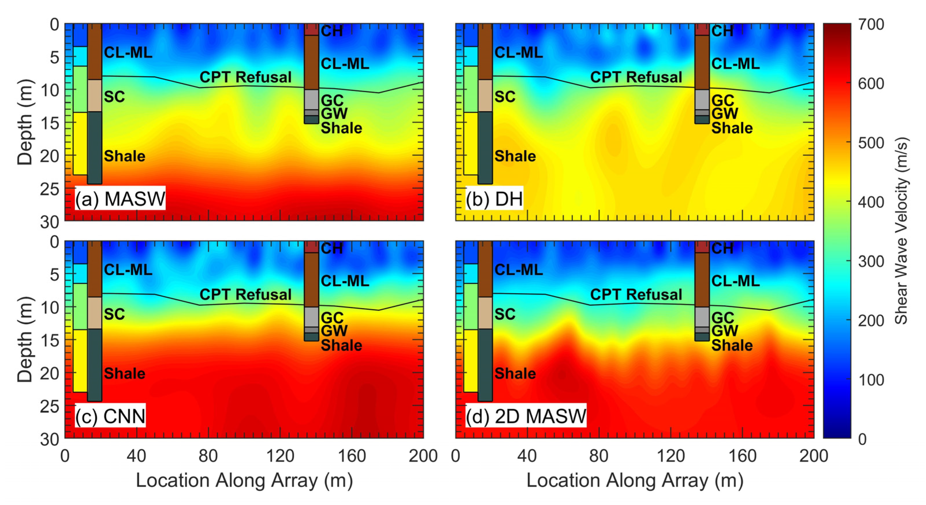9. Conclusions

FWI was performed on DAS data collected at a well-characterized site using four high-quality, but different, site-specific starting models. The DAS data were collected using an approximately 200 m long DAS array and were inverted to obtain 2D V_S images over the entire lateral extent down to a depth of 30 m. The Salvus software suite [50] was used to invert the strain measurements made by the DAS array directly, rather than converting the observed waveforms to particle velocity or displacement, as has been performed in most previous near-surface applications of FWI to DAS data. While the large amount of data provided by DAS (e.g., 95 to 157 channels for each shot used in this study) provides significantly more information for the inversions than would be possible over the same scale with a traditional geophone array, it also requires more computation resources to process on top of the existing need to consider uncertainty resulting from different FWI starting models. Despite this potential challenge, FWI applied to DAS data still has significant potential as a powerful tool for near-surface site characterization. FWI results based on all four starting models were able to match the major features of the observed DAS waveforms well, with similar levels of waveform misfit across the results from all four starting models. The final 2D V_S images obtained from all four starting models agreed reasonably well over the top 10 m of the subsurface; however, only two out of the four starting models produced 2D V_S images that both compared well with one another across the entire depth range and agreed well with subsurface layering from borehole lithology logs at the site. Thus, while the choice of starting model was demonstrated to be a significant source of uncertainty in the FWI results, comparing the V_S images resulting from various high-quality, site-specific starting models can also indicate which portions of the final inverted subsurface model(s) can be used with confidence and which cannot. There are a large number of factors affecting the FWI inversions discussed in this study, including model attenuation assumptions, point-to-line source conversions, idealized source forcing function, choice of gradient smoothing, and optimization configuration. While these factors could theoretically be varied or inverted to more fully account for uncertainty, this practically presents a challenge due to the need to devote significant computational resources to FWI. As such, additional future studies are required to more fully investigate the use of DAS for FWI and to more fully assess uncertainties associated with the starting model and other critical factors, such as depth-dependent FWI non-uniqueness, which is most certainly site-specific and linked to waveform bandwidth.