

Geocryological Structure of a Giant Spring Aufeis Glade at the Anmangynda River (Northeastern Russia)

Abstract
:
1. Introduction
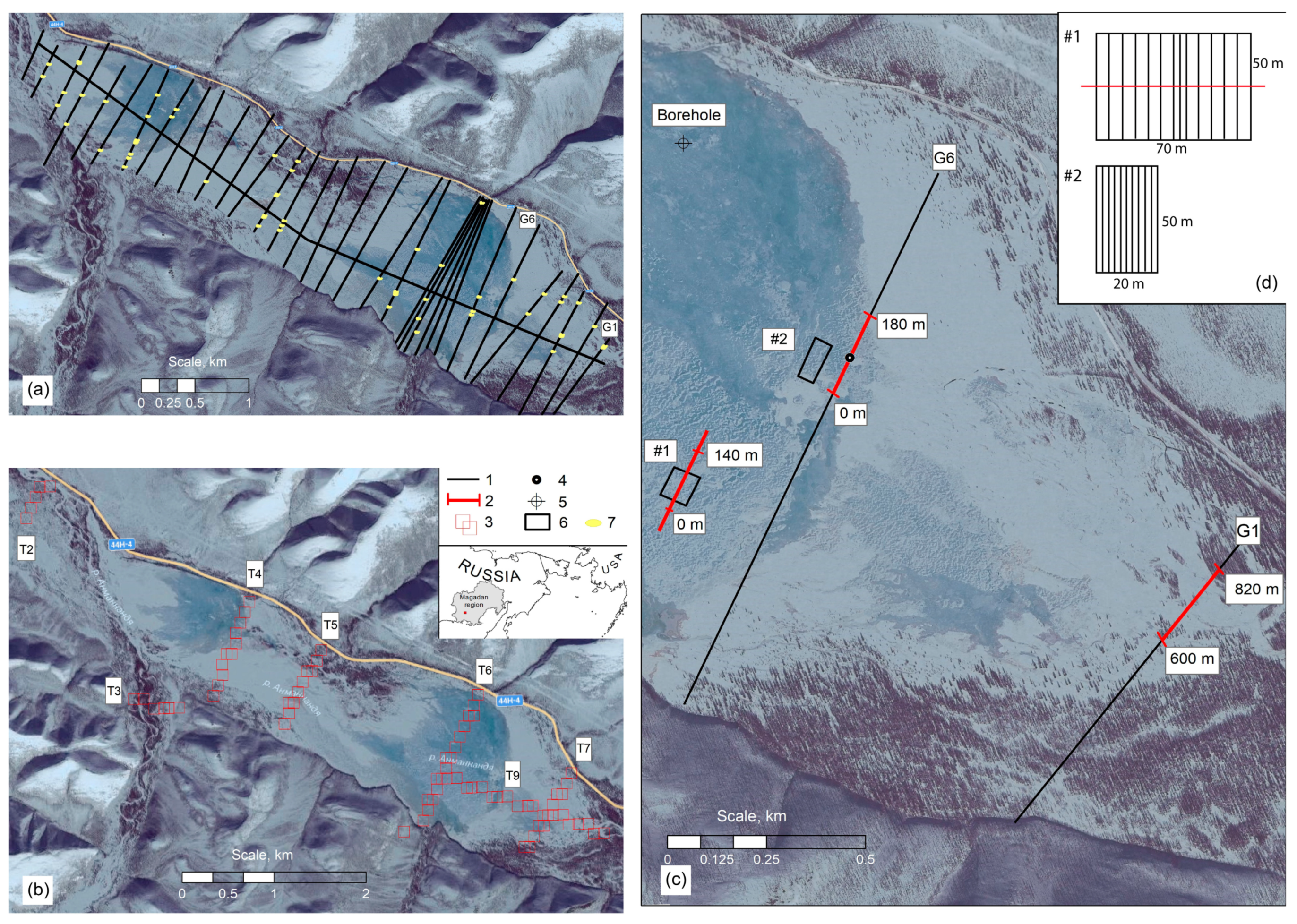
2. Study Area
3. Materials and Methods
3.1. GPR Surveys
3.2. Capacitively Coupled Electrical Resistivity Tomography (CCERT)
3.3. Transient Electromagnetic (TEM) Method
3.4. Thermometric and Hydrogeological Monitoring at the Aufeis Field
4. Results and Interpretation
4.1. Distribution of Ice Thickness and Aufeis Volume
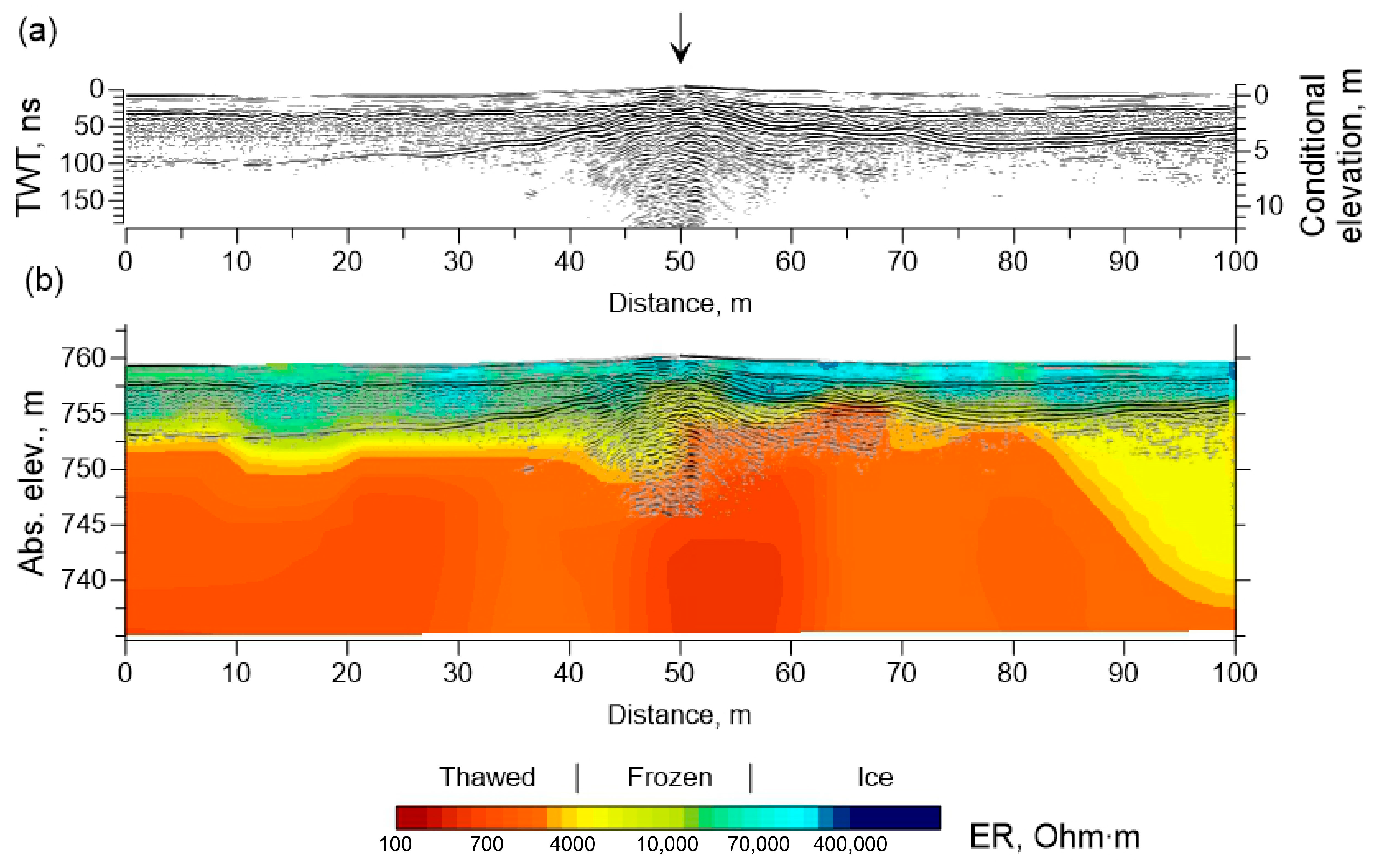
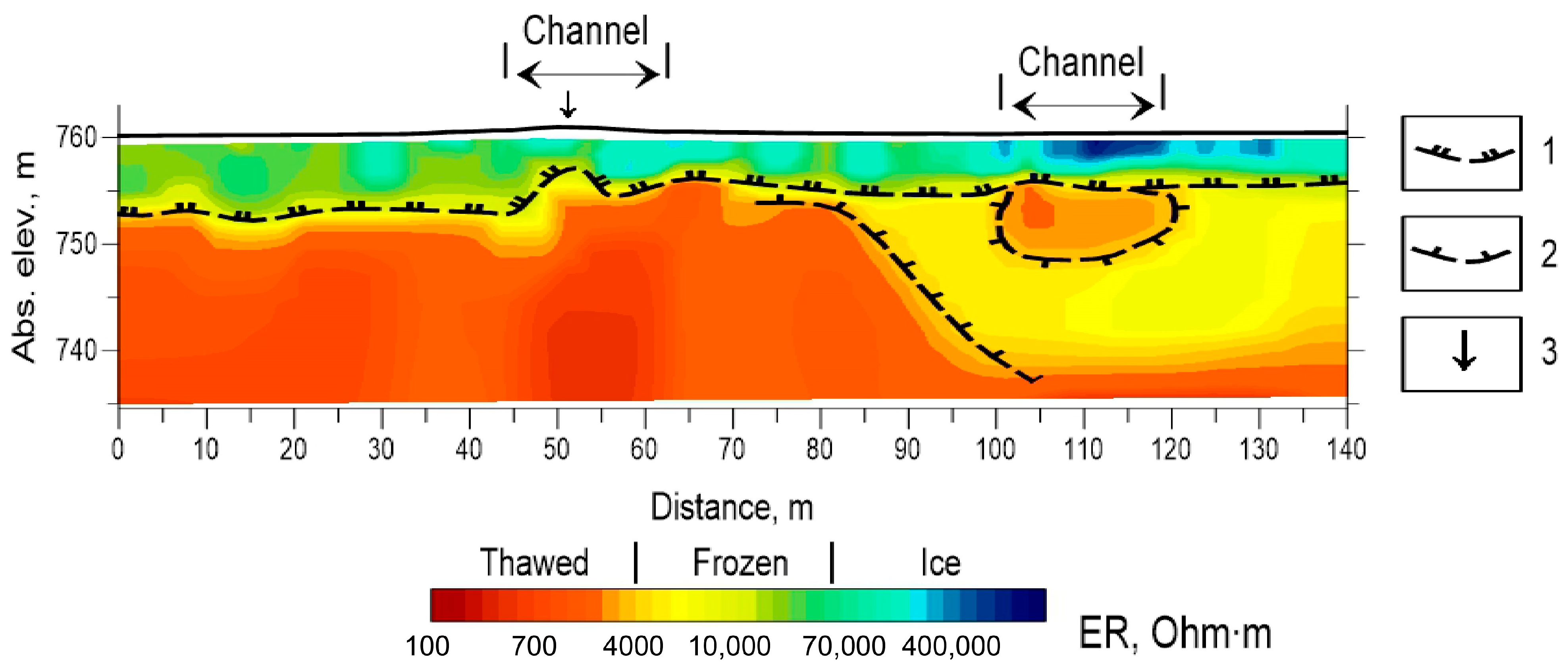
4.2. Investigation of the Areas of the GW Springs Discharging under the Ice
4.3. The Structure of GW Spring Discharging from the Frost Mound
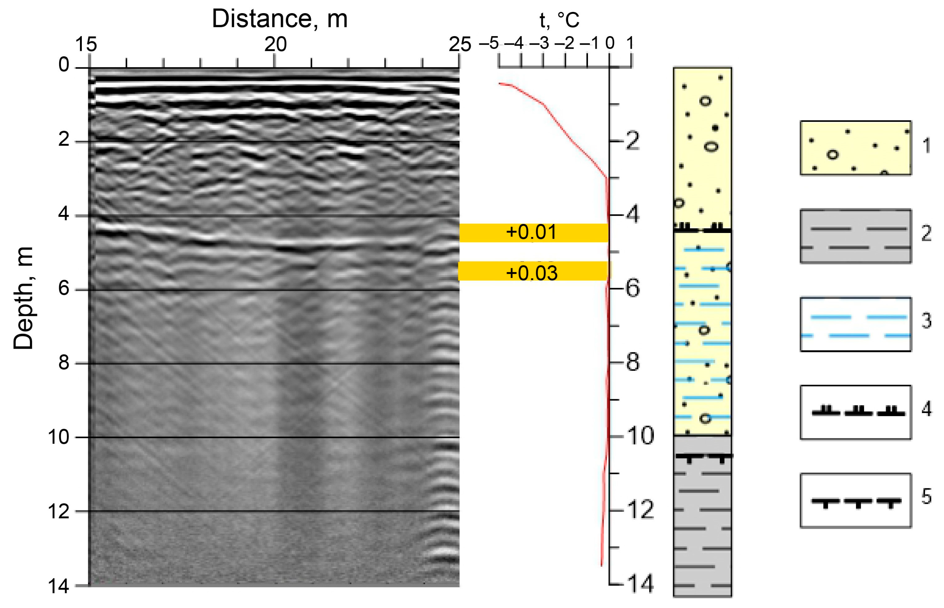
4.4. Seasonal Freezing along the River Channel and the Formation of Water Lenses inside the Ice
4.5. Investigation of the Geology Structure of the Aufeis Glade Based on TEM Results
5. Discussion
6. Conclusions
Supplementary Materials
Author Contributions
Funding
Data Availability Statement
Acknowledgments
Conflicts of Interest
References
- Ensom, T.P.; Makarieva, O.M.; Morse, P.D.; Kane, D.L.; Alekseev, V.R.; Marsh, P. The distribution and dynamics of aufeis in permafrost regions. Permafr. Periglac. Process. 2020, 31, 383–395. [Google Scholar] [CrossRef]
- Morse, P.; Wolfe, S. Long-Term River icing dynamics in discontinuous permafrost, subarctic Canadian Shield: River icing dynamics in discontinuous permafrost, subarctic Canada. Permafr. Periglac. Process. 2016, 28, 580–586. [Google Scholar] [CrossRef]
- Brombierstäudl, D.; Schmidt, S.; Nüsser, M. Distribution and relevance of Aufeis (icing) in the upper Indus Basin. Sci. Total Environ. 2021, 780, 146604. [Google Scholar] [CrossRef] [PubMed]
- Makarieva, O.; Nesterova, N.; Shikhov, A.; Zemlianskova, A.; Luo, D.; Ostashov, A.; Alexeev, V. Giant Aufeis—Unknown Glaciation in North-Eastern Eurasia According to Landsat Images 2013–2019. Remote Sens. 2022, 14, 4248. [Google Scholar] [CrossRef]
- Turcotte, B.; Dubnick, A.; McKillop, R.; Ensom, T. Icing and aufeis in cold regions I: The origin of overflow. Can. J. Civil Eng. 2023. e-First. [Google Scholar] [CrossRef]
- Romanovsky, N.N. Underground Waters in Cryolithozone; Moscow State University: Moscow, Russia, 1983; 231p. (In Russian) [Google Scholar]
- Gavrilova, M.K. Changes in the current climate in the permafrost region in Asia. In Overview of the State and Trends of Climate Change in Yakutia; SB RAS: Yakutia, Russia, 2003; pp. 13–18. (In Russian) [Google Scholar]
- Pomortsev, O.A.; Kashkarov, E.P.; Popov, V.F. Aufeis: Global warming and processes of aufeis formation (rhythmic basis of long-term prognosis). Bull. Yakutsk. State Univ. 2010, 7, 40–48. (In Russian) [Google Scholar]
- Alekseev, V.R.; Makarieva, O.M.; Shikhov, A.N.; Nesterova, N.V.; Ostashov, A.A.; Zemlyanskova, A.A. Atlas of Giant Aufeis-Taryn of the North-East of Russia; SB RAS: Novosibirsk, Russia, 2021; 302p, ISBN 978-5-6046428-2-5. (In Russian) [Google Scholar]
- Zonov, B.N. Aufeis and polynyas in the rivers of the Yana-Kolyma upland. In Transactions of the Obruchev Permafrost Institute of the USSR Academy of Sciences; Publishing House of the USSR Academy of Science: Moscow, Russia, 1944; Volume 44, pp. 33–92. (In Russian) [Google Scholar]
- Shvetsov, P.F. Groundwater of the Verkhoyansk-Kolyma Folded Area and Specific Features of Its Manifestation Related to Low Permafrost Temperatures; Publishing House of the USSR Academy of Science: Moscow, Russia, 1951; 279p. (In Russian) [Google Scholar]
- Koreisha, M.M. Some features of the study of glaciers and aufeis in the North-East of the USSR. Data Glaciol. Stud. 1972, 19, 245–247. (In Russian) [Google Scholar]
- Kane, D.L.; Slaughter, C. Seasonal regime and hydrological significance of stream icings in central Alaska. In Role of Snow and Ice in Hydrology: Proceedings of the Banff Symposia; Unesco-WMO-IAHS: Montpellier, France, 1973; Volume 1, pp. 528–540. [Google Scholar]
- Yoshikawa, K.; Hinzman, L.D.; Kane, D.L. Spring and aufeis (icing) hydrology in Brooks Range, Alaska. J. Geophys. Res. Space Phys. 2007, 112, 1–14. [Google Scholar] [CrossRef]
- Carey, K.L. Icings developed from surface water and ground water. In Cold Regions Science and Engineering Monograph III-D3; U.S. Army Cold Regions Research and Engineering Laboratory: Hanover, NH, USA, 1973. [Google Scholar]
- Liu, W.; Fortier, R.; Molson, J.; Lemieux, J.-M. A Conceptual Model for Talik Dynamics and Icing Formation in a River Floodplain in the Continuous Permafrost Zone at Salluit, Nunavik (Quebec), Canada. Permafr. Periglac. Process. 2021, 32, 468–483. [Google Scholar] [CrossRef]
- Terry, N.; Grunewald, E.; Briggs, M.; Gooseff, M.; Huryn, A.D.; Kass, M.A.; Tape, K.D.; Hendrickson, P.; Lane, J.W., Jr. Seasonal Subsurface Thaw Dynamics of an Aufeis Feature Inferred from Geophysical Methods. J. Geophys. Res. Earth Surf. 2020, 125, e2019JF005345. [Google Scholar] [CrossRef]
- Kolyma Territorial Administration for Hydrometeorological and Environmental Monitoring. Report on the Results of the Water Balance Studies with the Aufeis Component in the Anmangynda River Basin; Kolyma Territorial Administration for Hydrometeorological and Environmental Monitoring: Magadan, Russia, 1977; 62p. (In Russian) [Google Scholar]
- Tolstikhin, O.N. Icings and Ground Waters of North-East of USSR; Nauka: Novosibirsk, Russia, 1974; 164p. (In Russian) [Google Scholar]
- Bukaev, N.A. Main Peculiarities of Regime of Giant Aufeis in the upper Part of Kolyma River (the Anmangynda Aufeis as an Example); Aufeis of Siberia; Nauka: Moscow, Russia, 1969; pp. 62–78. (In Russian) [Google Scholar]
- USSR State Committee for Hydrometeorology and Environmental Control. State Water Cadastre: Main hydrological Characteristics (for 1971–1975 and the Whole Period of Observation); 19 (North-East); Gidrometeoizdat: Leningrad, Russia, 1978. (In Russian) [Google Scholar]
- Pavlyuchenko, L.A. Geological Map of the USSR. Verkhnekolymskaya Series. Scale 1:200000. Sheet P-55-XXX. Explanatory Note; Nedra: Moscow, Russia, 1968; 67p. (In Russian) [Google Scholar]
- Tolstikhin, O.N. Hydrogeology of the USSR. Volume XXVI. North-East of the USSR; Nedra: Moscow, Russia, 1972; 297p. (In Russian) [Google Scholar]
- Alekseev, V.R.; Boyarintsev, E.L.; Dovbysh, V.N. Long-term dynamics of dimensions of the Amangynda aufeis in the conditions of climate change. In Proceeding of the All-Russia Scientific Conference Devoted to the Memory of A.V. Rozhdestvensky, Outstanding Hydrology Researcher “Current Problems of Stochastic Hydrology and Runoff Regulation”, Moscow, Russia, 10–12 April 2012; pp. 298–305. (In Russian). [Google Scholar]
- Zemlianskova, A.A.; Alekseev, V.R.; Shikhov, A.N.; Ostashov, A.A.; Nesterova, N.V.; Makarieva, O.M. Long-term dynamics of the huge Anmangynda aufeis in the North-East of Russia (1962–2021). Led I Sneg. Ice Snow 2023, 63, 71–84. (In Russian) [Google Scholar] [CrossRef]
- Logical Systems Company. Radio Engineering Device for Subsurface Sensing (Georadar) “OKO-3”. TECHNICAL Description. Operating Instructions; LLC “LOGICAL SYSTEMS”: Moscow, Russia, 2018; 42p. [Google Scholar]
- Geoscan32 Software. Available online: https://www.geotech.ru/programmnoe_obespechenie_geoscan32/ (accessed on 25 May 2023).
- Glen, J.W.; Paren, J.G. The electrical properties of snow ice. J. Glaciol. 1975, 151, 15–37. [Google Scholar] [CrossRef]
- Gruzdev, A.I.; Bobachev, A.A.; Shevnin, V.A. The determination of usability area for capacitive resistivity measurements. Mosc. Univ. Bull. 2020, 4, 100–106. (In Russian) [Google Scholar] [CrossRef]
- High-Frequency Electrical Exploration Station “VEGA”. Available online: https://www.geotech.ru/vega/ (accessed on 25 May 2023).
- Loke, M.H. Tutorial: 2-D and 3-D Electrical Imaging Surveys; Geotomo Software: Penang, Malaysia, 2014; 216p. [Google Scholar]
- FastSnap Digital Electrical Survey Station. Operation and Software Manual; Sigma-Geo LLC: Irkutsk, Russia, 2017; 177p. [Google Scholar]
- Impedans Company and in Temp Data Loggers. Available online: https://impedance-bio.ru/ (accessed on 25 May 2023).
- Zemlianskova, A.; Makarieva, O.; Shikhov, A.; Alekseev, V.; Nesterova, N.; Ostashov, A. The impact of climate change on seasonal glaciation in the mountainous permafrost of North-Eastern Eurasia by the example of the giant Anmangynda aufeis. CATENA 2023, 233, 107530. [Google Scholar] [CrossRef]
- Onset HOBO and in Temp Data Loggers. Available online: https://www.onsetcomp.com/ (accessed on 25 May 2023).
- Olenchenko, V.V.; Gagarin, L.A.; Khristoforov, I.I.; Kolesnikov, A.B.; Efremov, V.S. The Structure of a Site with Thermo-Suffosion Processes within Bestyakh Terrace of the Lena River, according to Geophysical Data. Earth’s Cryosphere 2017, XXI, 14–23. [Google Scholar] [CrossRef]
- Lebedev, V.M. Monitoring of Aufeis in the Anmangynda River Basin. Magadan GMO Collect. Work. 1969, 2, 122–137. (In Russian) [Google Scholar]
- Lebedev, V.; Ipateva, A. Anmangynda Aufeis, Its Regime and Role in Water Balance of the River Basin. Tr. Dvnigmi 1980, 84, 86–93. (In Russian) [Google Scholar]
- Mikhailov, V.M. Through taliks in the valleys of small rivers. Kolyma 2001, 4, 31–34. (In Russian) [Google Scholar]
- Solovyova, G.V. Aufeis Regulation of Groundwater Runoff in the Areas of Widespread Occurrence of Permafrost; Final Report; VSEGINGEO: Moscow, Russia, 1967; Volume 1, 447p. (In Russian) [Google Scholar]


Disclaimer/Publisher’s Note: The statements, opinions and data contained in all publications are solely those of the individual author(s) and contributor(s) and not of MDPI and/or the editor(s). MDPI and/or the editor(s) disclaim responsibility for any injury to people or property resulting from any ideas, methods, instructions or products referred to in the content. |
© 2023 by the authors. Licensee MDPI, Basel, Switzerland. This article is an open access article distributed under the terms and conditions of the Creative Commons Attribution (CC BY) license (https://creativecommons.org/licenses/by/4.0/).
Share and Cite
Olenchenko, V.; Zemlianskova, A.; Makarieva, O.; Potapov, V. Geocryological Structure of a Giant Spring Aufeis Glade at the Anmangynda River (Northeastern Russia). Geosciences 2023, 13, 328. https://doi.org/10.3390/geosciences13110328
Olenchenko V, Zemlianskova A, Makarieva O, Potapov V. Geocryological Structure of a Giant Spring Aufeis Glade at the Anmangynda River (Northeastern Russia). Geosciences. 2023; 13(11):328. https://doi.org/10.3390/geosciences13110328
Chicago/Turabian StyleOlenchenko, Vladimir, Anastasiia Zemlianskova, Olga Makarieva, and Vladimir Potapov. 2023. "Geocryological Structure of a Giant Spring Aufeis Glade at the Anmangynda River (Northeastern Russia)" Geosciences 13, no. 11: 328. https://doi.org/10.3390/geosciences13110328