
Soil Formation and Mass Redistribution during the Holocene Using Meteoric 10Be, Soil Chemistry and Mineralogy

 , , , and
Abstract
:1. Introduction
2. Site Descriptions
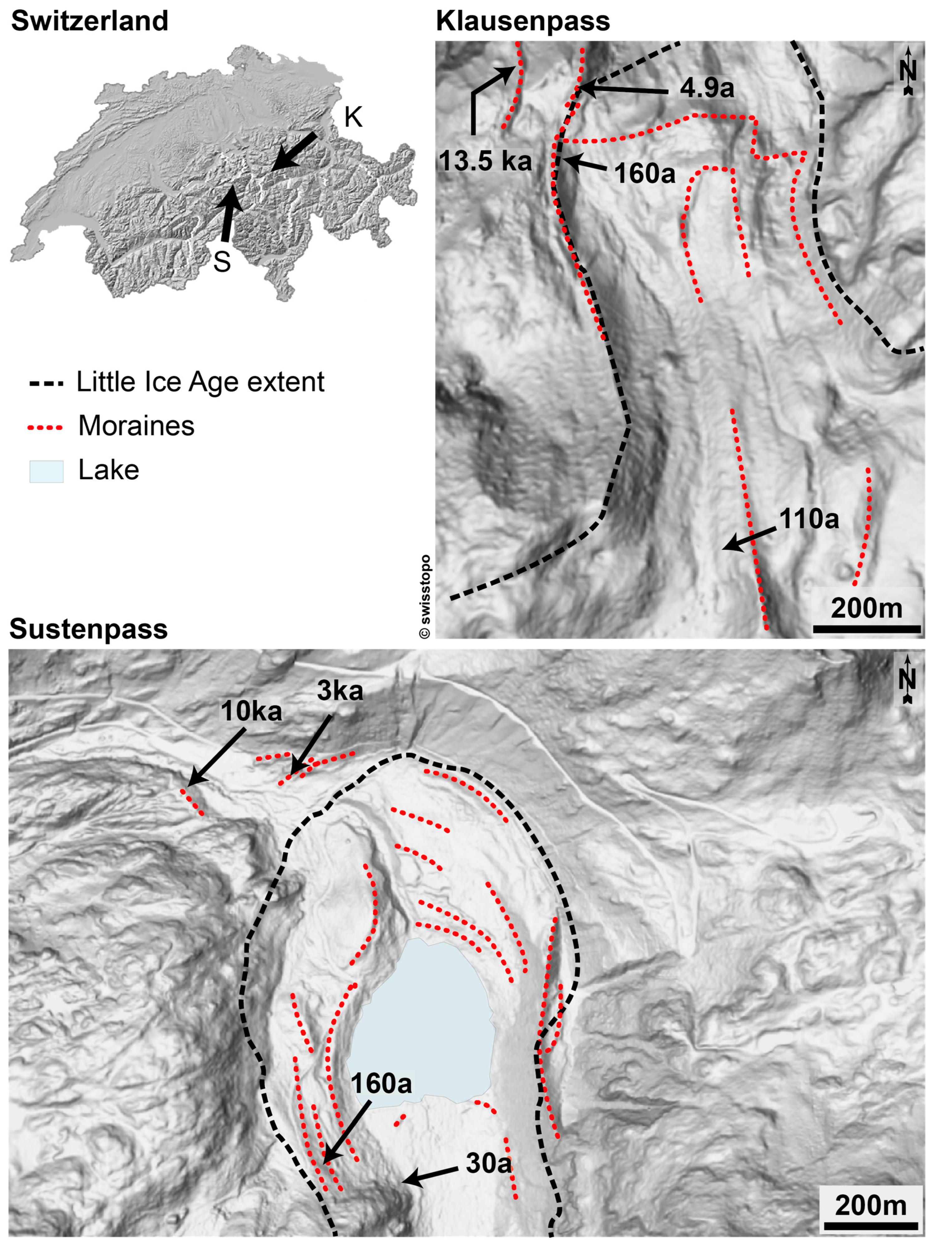
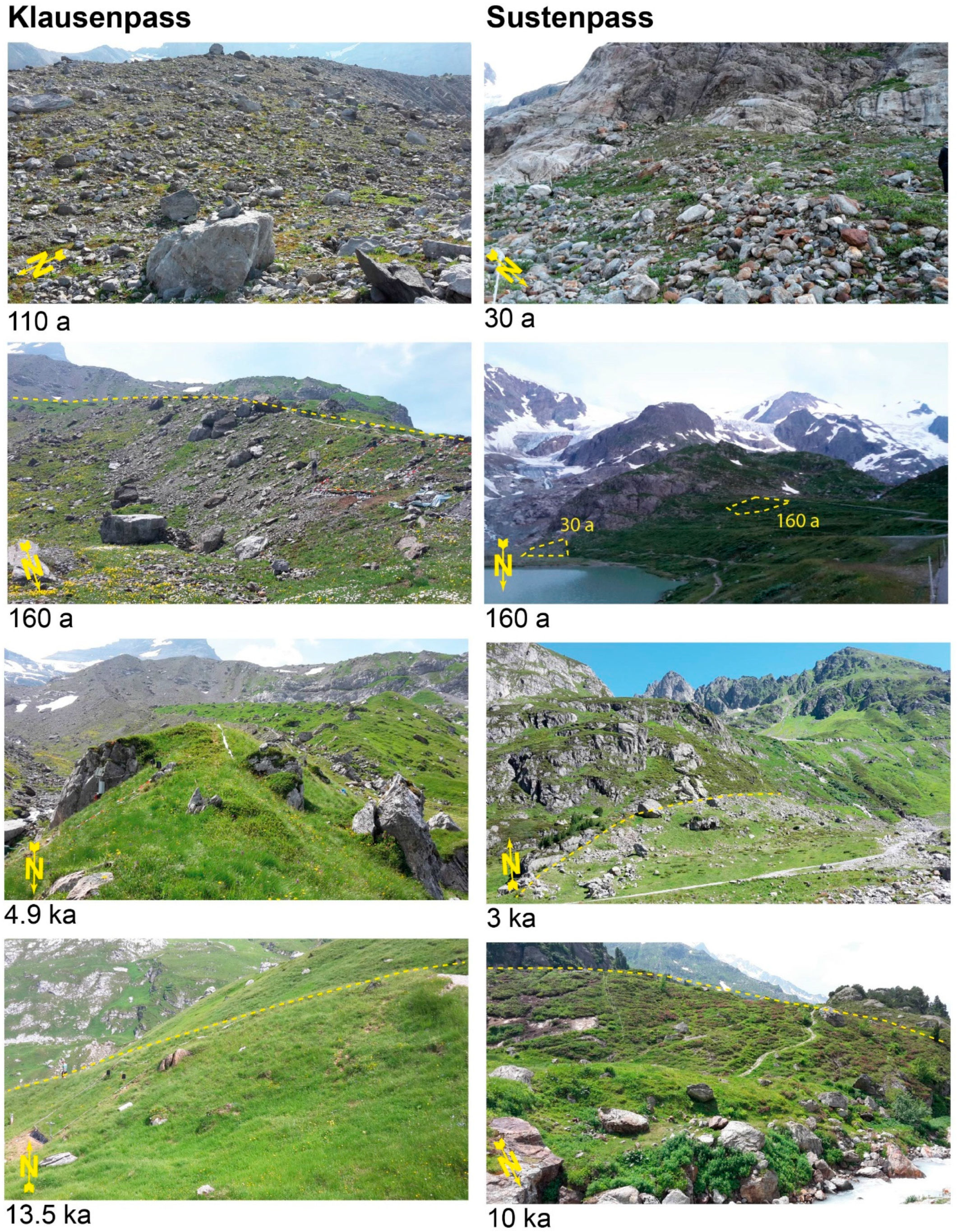
2.1. Klausenpass
2.2. Sustenpass

| Soil Profile | Surface Age | Aspect | Slope | Elevation | Vegetation | Soil Type | Horizon | Depth | Bulk Density | Skeleton | pH (CaCl2) | LOI |
|---|---|---|---|---|---|---|---|---|---|---|---|---|
| (years) | (deg) | (m a.s.l.) | (Dominating Species) | (cm) | (g cm−3) | (wt. %) | (%) | |||||
| K-A1 | 110 | WNW | 27 | 2200 | Saxifraga aizoides dominated stocks | Hyperskeletic Leptosol | C1 | 0–10 | 1.8 ± 0.1 | 62 | 7.8 | 1.8 |
| C2 | 10–20+ | 1.4 ± 0.5 | 61.2 | 7.6 | 2 | |||||||
| K-A2 | 110 | WNW | 27 | 2200 | Initial snowbed communities of type Arabidion caeruleae | Hyperskeletic Leptosol | C1 | 0–10 | 1.5 ± 0.2 | 68.3 | 7.7 | 1.9 |
| C2 | 10–20+ | 1.3 ± 0.6 | 67.6 | 7.6 | 1.8 | |||||||
| K-B1 | 160 | NE | 31 | 2030 | Thlaspietum rotundifolii | Hyperskeletic Leptosol | AC | 0–15 | 1.2 ± 0.4 | 71.6 | 7.3 | 8.4 |
| C | 15–25+ | 0.7 ± 0.1 | 74.5 | 7.8 | 3.3 | |||||||
| K-B2 | 160 | NE | 31 | 2030 | Dryadetum octopetalae | Hyperskeletic Leptosol | AC | 0–10 | 1.1 ± 0.7 | 68 | 7.5 | 8.9 |
| C | 10–28+ | 0.8 ± 0 | 64.6 | 7.7 | 3.2 | |||||||
| K-C1 | 4900 1 | WNW | 36 | 2020 | Caricetum ferruginei | Calcaric Skeletic Cambisol | A | 0–15 | 0.5 ± 0.1 | 11.3 | 5.8 | 18.7 |
| B | 15–21 | 0.7 ± 0.1 | 64.5 | 7.3 | 10 | |||||||
| BC | 21–60 | 1.5 ± 0.1 | 77.9 | 7.8 | 2.7 | |||||||
| C | 60–80+ | 1.5 ± 0 | 85.3 | 7.7 | 2.2 | |||||||
| K-C2 | 4900 1 | N | 37 | 2010 | Rhododendretum hirsuti | Calcaric Skeletic Cambisol | OA | 0–18 | 0.3 ± 0 | 3.8 | 4.5 | 34.4 |
| B | 18–42 | 0.8 ± 0.1 | 22.7 | 6.7 | 14 | |||||||
| BC | 42–51 | 1.5 ± 0 | 84.6 | 7.8 | 3.8 | |||||||
| C | 51–75+ | 1.7 ± 0.1 | 80.8 | 7.7 | 2.7 | |||||||
| K-D1 | 13,500 2 | NW | 44 | 2000 | Seslerio-Caricetum sempervirentis | Calcaric Skeletic Cambisol | A1 | 0–15 | 0.3 ± 0.1 | 6.9 | 5.9 | 42.4 |
| A2 | 15–28 | 0.5 ± 0 | 40.8 | 6.8 | 20.5 | |||||||
| B | 28–32 | 0.8 ± 0.2 | 73.5 | 7.6 | 5.8 | |||||||
| BC1 | 32–68 | 1.6 ± 0.1 | 75 | 7.8 | 1.64 | |||||||
| BC2 | 68–80+ | 1.7 ± 0.1 | 75 | 7.8 | 1.63 | |||||||
| K-D2 | 13,500 2 | ENE | 32 | 2010 | Caricetum ferruginei | Calcaric Skeletic Cambisol | OE | 0–30 | 0.5 ± 0.1 | 22.8 | 6.6 | 24.5 |
| B | 30–35 | 1.4 ± 0.1 | 74.3 | 7.8 | 2.3 | |||||||
| BC | 35–70+ | 1.9 ± 0.1 | 82.1 | 7.8 | 1.7 | |||||||
| S-A1 | 30 | ENE | 40 | 1950 | Initial grassland vegetation, rich in Trifolium badium/pallescens, Luzula alpino-pilosa | Hyperskeletic Leptosol | AC | 0–10 | 0.9 ± 0.6 | 53.5 | 6.1 | 1.1 |
| C | 10–30+ | 1.5 ± 0.4 | 79.4 | 6.6 | 1.3 | |||||||
| S-A2 | 30 | ENE | 35 | 1950 | Pioneer vegetation at sandy sites, Epilobietum fleischeri subass rhacomitrietosum | Hyperskeletic Leptosol | C | 0–50+ | 0.7 ± 0.4 | 53.2 | 6.7 | 0.8 |
| S-B1 | 160 | ENE | 31 | 1990 | Creeping dwarf shrup patches, high coverage of Salix retusa | Hyperskeletic Leptosol | OA | 0–10 | 1.7 ± 0.1 | 59.4 | 4.7 | 4.4 |
| AC | 10–20 | 1.8 ± 0.1 | 57.4 | 4.8 | 1.7 | |||||||
| C1 | 20–40 | 1.9 ± 0 | 56 | 4.8 | 1.3 | |||||||
| C2 | 40–55+ | 1.6 ± 0.3 | 42.3 | 5.1 | 1.1 | |||||||
| S-B2 | 160 | NE | 28 | 1990 | Grassland of the type Poion alpinae | Hyperskeletic Leptosol | A | 0–10 | 1.5 ± 0.3 | 42.7 | 5.5 | 38.4 |
| C1 | 10–30 | 1.9 ± 0.2 | 56.9 | 4.7 | 1.8 | |||||||
| C2 | 30–45+ | 1.8 ± 0.2 | 70.8 | 5 | 1.5 | |||||||
| S-C1 | 3000 | SW | 25 | 1890 | Agrostio rupestris-Sempervivetum montani | Skeletic Cambisol | A | 0–10 | 1.3 ± 0.1 | 50.4 | 4.6 | 3.4 |
| B | 10–30 | 1.5 ± 0.2 | 68.9 | 4.6 | 2.8 | |||||||
| BC | 30–55+ | 1.9 ± 0 | 63.4 | 5.3 | 1.9 | |||||||
| S-C2 | 3000 | S | 24 | 1910 | Carici sempervirentis | Skeletic Cambisol | A | 0–23 | 1 ± 0.5 | 72.2 | 5 | 22.5 |
| Bw | 23–40 | 1.5 ± 0.3 | 81.2 | 5.6 | 13 | |||||||
| BC | 40–60+ | 1.7 ± 0.1 | 79.5 | 6.1 | 2.4 | |||||||
| S-D1 | 10,000 | N | 22 | 1880 | Geo montani-Nardetum | Entic Podzol | O | 0–20 | 0.7 ± 0.5 | 74.4 | 3.4 | 44 |
| OE | 20–36 | 0.7 ± 0.2 | 47.9 | 3.6 | 28.7 | |||||||
| Bs | 36–63 | 1.3 ± 0.1 | 54.8 | 4.4 | 5.2 | |||||||
| BC | 63–80+ | 1.4 ± 0.1 | 41.7 | 4.4 | 6.1 | |||||||
| S-D2 | 10,000 | NNE | 30 | 1880 | Rhododendro ferruginei-Vaccinietum | Entic Podzol | OE | 0–35 | 0.5 ± 0.2 | 12.8 | 3.6 | 38 |
| Bs | 35–68 | 1 ± 0.2 | 34.1 | 4.1 | 10 | |||||||
| BC | 68–80+ | 1.1 ± 0.1 | 73.9 | 4.3 | 16 |
3. Materials and Methods
3.1. Sampling Strategy
3.2. Physical and Chemical Properties
3.3. Mineralogical Analysis
3.4. Meteoric 10Be Sample Preparation and Analysis
3.5. Calculation of Weathering and Erosion Rates
3.6. Flow Accumulation Analysis
3.7. Uncertainty Calculation and Propagation
4. Results
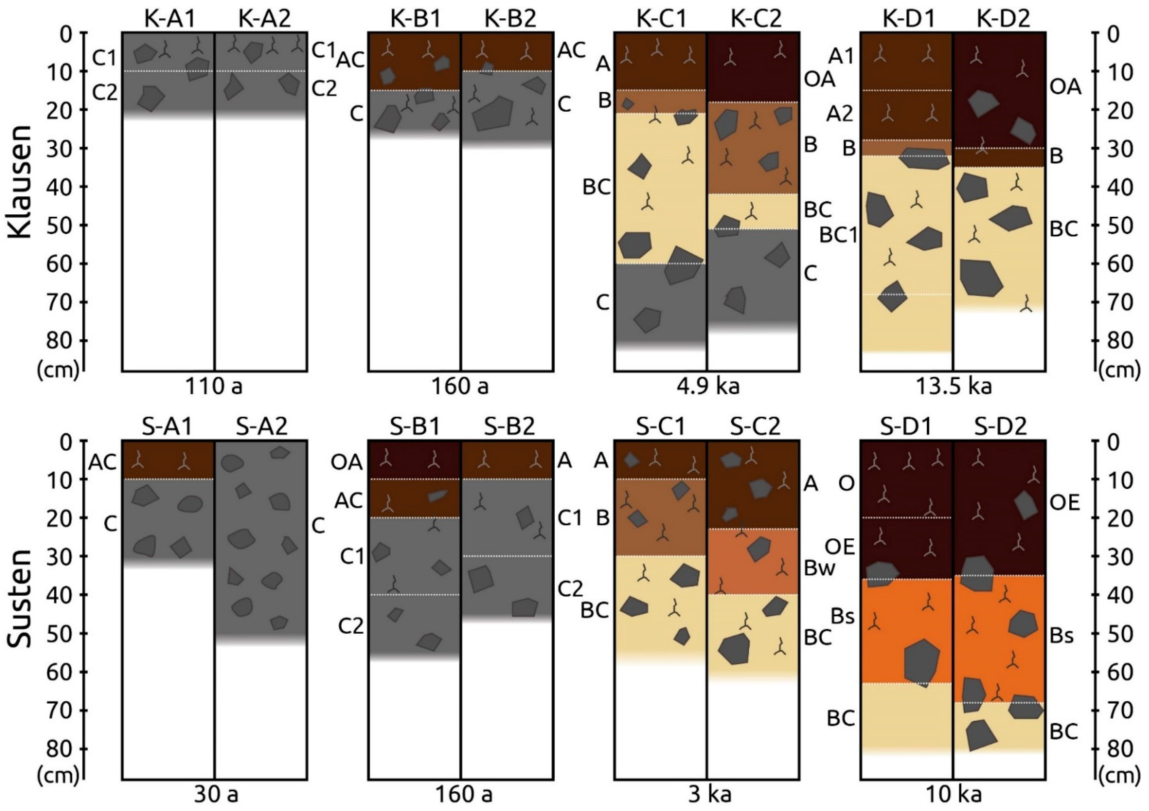
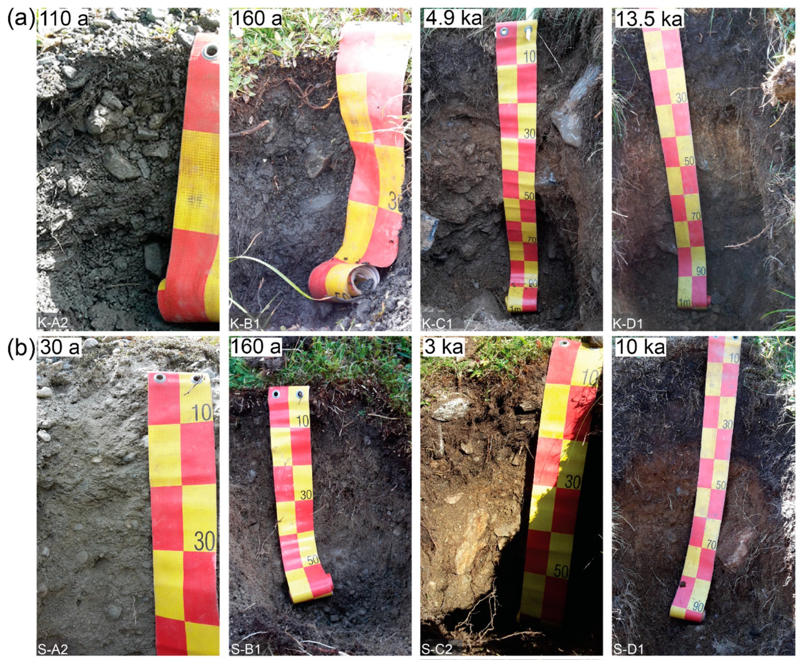
4.1. Profile Descriptions
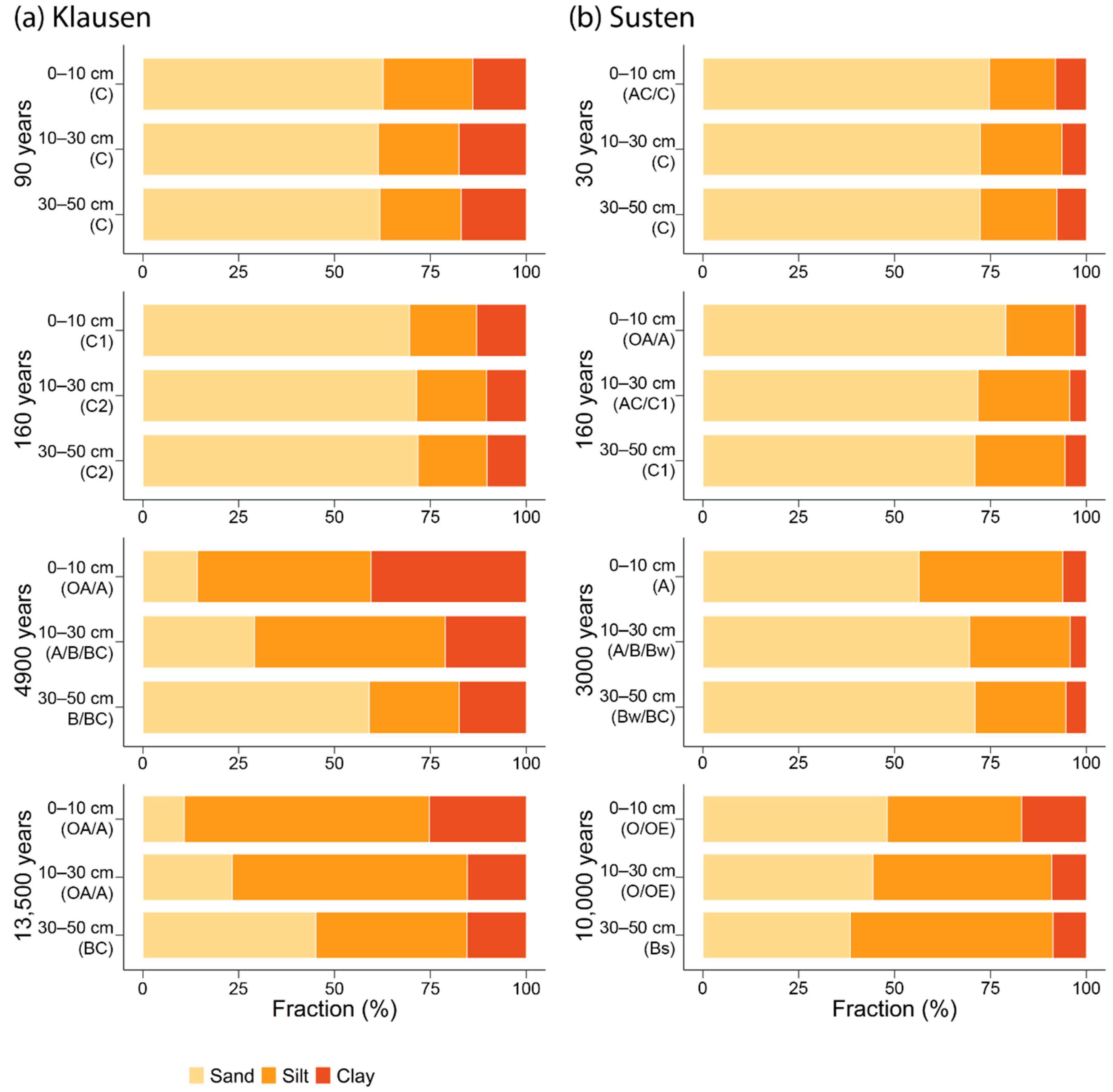
4.2. Soil Properties
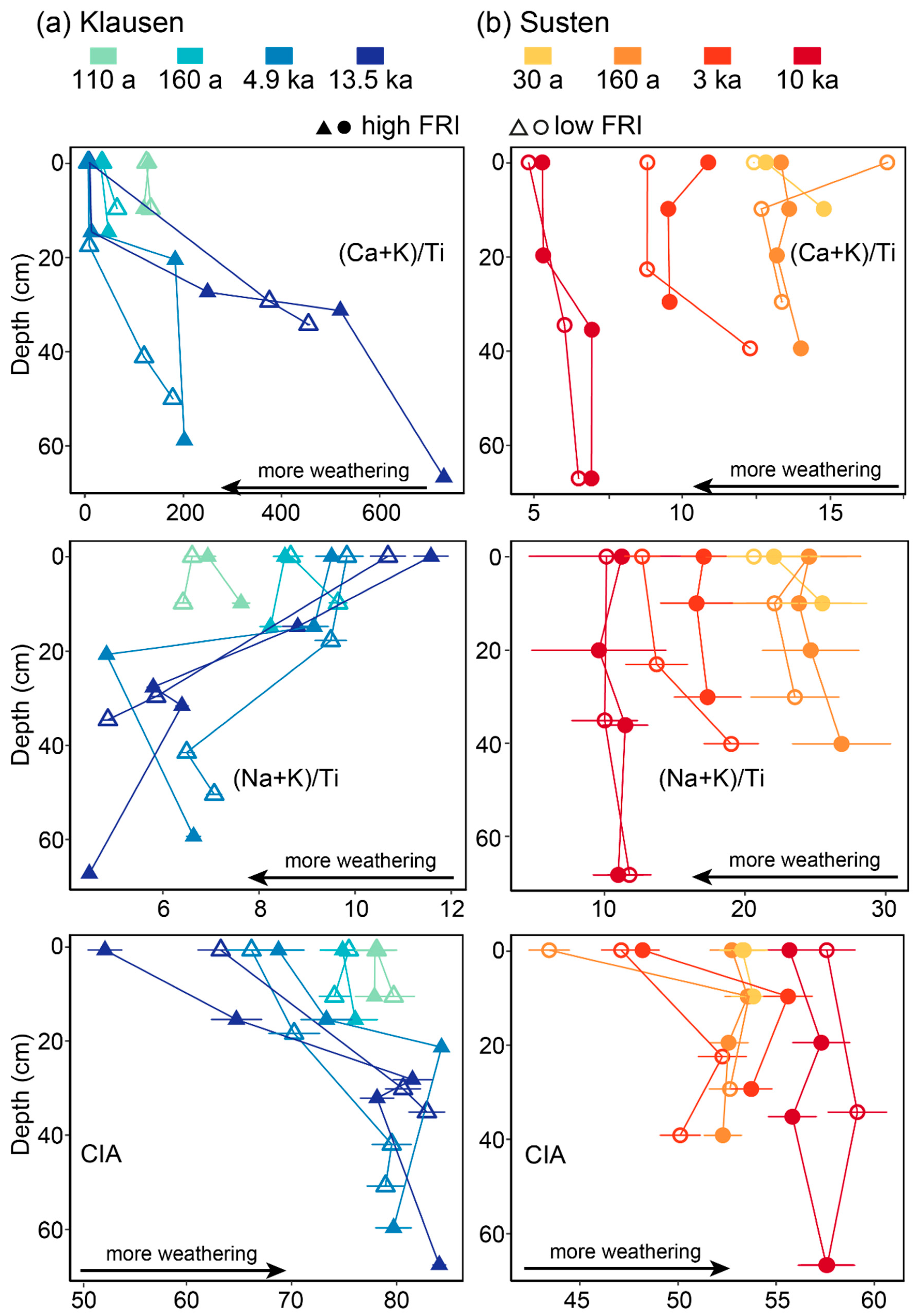
4.3. Weathering
4.3.1. Klausenpass
4.3.2. Sustenpass
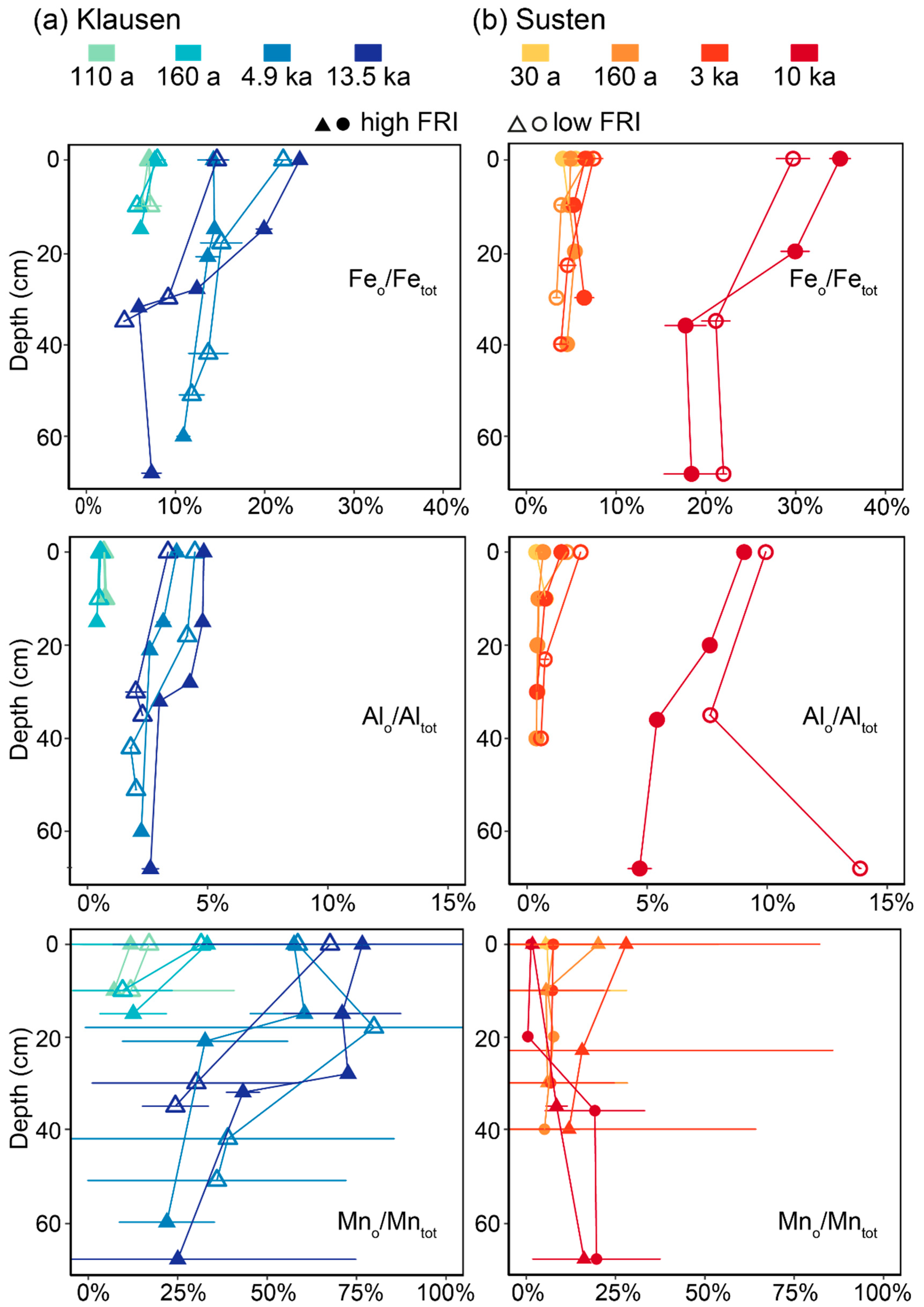
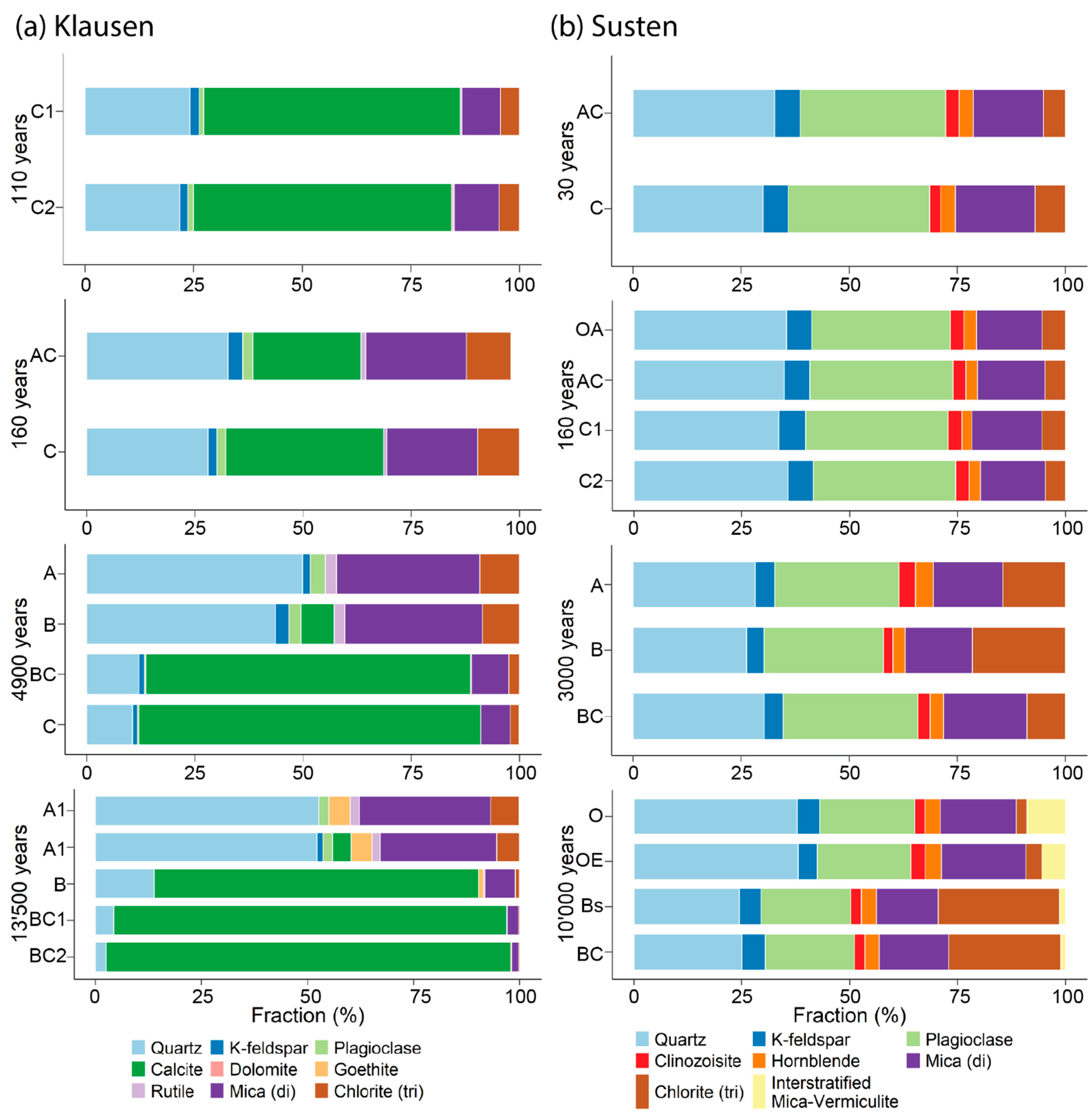
4.4. Mineralogy
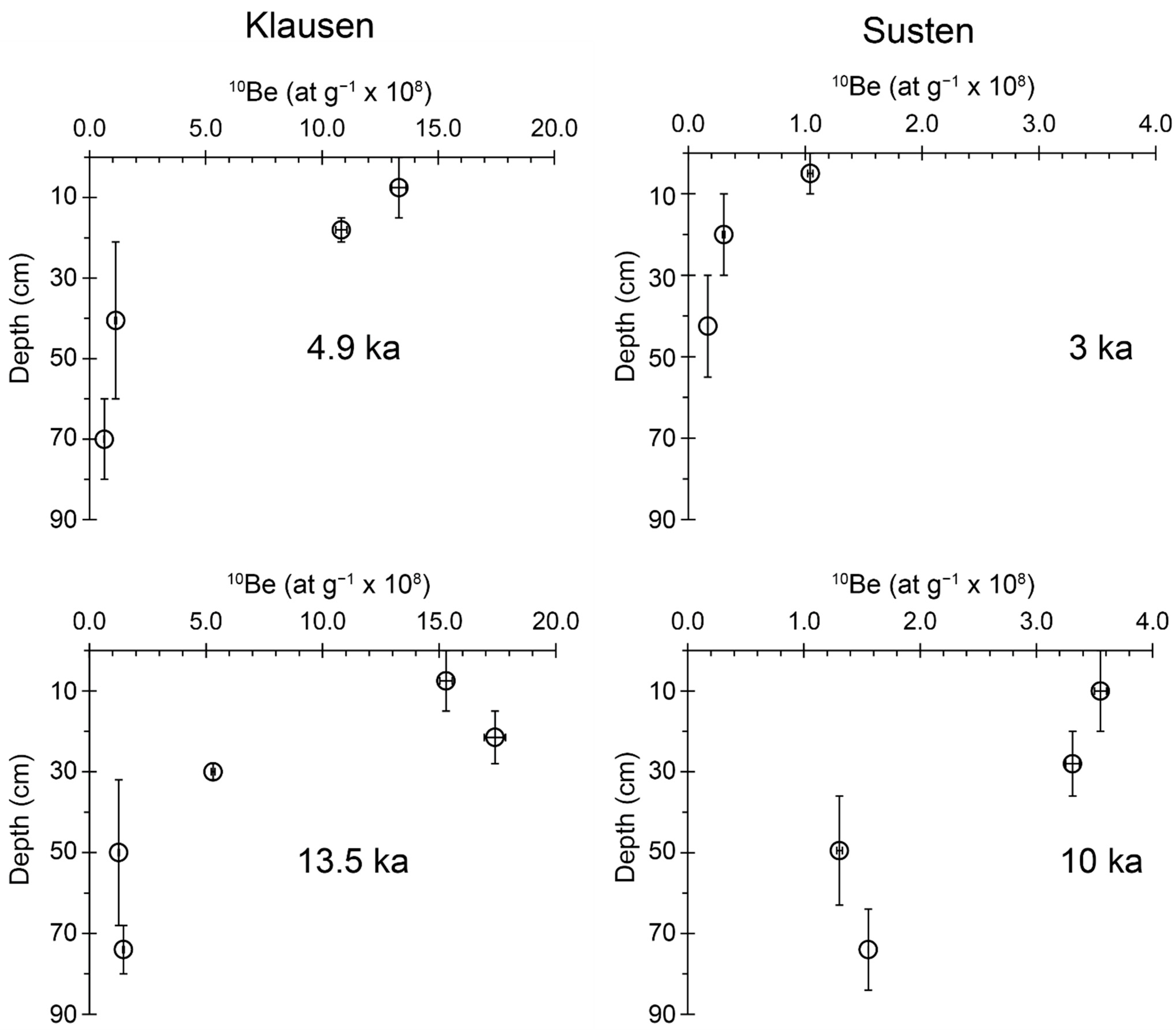
4.5. Meteoric 10Be Inventories and Erosion Rates
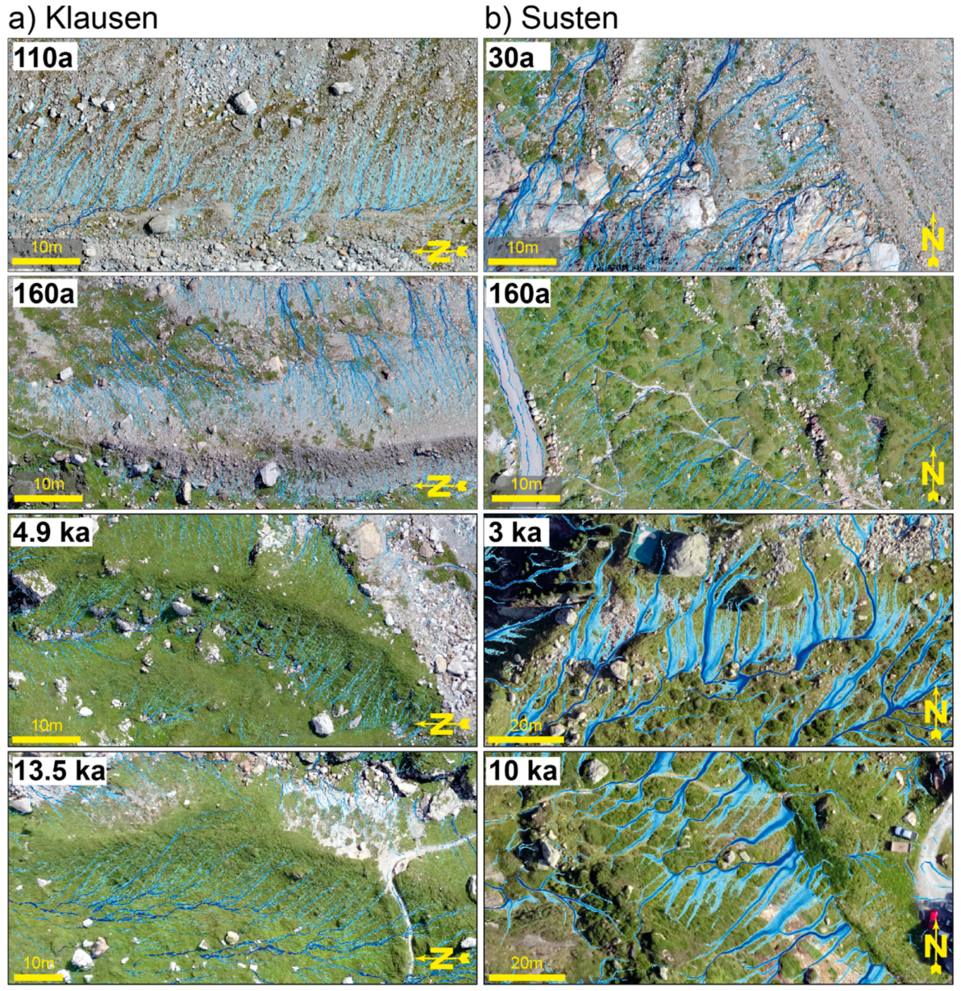
4.6. Flow Accumulation
5. Discussion
5.1. Soil Development in Calcareous Parent Material
5.2. Soil Development in Siliceous Parent Material
5.3. Soil Production vs. Erosion
5.4. Interaction with Vegetation and Hydrology

6. Conclusions
Author Contributions
Funding
Data Availability Statement
Acknowledgments
Conflicts of Interest
References
- Dokuchaev, V.V. Russkii Chernozem; Moscow, Russia, 1883. [Google Scholar]
- Jenny, H. Factors of Soil Formation: A System of Quantitative Pedology; McGraw-Hill: New York, NY, USA, 1941. [Google Scholar]
- Simonson, R.W. Outline of a Generalized Theory of Soil Genesis. Soil Sci. Soc. Am. J. 1959, 23, 152–156. [Google Scholar] [CrossRef]
- Johnson, D.L.; Watson-Stegner, D. Evolution Model of Pedogenesis. Soil Sci. 1987, 143, 349–366. [Google Scholar] [CrossRef]
- Egli, M.; Poulenard, J. Soils of Mountainous Landscapes. In International Encyclopedia of Geography: People, the Earth, Environment and Technology; Richardson, D., Castree, N., Goodchild, M.F., Kobayashi, A., Liu, W., Marston, R.A., Eds.; John Wiley & Sons, Ltd.: Oxford, UK, 2016; pp. 1–10. [Google Scholar]
- Sommer, M.; Gerke, H.H.; Deumlich, D. Modelling soil landscape genesis—A “time split” approach for hummocky agricultural landscapes. Geoderma 2008, 145, 480–493. [Google Scholar] [CrossRef]
- Dosseto, A.; Buss, H.; Suresh, P. The delicate balance between soil production and erosion, and its role on landscape evolution. Appl. Geochem. 2011, 26, S24–S27. [Google Scholar] [CrossRef] [Green Version]
- Heimsath, A.M.; Dietrich, W.E.; Nishiizumi, K.; Finkel, R.C. The soil production function and landscape equilibrium. Nature 1997, 388, 358–361. [Google Scholar] [CrossRef]
- Riebe, C.S.; Kirchner, J.; Finkel, R.C. Long-term rates of chemical weathering and physical erosion from cosmogenic nuclides and geochemical mass balance. Geochim. Cosmochim. Acta 2003, 67, 4411–4427. [Google Scholar] [CrossRef]
- von Blanckenburg, F.; Hewawasam, T.; Kubik, P.W. Cosmogenic nuclide evidence for low weathering and denudation in the wet, tropical highlands of Sri Lanka. J. Geophys. Res. Earth Surf. 2004, 109. [Google Scholar] [CrossRef]
- Cannone, N.; Diolaiuti, G.; Guglielmin, M.; Smiraglia, C. Accelerating Climate Change Impacts on Alpine Glacier Forefield Ecosystems in the European Alps. Ecol. Appl. 2008, 18, 637–648. [Google Scholar] [CrossRef] [Green Version]
- Delaney, I.; Bauder, A.; Huss, M.; Weidmann, Y. Proglacial erosion rates and processes in a glacierized catchment in the Swiss Alps. Earth Surf. Process. Landf. 2018, 43, 765–778. [Google Scholar] [CrossRef] [Green Version]
- Huggett, R. Soil chronosequences, soil development, and soil evolution: A critical review. CATENA 1998, 32, 155–172. [Google Scholar] [CrossRef]
- Sauer, D.; Schülli-Maurer, I.; Wagner, S.; Scarciglia, F.; Sperstad, R.; Svendgård-Stokke, S.; Sørensen, R.; Schellmann, G. Soil development over millennial timescales—A comparison of soil chronosequences of different climates and lithologies. IOP Conf. Ser. Earth Environ. Sci. 2015, 25, 12009. [Google Scholar] [CrossRef] [Green Version]
- White, A.F.; Blum, A.E.; Schulz, M.; Bullen, T.D.; Harden, J.W.; Peterson, M.L. Chemical weathering rates of a soil chronosequence on granitic alluvium: I. Quantification of mineralogical and surface area changes and calculation of primary silicate reaction rates. Geochim. Cosmochim. Acta 1996, 60, 2533–2550. [Google Scholar] [CrossRef]
- Bain, D.; Mellor, A.; Robertson-Rintoul, M.; Buckland, S. Variations in weathering processes and rates with time in a chronosequence of soils from Glen Feshie, Scotland. Geoderma 1993, 57, 275–293. [Google Scholar] [CrossRef]
- Taylor, A.; Blum, J.D. Relation between soil age and silicate weathering rates determined from the chemical evolution of a glacial chronosequence. Geology 1995, 23, 979–982. [Google Scholar] [CrossRef] [Green Version]
- Mavris, C.; Egli, M.; Plötze, M.; Blum, J.D.; Mirabella, A.; Giaccai, D.; Haeberli, W. Initial stages of weathering and soil formation in the Morteratsch proglacial area (Upper Engadine, Switzerland). Geoderma 2010, 155, 359–371. [Google Scholar] [CrossRef]
- Vilmundardóttir, O.K.; Gísladóttir, G.; Lal, R. Between ice and ocean; soil development along an age chronosequence formed by the retreating Breiðamerkurjökull glacier, SE-Iceland. Geoderma 2015, 259–260, 310–320. [Google Scholar] [CrossRef]
- D’Amico, M.E.; Freppaz, M.; Filippa, G.; Zanini, E. Vegetation influence on soil formation rate in a proglacial chronosequence (Lys Glacier, NW Italian Alps). CATENA 2014, 113, 122–137. [Google Scholar] [CrossRef]
- Righi, D. Clay Formation and Podzol Development from Postglacial Moraines in Switzerland. Clay Miner. 1999, 34, 319–332. [Google Scholar] [CrossRef]
- Bockheim, J.G. Solution and use of chronofunctions in studying soil development. Geoderma 1980, 24, 71–85. [Google Scholar] [CrossRef]
- Egli, M.; Fitze, P.; Mirabella, A. Weathering and evolution of soils formed on granitic, glacial deposits: Results from chronosequences of Swiss alpine environments. CATENA 2001, 45, 19–47. [Google Scholar] [CrossRef]
- Egli, M.; Fitze, P. Quantitative aspects of carbonate leaching of soils with differing ages and climates. CATENA 2001, 46, 35–62. [Google Scholar] [CrossRef]
- Egli, M.; Mirabella, A.; Fitze, P. Clay mineral formation in soils of two different chronosequences in the Swiss Alps. Geoderma 2001, 104, 145–175. [Google Scholar] [CrossRef]
- Föllmi, K.B.; Arn, K.; Hosein, R.; Adatte, T.; Steinmann, P. Biogeochemical weathering in sedimentary chronosequences of the Rhône and Oberaar Glaciers (Swiss Alps): Rates and mechanisms of biotite weathering. Geoderma 2009, 151, 270–281. [Google Scholar] [CrossRef]
- Mavris, C.; Plötze, M.; Mirabella, A.; Giaccai, D.; Valboa, G.; Egli, M. Clay mineral evolution along a soil chronosequence in an Alpine proglacial area. Geoderma 2011, 165, 106–117. [Google Scholar] [CrossRef] [Green Version]
- Birkeland, P.W. Soils and Geomorphology; Oxford University Press Inc.: New York, NY, USA; Oxford, UK, 1984. [Google Scholar]
- Haselberger, S.; Ohler, L.-M.; Junker, R.R.; Otto, J.-C.; Glade, T.; Kraushaar, S. Quantification of biogeomorphic interactions between small-scale sediment transport and primary vegetation succession on proglacial slopes of the Gepatschferner, Austria. Earth Surf. Process. Landf. 2021, 46, 1941–1952. [Google Scholar] [CrossRef]
- Eichel, J.; Corenblit, D.; Dikau, R. Conditions for feedbacks between geomorphic and vegetation dynamics on lateral moraine slopes: A biogeomorphic feedback window. Earth Surf. Process. Landf. 2016, 41, 406–419. [Google Scholar] [CrossRef]
- Dümig, A.; Smittenberg, R.; Kögel-Knabner, I. Concurrent evolution of organic and mineral components during initial soil development after retreat of the Damma glacier, Switzerland. Geoderma 2011, 163, 83–94. [Google Scholar] [CrossRef]
- Burga, C.A. Vegetation development on the glacier forefield Morteratsch (Switzerland). Appl. Veg. Sci. 1999, 2, 17–24. [Google Scholar] [CrossRef]
- Hudek, C.; Stanchi, S.; D’Amico, M.; Freppaz, M. Quantifying the contribution of the root system of alpine vegetation in the soil aggregate stability of moraine. Int. Soil Water Conserv. Res. 2017, 5, 36–42. [Google Scholar] [CrossRef]
- Kumar, R.; Pandey, S.; Pandey, A. Plant roots and carbon sequestration. Curr. Sci. 2006, 91, 885–890. [Google Scholar]
- Tresder, K.K.; Morris, S.J.; Allen, M.F. The Contribution of Root Exudates, Symbionts, and Detritus to Carbon Sequestration in the Soil. In Roots and Soil Management: Interactions between Roots and the Soil; Zobel, R.W., Wright, S.F., Eds.; Agronomy No. 48; American Society of Agronomy: Madison, WI, USA, 2005; pp. 145–162. [Google Scholar]
- Khedim, N.; Cécillon, L.; Poulenard, J.; Barré, P.; Baudin, F.; Marta, S.; Rabatel, A.; Dentant, C.; Cauvy-Fraunié, S.; Anthelme, F.; et al. Topsoil organic matter build-up in glacier forelands around the world. Glob. Chang. Biol. 2021, 27, 1662–1677. [Google Scholar] [CrossRef] [PubMed]
- Montagnani, L.; Badraghi, A.; Speak, A.F.; Wellstein, C.; Borruso, L.; Zerbe, S.; Zanotelli, D. Evidence for a non-linear carbon accumulation pattern along an Alpine glacier retreat chronosequence in Northern Italy. PeerJ 2019, 7, e7703. [Google Scholar] [CrossRef] [PubMed]
- Zhang, B.; Yang, Y.-S.; Zepp, H. Effect of vegetation restoration on soil and water erosion and nutrient losses of a severely eroded clayey Plinthudult in southeastern China. CATENA 2004, 57, 77–90. [Google Scholar] [CrossRef]
- Burga, C.A.; Krüsi, B.; Egli, M.; Wernli, M.; Elsener, S.; Ziefle, M.; Fischer, T.; Mavris, C. Plant succession and soil development on the foreland of the Morteratsch glacier (Pontresina, Switzerland): Straight forward or chaotic? Flora Morphol. Distrib. Funct. Ecol. Plants 2010, 205, 561–576. [Google Scholar] [CrossRef] [Green Version]
- Hinsinger, P. Plant-induced changes in soil processes and properties. In Soil Conditions and Plant Growth; Gregory, P.J., Nortcliff, S., Eds.; Wiley-Blackwell: Chichester, West Sussex, UK; Ames, IA, USA, 2013; pp. 323–365. [Google Scholar]
- Walczak, R.; Rovdan, E.; Witkowska-Walczak, B. Water retention characteristics of peat and sand mixtures. Int. Agrophys. 2002, 16, 161–165. [Google Scholar]
- Yang, F.; Zhang, G.-L.; Yang, J.-L.; Li, D.-C.; Zhao, Y.-G.; Liu, F.; Yang, R.-M.; Yang, F. Organic matter controls of soil water retention in an alpine grassland and its significance for hydrological processes. J. Hydrol. 2014, 519, 3086–3093. [Google Scholar] [CrossRef]
- Faucon, M.-P.; Houben, D.; Lambers, H. Plant Functional Traits: Soil and Ecosystem Services. Trends Plant Sci. 2017, 22, 385–394. [Google Scholar] [CrossRef]
- Villéger, S.; Mason, N.W.H.; Mouillot, D. New Multidimensional Functional Diversity Indices for a Multifaceted Framework in Functional Ecology. Ecology 2008, 89, 2290–2301. [Google Scholar] [CrossRef] [Green Version]
- Mason, N.W.H.; de Bello, F. Functional diversity: A tool for answering challenging ecological questions. J. Veg. Sci. 2013, 24, 777–780. [Google Scholar] [CrossRef]
- Willenbring, J.K.; von Blanckenburg, F. Meteoric cosmogenic Beryllium-10 adsorbed to river sediment and soil: Applications for Earth-surface dynamics. Earth-Sci. Rev. 2010, 98, 105–122. [Google Scholar] [CrossRef] [Green Version]
- Lal, D. New methods for studies of soil dynamics utilizing cosmic ray produced radionuclides. In Sustaining the Global Farm. 10th International Soil Conservation Organization Meeting; Stott, D.E., Mohtar, R.H., Steinhardt, G.C., Eds.; Purdue University and USDA-ARS National Soil Erosion Research Laboratory: Purdue, IN, USA, 2001; pp. 1044–1052. [Google Scholar]
- Heikkilä, U.; Beer, J.; Feichter, J. Meridional transport and deposition of atmospheric 10Be. Atmos. Chem. Phys. 2009, 9, 515–527. [Google Scholar] [CrossRef] [Green Version]
- Foster, M.; Anderson, R.S.; Wyshnytzky, C.E.; Ouimet, W.B.; Dethier, D.P. Hillslope loweing rates and mobile-regolith residence times from in situ and meteoric 10Be analysis, Boulder Creek Critical Zone Observatory, Colorado. GSA Bull. 2015, 127, 862–878. [Google Scholar] [CrossRef]
- Schoonejans, J.; Vanacker, V.; Opfergelt, S.; Christl, M. Long-term soil erosion derived from in-situ 10Be and inventories of meteoric 10Be in deeply weathered soils in southern Brazil. Chem. Geol. 2017, 466, 380–388. [Google Scholar] [CrossRef]
- Maier, F.; van Meerveld, I.; Greinwald, K.; Gebauer, T.; Lustenberger, F.; Hartmann, A.; Musso, A. Effects of soil and vegetation development on surface hydrological properties of moraines in the Swiss Alps. CATENA 2020, 187, 104353. [Google Scholar] [CrossRef]
- Helming, K.; Römkens, M.J.M.; Prasad, S.N. Surface Roughness Related Processes of Runoff and Soil Loss: A Flume Study. Soil Sci. Soc. Am. J. 1998, 62, 243–250. [Google Scholar] [CrossRef]
- Musso, A.; Ketterer, M.E.; Greinwald, K.; Geitner, C.; Egli, M. Rapid decrease of soil erosion rates with soil formation and vegetation development in periglacial areas. Earth Surf. Process. Landf. 2020, 45, 2824–2839. [Google Scholar] [CrossRef]
- Greinwald, K.; Dieckmann, L.A.; Schipplick, C.; Hartmann, A.; Scherer-Lorenzen, M.; Gebauer, T. Vertical root distribution and biomass allocation along proglacial chronosequences in Central Switzerland. Arct. Antarct. Alp. Res. 2021, 53, 20–34. [Google Scholar] [CrossRef]
- Hartmann, A.; Weiler, M.; Blume, T. The impact of landscape evolution on soil physics: Evolution of soil physical and hydraulic properties along two chronosequences of proglacial moraines. Earth Syst. Sci. Data 2020, 12, 3189–3204. [Google Scholar] [CrossRef]
- Maier, F.; van Meerveld, I. Long-Term Changes in Runoff Generation Mechanisms for Two Proglacial Areas in the Swiss Alps I: Overland Flow. Water Resour. Res. 2021, 57, e2021WR030221. [Google Scholar] [CrossRef]
- Bundesamt für Landestopographie (Swisstopo). Geologische Karte der Schweiz. 2008. Available online: https://s.geo.admin.ch/8f6671cce7 (accessed on 1 December 2021).
- Meteoswiss. Climate Normals Temperature 1961–1990. 2019. Available online: https://s.geo.admin.ch/93c9144885 (accessed on 20 October 2021).
- Meteoswiss. Climate Normals Precipitation 1961–1990. 2019. Available online: https://s.geo.admin.ch/93c91528d3 (accessed on 20 October 2021).
- Bundesamt für Landestopographie (Swisstopo). Siegfriedkarte: TA50, Blatt 403. 1899. Available online: https://s.geo.admin.ch/8f679fc9f6 (accessed on 1 December 2021).
- Ivy-Ochs, S.; Kerschner, H.; Maisch, M.; Christl, M.; Kubik, P.W.; Schlüchter, C. Latest Pleistocene and Holocene glacier variations in the European Alps. Quat. Sci. Rev. 2009, 28, 2137–2149. [Google Scholar] [CrossRef]
- Musso, A.; Lamorski, K.; Sławiński, C.; Geitner, C.; Hunt, A.; Greinwald, K.; Egli, M. Evolution of soil pores and their characteristics in a siliceous and calcareous proglacial area. CATENA 2019, 182, 104154. [Google Scholar] [CrossRef]
- Bundesamt für Landestopographie (Swisstopo). Aerial Image. 1988. Available online: https://s.geo.admin.ch/8804d2594d (accessed on 15 December 2019).
- Bundesamt für Landestopographie (Swisstopo). Aerial Image. 1992. Available online: https://s.geo.admin.ch/8804d210f5 (accessed on 15 December 2019).
- Bundesamt für Landestopographie (Swisstopo). Aerial Image. 1993. Available online: https://s.geo.admin.ch/8804cdd7ca (accessed on 15 December 2019).
- King, L. Studien zur postglazialen Gletscher- und Vegetationsgeschichte des Sustenpassgebietes, 2nd ed.; Helbing und Lichtenhahn: Basel, Switzerland, 1974. [Google Scholar]
- Heikkinen, O.; Fogelberg, P. Bodenentwicklung im Hochgebirge: Ein Beispiel vom Vorfeld des Steingletschers in der Schweiz. Geogr. Helv. 1980, 35, 107–112. [Google Scholar] [CrossRef] [Green Version]
- Schimmelpfennig, I.; Schaefer, J.M.; Akçar, N.; Koffman, T.; Ivy-Ochs, S.; Schwartz, R.; Finkel, R.C.; Zimmerman, S.; Schlüchter, C. A chronology of Holocene and Little Ice Age glacier culminations of the Steingletscher, Central Alps, Switzerland, based on high-sensitivity beryllium-10 moraine dating. Earth Planet. Sci. Lett. 2014, 393, 220–230. [Google Scholar] [CrossRef] [Green Version]
- FAO. World reference base for soil resources 2014. In International Soil Classification System for Naming Soils and Creating Legends for Soil Maps; World Soil Resources Reports 106; FAO: Rome, Italy, 2014. [Google Scholar]
- Tilman, D. Functional diversity. In Encyclopedia of Biodiversity; Levin, S.A., Ed.; Academic Press: San Diego, CA, USA, 2001; pp. 109–120. [Google Scholar]
- Lauber, K.; Wagner, G.; Gygax, A. (Eds.) Flora Helvetica: Illustrierte Flora der Schweiz: Mit Artbeschreibungen und Verbreitungskarten von 3200 wild Wachsenden Farn- und Blütenpflanzen, Einschliesslich Wichtiger Kulturpflanzen; Sechste, Vollständig Überarbeitete Auflage; Haupt Verlag: Bern, Switzerland, 2018. [Google Scholar]
- Heiri, O.; Lotter, A.F.; Lemcke, G. Loss on ignition as a method for estimating organic and carbonate content in sediments: Reproducibility and comparability of results. J. Paleolimnol. 2001, 25, 101–110. [Google Scholar] [CrossRef]
- Dorn, R. Cation-ratio dating: A new rock varnish age-de-termination technique. Quat. Res. 1983, 20, 49–73. [Google Scholar] [CrossRef]
- Stiles, C.A.; Mora, C.I.; Driese, S.G. Pedogenic processes and domain boundaries in a Vertisol climosequence: Evidence from titanium and zirconium distribution and morphology. Geoderma 2003, 116, 279–299. [Google Scholar] [CrossRef]
- Nesbitt, H.W.; Young, G.M. Early Proterozoic climates and plate motions inferred from major element chemistry of lutites. Nature 1982, 299, 715–717. [Google Scholar] [CrossRef]
- McKeague, J.A.; Brydon, J.E.; Miles, N.M. Differentiation of Forms of Extractable Iron and Aluminum in Soils. Soil Sci. Soc. Am. J. 1971, 35, 33–38. [Google Scholar] [CrossRef]
- Zhang, G.; Germaine, J.T.; Martin, T.; Whittle, A.J. A simple sample-mounting method for random powder X-ray diffraction. Clays Clay Miner. 2003, 51, 218–225. [Google Scholar] [CrossRef]
- Döbelin, N.; Kleeberg, R. Profex: A graphical user interface for the Rietveld refinement program BGMN. J. Appl. Crystallogr. 2015, 48, 1573–1580. [Google Scholar] [CrossRef] [Green Version]
- von Blanckenburg, F.; Belshaw, N.; O’Nions, R. Separation of 9Be and cosmogenic 10Be from environmental materials and SIMS isotope dilution analysis. Chem. Geol. 1996, 129, 93–99. [Google Scholar] [CrossRef]
- Christl, M.; Vockenhuber, C.; Kubik, P.; Wacker, L.; Lachner, J.; Alfimov, V.; Synal, H.-A. The ETH Zurich AMS facilities: Performance parameters and reference materials. Nucl. Instrum. Methods Phys. Res. Sect. B Beam Interact. Mater. At. 2013, 294, 29–38. [Google Scholar] [CrossRef]
- Nishiizumi, K.; Imamura, M.; Caffee, M.W.; Southon, J.R.; Finkel, R.C.; McAninch, J. Absolute calibration of 10Be AMS standards. Nucl. Instrum. Methods Phys. Res. Sect. B Beam Interact. Mater. At. 2007, 258, 403–413. [Google Scholar] [CrossRef]
- Chadwick, O.A.; Brimhall, G.H.; Hendricks, D.M. From a black to a gray box—A mass balance interpretation of pedogenesis. Geomorphology 1990, 3, 369–390. [Google Scholar] [CrossRef]
- Egli, M.; Fitze, P. Formulation of pedologic mass balance based on immobile elements: A revision. Soil Sci. 2000, 165, 437–443. [Google Scholar] [CrossRef]
- Maejima, Y.; Matsuzaki, H.; Higashi, T. Application of cosmogenic 10Be to dating soils on the raised coral reef terraces of Kikai Island, southwest Japan. Geoderma 2005, 126, 389–399. [Google Scholar] [CrossRef]
- Tsai, C.; Chen, Z.; Kao, C.; Ottner, F.; Kao, S.; Zehetner, F. Pedogenic development of volcanic ash soils along a climosequence in Northern Taiwan. Geoderma 2010, 156, 48–59. [Google Scholar] [CrossRef]
- Egli, M.; Brandová, D.; Böhlert, R.; Favilli, F.; Kubik, P.W. 10Be inventories in Alpine soils and their potential for dating land surfaces. Geomorphology 2010, 119, 62–73. [Google Scholar] [CrossRef] [Green Version]
- Graly, J.A.; Reusser, L.J.; Bierman, P.R. Short and long-term delivery rates of meteoric 10Be to terrestrial soils. Earth Planet. Sci. Lett. 2011, 302, 329–336. [Google Scholar] [CrossRef]
- Deng, K.; Wittmann, H.; von Blanckenburg, F. The depositional flux of meteoric cosmogenic 10Be from modeling and observation. Earth Planet. Sci. Lett. 2020, 550, 116530. [Google Scholar] [CrossRef]
- Phillips, J.D.; Marion, D.A.; Luckow, K.; Adams, K.R. Nonequilibrium Regolith Thickness in the Ouachita Mountains. J. Geol. 2005, 113, 325–340. [Google Scholar] [CrossRef]
- Johnson, D.; Domier, J.; Johnson, D.N. Animating the biodynamics of soil thickness using process vector analysis: A dynamic denudation approach to soil formation. Geomorphology 2005, 67, 23–46. [Google Scholar] [CrossRef]
- Egli, M.; Dahms, D.; Norton, K. Soil formation rates on silicate parent material in alpine environments: Different approaches–different results? Geoderma 2014, 213, 320–333. [Google Scholar] [CrossRef] [Green Version]
- Lustenberger, F. Event-Based Surface Hydrological Connectivity and Sediment Transport on Young Moraines. Master’s Thesis, University of Zurich, Zurich, Switzerland, 2019. [Google Scholar]
- Tarboton, D.G. A new method for the determination of flow directions and upslope areas in grid digital elevation models. Water Resour. Res. 1997, 33, 309–319. [Google Scholar] [CrossRef] [Green Version]
- Joint Committee for Guides in Metrology. JCGM 100:2008: Guide to the Expression of Uncertainty in Measurement (JCGM); BIPM: Sevres, France, 2008. [Google Scholar]
- Martignier, L.; Verrecchia, E.P. Weathering processes in superficial deposits (regolith) and their influence on pedogenesis: A case study in the Swiss Jura Mountains. Geomorphology 2013, 189, 26–40. [Google Scholar] [CrossRef]
- Egli, M.; Merkli, C.; Sartori, G.; Mirabella, A.; Plötze, M. Weathering, mineralogical evolution and soil organic matter along a Holocene soil toposequence developed on carbonate-rich materials. Geomorphology 2008, 97, 675–696. [Google Scholar] [CrossRef]
- Allen, C.; Darmody, R.; Thorn, C.; Dixon, J.; Schlyter, P. Clay mineralogy, chemical weathering and landscape evolution in Arctic–Alpine Sweden. Geoderma 2001, 99, 277–294. [Google Scholar] [CrossRef]
- Egli, M.; Sartori, G.; Mirabella, A.; Giaccai, D. The effects of exposure and climate on the weathering of late Pleistocene and Holocene Alpine soils. Geomorphology 2010, 114, 466–482. [Google Scholar] [CrossRef] [Green Version]
- Böhlert, R.; Mirabella, A.; Plötze, M.; Egli, M. Landscape evolution in Val Mulix, eastern Swiss Alps—Soil chemical and mineralogical analyses as age proxies. Catena 2011, 87, 313–325. [Google Scholar] [CrossRef] [Green Version]
- Mahaney, W.; Kalm, V.; Kapran, B.; Milner, M.; Hancock, R. A soil chronosequence in Late Glacial and Neoglacial moraines, Humboldt Glacier, northwestern Venezuelan Andes. Geomorphology 2009, 109, 236–245. [Google Scholar] [CrossRef]
- Earl-Goulet, J.R.; Mahaney, W.C.; Sanmugadas, K.; Kalm, V.; Hancock, R.G. Middle-Holocene timberline fuctuation: Influence on the genesis of Podzols (Spodosols), Norra Storfjället Massif, northern Sweden. Holocene 1998, 8, 705–718. [Google Scholar] [CrossRef]
- Eger, A.; Almond, P.C.; Condron, L.M. Pedogenesis, soil mass balance, phosphorus dynamics and vegetation communities across a Holocene soil chronosequence in a super-humid climate, South Westland, New Zealand. Geoderma 2011, 163, 185–196. [Google Scholar] [CrossRef]
- Dahlgren, R.; Boettinger, J.; Huntington, G.; Amundson, R. Soil development along an elevational transect in the western Sierra Nevada, California. Geoderma 1997, 78, 207–236. [Google Scholar] [CrossRef]
- Hartmann, A.; Semenova, E.; Weiler, M.; Blume, T. Field observations of soil hydrological flow path evolution over 10 millennia. Hydrol. Earth Syst. Sci. 2020, 24, 3271–3288. [Google Scholar] [CrossRef]
- Chen, P.; Yi, P.; Czymzik, M.; Aldahan, A.; Ljung, K.; Yu, Z.; Hou, X.; Zheng, M.; Chen, X.; Possnert, G. Relationship between precipitation and 10Be and impacts on soil dynamics. CATENA 2020, 195, 104748. [Google Scholar] [CrossRef]
- Zollinger, B.; Alewell, C.; Kneisel, C.; Meusburger, K.; Brandová, D.; Kubik, P.; Schaller, M.; Ketterer, M.; Egli, M. The effect of permafrost on time-split soil erosion using radionuclides (137Cs, 239 + 240Pu, meteoric 10Be) and stable isotopes (δ 13C) in the eastern Swiss Alps. J. Soils Sediments 2015, 15, 1400–1419. [Google Scholar] [CrossRef]
- Norton, K.P.; von Blanckenburg, F.; Kubik, P.W. Cosmogenic nuclide-derived rates of diffusive and episodic erosion in the glacially sculpted upper Rhone Valley, Swiss Alps. Earth Surf. Process. Landf. 2010, 35, 651–662. [Google Scholar] [CrossRef] [Green Version]
- Larsen, I.J.; Almond, P.C.; Eger, A.; Stone, J.O.; Montgomery, D.R.; Malcolm, B. Rapid Soil Production and Weathering in the Southern Alps, New Zealand. Science 2014, 343, 637–640. [Google Scholar] [CrossRef] [Green Version]
- Renard, K.; Foster, G.R.; Weesies, G.A.; McCool, D.K.; Yoder, D.C. (Eds.) Predicting Soil Erosion by Water: A Guide to Conservation Planning with the Revised Universal Soil Loss Equation (RUSLE); USDA, Agricultural Research Service: Washington, DC, USA, 1997.
- Saedi, T.; Shorafa, M.; Gorji, M.; Moghadam, B.K. Indirect and direct effects of soil properties on soil splash erosion rate in calcareous soils of the central Zagross, Iran: A laboratory study. Geoderma 2016, 271, 1–9. [Google Scholar] [CrossRef]
- Pintaldi, E.; D’Amico, M.E.; Stanchi, S.; Catoni, M.; Freppaz, M.; Bonifacio, E. Humus forms affect soil susceptibility to water erosion in the Western Italian Alps. Appl. Soil Ecol. 2018, 123, 478–483. [Google Scholar] [CrossRef]
- Stanchi, S.; Falsone, G.; Bonifacio, E. Soil aggregation, erodibility, and erosion rates in mountain soils (NW Alps, Italy). Solid Earth 2015, 6, 403–414. [Google Scholar] [CrossRef] [Green Version]
- Darboux, F.; Huang, C. Does Soil Surface Roughness Increase or Decrease Water and Particle Transfers? Soil Sci. Soc. Am. J. 2005, 69, 748–756. [Google Scholar] [CrossRef] [Green Version]
- Luo, J.; Zheng, Z.; Li, T.; He, S. Assessing the impacts of microtopography on soil erosion under simulated rainfall, using a multifractal approach. Hydrol. Process. 2018, 32, 2543–2556. [Google Scholar] [CrossRef]
- Luo, J.; Zheng, Z.; Li, T.; He, S. Spatial variation of microtopography and its effect on temporal evolution of soil erosion during different erosive stages. CATENA 2020, 190, 104515. [Google Scholar] [CrossRef]
- Luo, J.; Zheng, Z.; Li, T.; He, S.; Zhang, X.; Huang, H.; Wang, Y. Quantifying the contributions of soil surface microtopography and sediment concentration to rill erosion. Sci. Total Environ. 2021, 752, 141886. [Google Scholar] [CrossRef] [PubMed]
- Alewell, C.; Egli, M.; Meusburger, K. An attempt to estimate tolerable soil erosion rates by matching soil formation with denudation in Alpine grasslands. J. Soils Sediments 2015, 15, 1383–1399. [Google Scholar] [CrossRef] [Green Version]
- Riebe, C.S.; Kirchner, J.W.; Granger, D.E.; Finkel, R.C. Strong tectonic and weak climatic control of long-term chemical weathering rates. Geology 2001, 29, 511. [Google Scholar] [CrossRef]
- Small, E.E.; Anderson, R.S.; Hancock, G.S. Estimates of the rate of regolith production using and from an alpine hillslope. Geomorphology 1999, 27, 131–150. [Google Scholar] [CrossRef]
- Dixon, J.L.; von Blanckenburg, F. Soils as pacemakers and limiters of global silicate weathering. Comptes Rendus Geosci. 2012, 344, 597–609. [Google Scholar] [CrossRef] [Green Version]
- Körner, C. Alpine plant life. In Functional Plant Ecology of High Mountain Ecosystems, 2nd ed.; Körner, C., Ed.; Springer: Heidelberg, Germany; New York, NY, USA, 2003. [Google Scholar]
- Saxton, K.E.; Rawls, W.J.; Romberger, J.S.; Papendick, R.I. Estimating generalized soil-water characteristics from texture. Soil Sci. Soc. Am. J. 1986, 50, 1031–1036. [Google Scholar] [CrossRef]
- Thorarinsdottir, E.F.; Arnalds, O. Wind erosion of volcanic materials in the Hekla area, South Iceland. Aeolian Res. 2012, 4, 39–50. [Google Scholar] [CrossRef]
- Dontsova, K.; Balogh-Brunstad, Z.; Chorover, J. Plants as drivers of rock weathering. In Biogeochemical Cycles: Ecological Drivers and Environmental Impact; Dontsova, K., Balogh-Brunstad, Z., Le Roux, G., Eds.; Wiley & Sons Inc.: Hoboken, NJ, USA; Americal Geophysical Union: Washington, DC, USA, 2020; pp. 33–58. [Google Scholar]
- Gild, C.; Geitner, C.; Sanders, D. Discovery of a landscape-wide drape of late-glacial aeolian silt in the western Northern Calcareous Alps (Austria): First results and implications. Geomorphology 2018, 301, 39–52. [Google Scholar] [CrossRef]
- R Core Team. R: A Language and Environment for Statistical Computing; R Foundation for Statistical Computing: Vienna, Austria, 2020. [Google Scholar]
- Egli, M.; Lessovaia, S.N.; Chistyakov, K.; Inozemzev, S.; Polekhovsky, Y.; Ganyushkin, D. Microclimate affects soil chemical and mineralogical properties of cold alpine soils of the Altai Mountains (Russia). J. Soils Sediments 2015, 15, 1420–1436. [Google Scholar] [CrossRef]
- Holtmeier, F.-K.; Broll, G. The Influence of Tree Islands and Microtopography on Pedoecological Conditions in the Forest-Alpine Tundra Ecotone on Niwot Ridge, Colorado Front Range, U.S.A. Artic Antarct. Alp. Res. 1992, 24, 216. [Google Scholar] [CrossRef]
- Lohse, K.A.; Dietrich, W.E. Contrasting effects of soil development on hydrological properties and flow paths. Water Resour. Res. 2005, 41, 1–17. [Google Scholar] [CrossRef]
- Wondzell, S.M.; Cornelius, J.M.; Cunningham, G.L. Vegetation patterns, microtopography, and soils on a Chihuahuan desert playa. J. Veg. Sci. 1990, 1, 403–410. [Google Scholar] [CrossRef]
- McGrath, G.S.; Paik, K.; Hinz, C. Microtopography alters self-organized vegetation patterns in water-limited ecosystems. J. Geophys. Res. Biogeosci. 2012, 117, 1–19. [Google Scholar] [CrossRef] [Green Version]


| Profile | Horizon | Depth | Na2O | MgO | Al2O3 | SiO2 | P2O5 | SO3 | K2O | CaCO3 | CaO | TiO2 | MnO | Fe2O3 | ZrO2 |
|---|---|---|---|---|---|---|---|---|---|---|---|---|---|---|---|
| cm | g/kg | g/kg | g/kg | g/kg | g/kg | g/kg | g/kg | g/kg | g/kg | g/kg | g/kg | g/kg | g/kg | ||
| Klausenpass (Griess Glacier) | |||||||||||||||
| 110 years | |||||||||||||||
| K-A1 | C1 | 0–10 | 3.23 ± 0.08 | 33.6 ± 0.44 | 54.09 ± 0.18 | 289.58 ± 0.42 | 1.76 ± 0.01 | 0.8 ± 0.01 | 9.23 ± 0.02 | 555.49 ± 0.24 | 0 ± 0.14 | 3.46 ± 0.01 | 0.35 ± 0 | 30.75 ± 0.03 | 0.16 ± 0 |
| C2 | 10–20+ | 3.87 ± 0.09 | 34.73 ± 0.43 | 63.43 ± 0.22 | 283.27 ± 0.41 | 1.78 ± 0.01 | 0.74 ± 0.01 | 10.75 ± 0.02 | 545.3 ± 0.24 | 0 ± 0.13 | 3.7 ± 0.01 | 0.33 ± 0 | 32.14 ± 0.03 | 0.13 ± 0 | |
| K-A2 | C1 | 0–10 | 3.19 ± 0.08 | 32.61 ± 0.43 | 53.18 ± 0.18 | 296.92 ± 0.41 | 1.68 ± 0.01 | 0.82 ± 0.01 | 8.93 ± 0.02 | 547.84 ± 0.24 | 0 ± 0.13 | 3.53 ± 0.01 | 0.41 ± 0 | 31.85 ± 0.03 | 0.12 ± 0 |
| C2 | 10–20+ | 2.36 ± 0.06 | 32.96 ± 0.43 | 54.54 ± 0.2 | 284.49 ± 0.41 | 1.79 ± 0.01 | 0.76 ± 0.01 | 9.23 ± 0.02 | 561.28 ± 0.24 | 0 ± 0.13 | 3.38 ± 0.01 | 0.35 ± 0 | 30.79 ± 0.03 | 0.15 ± 0 | |
| 160 years | |||||||||||||||
| K-B1 | AC | 0–15 | 8.88 ± 0.26 | 42.32 ± 0.49 | 113.04 ± 0.3 | 426.85 ± 0.43 | 1.05 ± 0.01 | 1.44 ± 0.02 | 21.57 ± 0.02 | 242 ± 0.13 | 0 ± 0.07 | 6.97 ± 0.01 | 0.58 ± 0 | 51.2 ± 0.03 | 0.26 ± 0 |
| C | 15–25+ | 7.29 ± 0.2 | 41.53 ± 0.48 | 105.03 ± 0.28 | 389.75 ± 0.42 | 1.06 ± 0.01 | 1.18 ± 0.01 | 19.46 ± 0.02 | 347.14 ± 0.25 | 0 ± 0.14 | 6.28 ± 0.01 | 0.53 ± 0 | 47.1 ± 0.03 | 0.21 ± 0 | |
| K-B2 | AC | 0–10 | 7.79 ± 0.23 | 41.82 ± 0.49 | 107.59 ± 0.29 | 430.37 ± 0.43 | 1.02 ± 0.01 | 1.46 ± 0.02 | 20.48 ± 0.02 | 243.35 ± 0.13 | 0 ± 0.07 | 6.33 ± 0.01 | 0.64 ± 0 | 49.62 ± 0.03 | 0.23 ± 0 |
| C | 10–28+ | 8.11 ± 0.16 | 40.15 ± 0.48 | 90.52 ± 0.26 | 365.38 ± 0.42 | 1.12 ± 0.01 | 1.03 ± 0.01 | 16.93 ± 0.02 | 396.89 ± 0.25 | 0 ± 0.14 | 5.15 ± 0.01 | 0.55 ± 0 | 41.85 ± 0.03 | 0.19 ± 0 | |
| 4900 years | |||||||||||||||
| K-C1 | A | 0–15 | 10.81 ± 0.39 | 35.6 ± 0.46 | 131.33 ± 0.33 | 521.18 ± 0.44 | 1.62 ± 0.02 | 2.82 ± 0.02 | 26.47 ± 0.02 | 0 ± 0.02 | 7.27 ± 0.01 | 7.65 ± 0.01 | 1.51 ± 0 | 66.41 ± 0.04 | 0.26 ± 0 |
| B | 15–21 | 10.98 ± 0.36 | 40.28 ± 0.51 | 142.86 ± 0.35 | 503.99 ± 0.45 | 2.26 ± 0.02 | 1.62 ± 0.02 | 28.74 ± 0.03 | 83.96 ± 0.05 | 1.54 ± 0.03 | 8.43 ± 0.01 | 1.62 ± 0 | 73.79 ± 0.04 | 0.28 ± 0 | |
| BC | 21–60 | 0 ± 0 | 31.86 ± 0.38 | 48.67 ± 0.17 | 177.07 ± 0.26 | 2.38 ± 0.01 | 0.58 ± 0.01 | 8.39 ± 0.01 | 674.53 ± 0.23 | 0 ± 0.13 | 2.95 ± 0.01 | 0.37 ± 0 | 25.75 ± 0.03 | 0.09 ± 0 | |
| C | 60–80+ | 1.99 ± 0.04 | 33 ± 0.41 | 45.88 ± 0.17 | 163.54 ± 0.25 | 2.41 ± 0.01 | 0.54 ± 0.01 | 7.77 ± 0.02 | 696.6 ± 0.23 | 0 ± 0.13 | 2.76 ± 0.01 | 0.28 ± 0 | 22.84 ± 0.03 | 0.08 ± 0 | |
| K-C2 | OA | 0–18 | 10.44 ± 0.37 | 28.66 ± 0.42 | 108.43 ± 0.29 | 410.59 ± 0.44 | 2.14 ± 0.02 | 4.13 ± 0.02 | 23.24 ± 0.01 | 0 ± 0.02 | 7.18 ± 0.01 | 6.75 ± 0.01 | 0.89 ± 0 | 53.29 ± 0.03 | 0.23 ± 0 |
| B | 18–42 | 11.16 ± 0.38 | 38.79 ± 0.49 | 150.88 ± 0.37 | 507.85 ± 0.65 | 2.2 ± 0.02 | 2.3 ± 0.02 | 31.7 ± 0.02 | 24.47 ± 0.03 | 6.16 ± 0.01 | 8.69 ± 0.01 | 1.68 ± 0 | 73.79 ± 0.04 | 0.27 ± 0 | |
| BC | 42–51 | 2.44 ± 0.06 | 33.49 ± 0.41 | 66.17 ± 0.21 | 202.09 ± 0.19 | 2.29 ± 0.01 | 0.66 ± 0.01 | 12.03 ± 0.02 | 608.08 ± 0.23 | 0 ± 0.13 | 4.11 ± 0.01 | 0.46 ± 0 | 30.46 ± 0.03 | 0.11 ± 0 | |
| C | 51–75+ | 2.05 ± 0.05 | 32.92 ± 0.42 | 51.27 ± 0.18 | 173.13 ± 0.26 | 2.33 ± 0.01 | 0.58 ± 0.01 | 9.51 ± 0.02 | 672.39 ± 0.23 | 0 ± 0.13 | 3.03 ± 0.01 | 0.37 ± 0 | 24.98 ± 0.03 | 0.1 ± 0 | |
| 13,500 years | |||||||||||||||
| K-D1 | A1 | 0–15 | 11.83 ± 0.37 | 27.29 ± 0.41 | 80.3 ± 0.24 | 344.11 ± 0.46 | 2.77 ± 0.02 | 5.97 ± 0.03 | 18 ± 0.01 | 0 ± 0.03 | 18.94 ± 0.01 | 5.27 ± 0.01 | 1.26 ± 0 | 59.72 ± 0.03 | 0.19 ± 0 |
| A2 | 15–28 | 8.18 ± 0.3 | 32.59 ± 0.45 | 104.98 ± 0.3 | 466.5 ± 0.46 | 2.77 ± 0.02 | 3.53 ± 0.02 | 22.86 ± 0.01 | 52.94 ± 0.05 | 10.41 ± 0.03 | 6.8 ± 0.01 | 1.32 ± 0 | 81.98 ± 0.05 | 0.25 ± 0 | |
| B | 28–32 | 0.46 ± 0.01 | 29.08 ± 0.39 | 35.21 ± 0.14 | 159.18 ± 0.26 | 2.3 ± 0.01 | 0.95 ± 0.01 | 6.68 ± 0.01 | 673.8 ± 0.24 | 0 ± 0.13 | 2.16 ± 0.01 | 0.47 ± 0 | 31.69 ± 0.03 | 0.08 ± 0 | |
| BC1 | 32–68 | 0 ± 0 | 29.62 ± 0.41 | 14.3 ± 0.08 | 41.8 ± 0.12 | 2.4 ± 0.01 | 0.49 ± 0.01 | 2.5 ± 0.01 | 880.17 ± 0.46 | 0 ± 0.26 | 0.95 ± 0.01 | 0.15 ± 0 | 11.32 ± 0.02 | 0.03 ± 0 | |
| BC2 | 68–80+ | 0.9 ± 0.02 | 29.91 ± 0.41 | 18.72 ± 0.1 | 65.6 ± 0.16 | 2.4 ± 0.01 | 0.54 ± 0.01 | 3.48 ± 0.01 | 843.27 ± 0.46 | 0 ± 0.26 | 1.28 ± 0.01 | 0.24 ± 0 | 17.18 ± 0.01 | 0.05 ± 0 | |
| K-D2 | O/OA | 0–30 | 11.23 ± 0.39 | 36.16 ± 0.47 | 118.41 ± 0.31 | 468.5 ± 0.45 | 1.73 ± 0.02 | 3.84 ± 0.02 | 25.84 ± 0.03 | 0.19 ± 0.03 | 12.26 ± 0.01 | 6.81 ± 0.01 | 0.87 ± 0 | 69.25 ± 0.04 | 0.23 ± 0 |
| A | 30–35 | 1.05 ± 0.02 | 29.68 ± 0.41 | 26.23 ± 0.12 | 94.61 ± 0.19 | 2.23 ± 0.01 | 0.62 ± 0.01 | 4.24 ± 0.01 | 799 ± 0.45 | 0 ± 0.25 | 1.69 ± 0.01 | 0.2 ± 0 | 17.43 ± 0.01 | 0.05 ± 0 | |
| BC | 35–70+ | 0.45 ± 0.01 | 30.24 ± 0.41 | 21.55 ± 0.1 | 80.35 ± 0.18 | 2.39 ± 0.01 | 0.51 ± 0.01 | 3.43 ± 0.01 | 826.37 ± 0.45 | 0 ± 0.25 | 1.44 ± 0.01 | 0.21 ± 0 | 16.28 ± 0.01 | 0.05 ± 0 | |
| Sustenpass (Stein Glacier) | |||||||||||||||
| 30 years | |||||||||||||||
| S-A1 | AC | 0–10 | 31.22 ± 0.67 | 24.83 ± 0.29 | 132.4 ± 0.35 | 705.99 ± 0.69 | 1.02 ± 0.02 | 0.43 ± 0.01 | 28.71 ± 0.03 | 0 ± 0 | 18.55 ± 0.02 | 5.86 ± 0.01 | 0.65 ± 0 | 38.83 ± 0.03 | 0.12 ± 0 |
| C | 10–30+ | 32.15 ± 0.68 | 24.68 ± 0.28 | 139.66 ± 0.34 | 689.58 ± 0.68 | 0.73 ± 0.01 | 0.43 ± 0.01 | 31.57 ± 0.03 | 0 ± 0 | 17.98 ± 0.01 | 5.35 ± 0.01 | 0.7 ± 0 | 43.63 ± 0.03 | 0.08 ± 0 | |
| S-A2 | C | 0–50+ | 29.59 ± 0.67 | 24.25 ± 0.29 | 129.84 ± 0.35 | 714.21 ± 0.69 | 1.09 ± 0.02 | 0.53 ± 0.01 | 28.39 ± 0.03 | 0 ± 0 | 18.78 ± 0.02 | 6.03 ± 0.01 | 0.64 ± 0 | 38.12 ± 0.03 | 0.14 ± 0 |
| 160 years | |||||||||||||||
| S-B1 | OA | 0–10 | 30.98 ± 0.65 | 19.05 ± 0.25 | 121.37 ± 0.32 | 699.74 ± 0.68 | 0.92 ± 0.01 | 1.01 ± 0.02 | 26.49 ± 0.03 | 0 ± 0 | 16.01 ± 0.01 | 5.08 ± 0.01 | 0.56 ± 0 | 34.34 ± 0.03 | 0.11 ± 0 |
| AC | 10–20 | 29.44 ± 0.64 | 19.2 ± 0.25 | 124.68 ± 0.32 | 722.97 ± 0.68 | 0.77 ± 0.01 | 0.53 ± 0.01 | 28.46 ± 0.03 | 0 ± 0 | 15.91 ± 0.01 | 5.21 ± 0.01 | 0.56 ± 0 | 34.68 ± 0.03 | 0.11 ± 0 | |
| C1 | 20–40 | 32.78 ± 0.62 | 18.13 ± 0.26 | 126.1 ± 0.32 | 722.13 ± 0.67 | 0.9 ± 0.02 | 0.81 ± 0.01 | 28.59 ± 0.03 | 0 ± 0 | 15.89 ± 0.01 | 5.39 ± 0.01 | 0.57 ± 0 | 35.56 ± 0.03 | 0.12 ± 0 | |
| C2 | 40–55+ | 33.12 ± 0.6 | 17.4 ± 0.28 | 123.32 ± 0.31 | 733.17 ± 0.67 | 0.73 ± 0.01 | 0.38 ± 0.01 | 26.83 ± 0.02 | 0 ± 0 | 15.97 ± 0.01 | 4.87 ± 0.01 | 0.53 ± 0 | 32.62 ± 0.03 | 0.12 ± 0 | |
| S-B2 | A | 0–10 | 23.02 ± 0.55 | 13.95 ± 0.2 | 74.83 ± 0.23 | 427.05 ± 0.44 | 2.5 ± 0.02 | 4.29 ± 0.02 | 17.74 ± 0.01 | 0 ± 0 | 22.23 ± 0.01 | 3.64 ± 0.01 | 0.62 ± 0 | 25.82 ± 0.01 | 0.06 ± 0 |
| C1 | 10–30 | 30.85 ± 0.67 | 23.91 ± 0.28 | 131.28 ± 0.34 | 701.1 ± 0.68 | 0.88 ± 0.01 | 0.58 ± 0.01 | 28.97 ± 0.03 | 0 ± 0 | 17.32 ± 0.01 | 5.82 ± 0.01 | 0.67 ± 0 | 40.96 ± 0.03 | 0.12 ± 0 | |
| C2 | 30–45+ | 31.08 ± 0.62 | 19.53 ± 0.28 | 125.94 ± 0.34 | 717.88 ± 0.67 | 0.9 ± 0.02 | 0.48 ± 0.01 | 28.24 ± 0.03 | 0 ± 0 | 17.39 ± 0.01 | 5.44 ± 0.01 | 0.63 ± 0 | 37.8 ± 0.03 | 0.1 ± 0 | |
| 3000 years | |||||||||||||||
| S-C1 | A | 0–10 | 36.68 ± 0.65 | 27.48 ± 0.34 | 133.38 ± 0.35 | 641.27 ± 0.66 | 1.42 ± 0.02 | 1.01 ± 0.02 | 21.02 ± 0.01 | 0 ± 0 | 33.17 ± 0.01 | 7.63 ± 0.01 | 1.1 ± 0 | 61.67 ± 0.04 | 0.08 ± 0 |
| B | 10–30 | 30.05 ± 0.67 | 28.02 ± 0.31 | 138.55 ± 0.35 | 663.26 ± 0.7 | 0.93 ± 0.01 | 0.87 ± 0.01 | 27.23 ± 0.03 | 0 ± 0 | 17.45 ± 0.02 | 7.47 ± 0.01 | 0.83 ± 0 | 57.24 ± 0.03 | 0.13 ± 0 | |
| BC | 30–55+ | 31.92 ± 0.63 | 24.46 ± 0.31 | 131.42 ± 0.33 | 685.16 ± 0.67 | 0.93 ± 0.01 | 0.54 ± 0.01 | 25.27 ± 0.03 | 0 ± 0 | 18.33 ± 0.01 | 7.22 ± 0.01 | 0.8 ± 0 | 54.38 ± 0.03 | 0.11 ± 0 | |
| S-C2 | A | 0–23 | 29.09 ± 0.63 | 26.92 ± 0.3 | 108.08 ± 0.3 | 485.32 ± 0.45 | 2.89 ± 0.03 | 3.64 ± 0.03 | 16.97 ± 0.01 | 0 ± 0 | 30.35 ± 0.01 | 8.19 ± 0.01 | 1.37 ± 0 | 61.99 ± 0.03 | 0.07 ± 0 |
| Bw | 23–40 | 27.15 ± 0.63 | 26.28 ± 0.28 | 119.1 ± 0.32 | 582.21 ± 0.68 | 1.38 ± 0.02 | 2.16 ± 0.02 | 22.65 ± 0.01 | 0 ± 0 | 21.8 ± 0.01 | 7.91 ± 0.01 | 0.89 ± 0 | 57.96 ± 0.03 | 0.12 ± 0 | |
| BC | 40–60+ | 35.37 ± 0.72 | 33.21 ± 0.32 | 141.44 ± 0.36 | 642.39 ± 0.69 | 1.24 ± 0.02 | 0.98 ± 0.02 | 23.41 ± 0.03 | 0 ± 0 | 31.51 ± 0.01 | 6.88 ± 0.01 | 1.06 ± 0 | 58.04 ± 0.03 | 0.08 ± 0 | |
| 10,000 years | 20.27 ± 0.53 | 10.34 ± 0.17 | 79.38 ± 0.25 | 383.81 ± 0.44 | 2.74 ± 0.02 | 5.95 ± 0.03 | 15.72 ± 0.01 | 0 ± 0 | 7.06 ± 0.01 | 7.02 ± 0.01 | 0.24 ± 0 | 27.52 ± 0.01 | 0.12 ± 0 | ||
| S-D1 | O | 0–20 | 20.99 ± 0.53 | 14.12 ± 0.21 | 99.85 ± 0.28 | 491.92 ± 0.45 | 2.47 ± 0.02 | 4.1 ± 0.02 | 20.18 ± 0.01 | 0 ± 0 | 9.92 ± 0.01 | 9.2 ± 0.01 | 0.36 ± 0 | 39.3 ± 0.03 | 0.17 ± 0 |
| OE | 20–36 | 27.88 ± 0.61 | 28.61 ± 0.31 | 135.28 ± 0.36 | 621.23 ± 0.67 | 2.09 ± 0.02 | 0.69 ± 0.01 | 26.98 ± 0.03 | 0 ± 0 | 17.59 ± 0.01 | 10.25 ± 0.01 | 1.23 ± 0 | 75.75 ± 0.04 | 0.17 ± 0 | |
| Bs | 36–63 | 25.75 ± 0.64 | 29.17 ± 0.3 | 140.03 ± 0.37 | 606.96 ± 0.69 | 2.41 ± 0.02 | 0.97 ± 0.02 | 27.74 ± 0.03 | 0 ± 0 | 16.98 ± 0.02 | 10.33 ± 0.01 | 1.22 ± 0 | 76.88 ± 0.05 | 0.18 ± 0 | |
| BC | 63–80+ | 21.31 ± 0.54 | 12.81 ± 0.19 | 90.74 ± 0.27 | 419.15 ± 0.44 | 2.62 ± 0.02 | 5.31 ± 0.03 | 16.64 ± 0.01 | 0 ± 0 | 7.59 ± 0.01 | 8.2 ± 0.01 | 0.32 ± 0 | 35.37 ± 0.03 | 0.13 ± 0 | |
| S-D2 | OE | 0–35 | 24.54 ± 0.61 | 28.56 ± 0.3 | 136.17 ± 0.36 | 576.97 ± 0.68 | 1.86 ± 0.02 | 1.23 ± 0.02 | 26.18 ± 0.03 | 0 ± 0 | 13.96 ± 0.01 | 10.75 ± 0.01 | 0.89 ± 0 | 78.95 ± 0.05 | 0.17 ± 0 |
| Bs | 35–68 | 27.83 ± 0.64 | 41.91 ± 0.34 | 132.89 ± 0.35 | 504.05 ± 0.44 | 2.06 ± 0.03 | 1.42 ± 0.02 | 17.37 ± 0.01 | 0 ± 0 | 18.28 ± 0.01 | 8.59 ± 0.01 | 1.17 ± 0 | 84.82 ± 0.04 | 0.09 ± 0 | |
| BC | 68–80+ | 0 ± 0 | 0 ± 0 | 0 ± 0 | 0 ± 0 | 0 ± 0 | 0 ± 0 | 0 ± 0 | 0 ± 0 | 0 ± 0 | 0 ± 0 | 0 ± 0 | 0 ± 0 | 0 ± 0 | |
| Profile | Horizon | Depth | ɛ | τ | ||||||||
|---|---|---|---|---|---|---|---|---|---|---|---|---|
| (Ti) | Na | Mg | Al | Si | P | K | Ca | Mn | Fe | |||
| (cm) | ||||||||||||
| 110 years (hyperskeletic leptosol) | ||||||||||||
| K-A1 | C1 | 0–10 | −0.16 ± 40.5 | −0.11 ± 0 | 0.03 ± 0 | −0.09 ± 0 | 0.09 ± 0 | 0.06 ± 0 | −0.08 ± 0 | 0.09 ± 0 | 0.11 ± 0 | 0.02 ± 0 |
| C2 | 10–20+ | 0 ± 0 | 0 ± 0 | 0 ± 0 | 0 ± 0 | 0 ± 0 | 0 ± 0 | 0 ± 0 | 0 ± 0 | 0 ± 0 | 0 ± 0 | |
| K-A2 | C1 | 0–10 | −0.15 ± 43.81 | 0.3 ± 0.01 | −0.05 ± 0 | −0.07 ± 0 | 0 ± 0 | −0.1 ± 0 | −0.07 ± 0 | −0.07 ± 0 | 0.12 ± 0 | −0.01 ± 0 |
| C2 | 10–20+ | 0 ± 0 | 0 ± 0 | 0 ± 0 | 0 ± 0 | 0 ± 0 | 0 ± 0 | 0 ± 0 | 0 ± 0 | 0 ± 0 | 0 ± 0 | |
| 160 years (hyperskeletic leptosol) | ||||||||||||
| K-B1 | AC | 0–15 | −0.53 ± 30.5 | 0.1 ± 0 | −0.08 ± 0 | −0.03 ± 0 | −0.01 ± 0 | −0.1 ± 0 | 0 ± 0 | −0.37 ± 0 | −0.02 ± 0 | −0.02 ± 0 |
| C | 15–25+ | 0 ± 0 | 0 ± 0 | 0 ± 0 | 0 ± 0 | 0 ± 0 | 0 ± 0 | 0 ± 0 | 0 ± 0 | 0 ± 0 | 0 ± 0 | |
| K-B2 | AC | 0–10 | −0.4 ± 58.2 | −0.22 ± 0.01 | −0.15 ± 0 | −0.03 ± 0 | −0.04 ± 0 | −0.25 ± 0 | −0.02 ± 0 | −0.5 ± 0 | −0.04 ± 0 | −0.04 ± 0 |
| C | 10–28+ | 0 ± 0 | 0 ± 0 | 0 ± 0 | 0 ± 0 | 0 ± 0 | 0 ± 0 | 0 ± 0 | 0 ± 0 | 0 ± 0 | 0 ± 0 | |
| 4900 years (calcaric skeletic cambisol) | ||||||||||||
| K-C1 | A | 0–15 | −0.82 ± 29.83 | 0.96 ± 0.04 | −0.61 ± 0.01 | 0.03 ± 0 | 0.15 ± 0 | −0.76 ± 0.01 | 0.23 ± 0 | −0.99 ± 0 | 0.96 ± 0.01 | 0.05 ± 0 |
| B | 15–21 | −0.73 ± 15.51 | 0.81 ± 0.03 | −0.6 ± 0.01 | 0.02 ± 0 | 0.01 ± 0 | −0.69 ± 0.01 | 0.21 ± 0 | −0.96 ± 0 | 0.91 ± 0 | 0.06 ± 0 | |
| BC | 21–60 | −0.4 ± 7.93 | −1 ± 0.02 | −0.1 ± 0 | −0.01 ± 0 | 0.01 ± 0 | −0.08 ± 0 | 0.01 ± 0 | −0.09 ± 0 | 0.25 ± 0 | 0.05 ± 0 | |
| C | 60–80+ | 0 ± 2.85 | 0 ± 0 | 0 ± 0 | 0 ± 0 | 0 ± 0 | 0 ± 0 | 0 ± 0 | 0 ± 0 | 0 ± 0 | 0 ± 0 | |
| K-C2 | OA | 0–18 | −0.56 ± 6.73 | 1.28 ± 0.05 | −0.61 ± 0.01 | −0.05 ± 0 | 0.07 ± 0 | −0.59 ± 0.01 | 0.1 ± 0 | −0.99 ± 0 | 0.09 ± 0 | −0.04 ± 0 |
| B | 18–42 | −0.81 ± 15.32 | 0.89 ± 0.04 | −0.59 ± 0.01 | 0.03 ± 0 | 0.02 ± 0 | −0.67 ± 0.01 | 0.16 ± 0 | −0.98 ± 0 | 0.6 ± 0 | 0.03 ± 0 | |
| BC | 42–51 | 0.06 ± 6.25 | −0.12 ± 0 | −0.25 ± 0 | −0.05 ± 0 | −0.14 ± 0 | −0.28 ± 0 | −0.07 ± 0 | −0.33 ± 0 | −0.08 ± 0 | −0.1 ± 0 | |
| C | 51–75+ | 0 ± 0 | 0 ± 0 | 0 ± 0 | 0 ± 0 | 0 ± 0 | 0 ± 0 | 0 ± 0 | 0 ± 0 | 0 ± 0 | 0 ± 0 | |
| 13,500 years (calcaric skeletic cambisol) | ||||||||||||
| K-D1 | A1 | 0–15 | −0.67 ± 17.13 | 2.21 ± 0.11 | −0.78 ± 0.02 | 0.04 ± 0 | 0.28 ± 0 | −0.72 ± 0.01 | 0.26 ± 0 | −0.99 ± 0 | 0.27 ± 0 | −0.15 ± 0 |
| A2 | 15–28 | −0.72 ± 11.91 | 0.72 ± 0.03 | −0.79 ± 0.02 | 0.06 ± 0 | 0.34 ± 0 | −0.78 ± 0.01 | 0.24 ± 0 | −0.98 ± 0 | 0.03 ± 0 | −0.1 ± 0 | |
| B | 28–32 | 0.15 ± 28.71 | −0.69 ± 0.02 | −0.42 ± 0.01 | 0.12 ± 0 | 0.44 ± 0 | −0.43 ± 0 | 0.14 ± 0 | −0.53 ± 0 | 0.14 ± 0 | 0.1 ± 0 | |
| BC1 | 32–68 | 0.37 ± 10.85 | −1 ± 0.02 | 0.34 ± 0 | 0.03 ± 0 | −0.14 ± 0 | 0.35 ± 0 | −0.03 ± 0 | 0.41 ± 0 | −0.15 ± 0 | −0.11 ± 0 | |
| BC2 | 68–80+ | 0 ± 0 | 0 ± 0 | 0 ± 0 | 0 ± 0 | 0 ± 0 | 0 ± 0 | 0 ± 0 | 0 ± 0 | 0 ± 0 | 0 ± 0 | |
| K-D2 | OA | 0–30 | −0.83 ± 22.49 | 4.29 ± 0.17 | −0.75 ± 0.01 | 0.16 ± 0 | 0.23 ± 0 | −0.85 ± 0.01 | 0.59 ± 0 | −0.99 ± 0 | −0.11 ± 0 | −0.1 ± 0 |
| B | 30–35 | −0.2 ± 0 | 0.99 ± 0.03 | −0.16 ± 0 | 0.04 ± 0 | 0 ± 0 | −0.2 ± 0 | 0.05 ± 0 | −0.18 ± 0 | −0.18 ± 0 | −0.09 ± 0 | |
| BC | 35–70+ | 0 ± 0 | 0 ± 0 | 0 ± 0 | 0 ± 0 | 0 ± 0 | 0 ± 0 | 0 ± 0 | 0 ± 0 | 0 ± 0 | 0 ± 0 | |
| 30 years (hyperskeletic leptosol) | ||||||||||||
| S-A1 | AC | 0–10 | −0.37 ± 0.24 | −0.11 ± 0 | −0.08 ± 0 | −0.13 ± 0 | −0.06 ± 0 | 0.29 ± 0.01 | −0.17 ± 0 | −0.06 ± 0 | −0.14 ± 0 | −0.19 ± 0 |
| C | 10–30+ | 0 ± 0 | 0 ± 0 | 0 ± 0 | 0 ± 0 | 0 ± 0 | 0 ± 0 | 0 ± 0 | 0 ± 0 | 0 ± 0 | 0 ± 0 | |
| S-A2 | C | 0–50+ | 0 ± 0 | 0 ± 0 | 0 ± 0 | 0 ± 0 | 0 ± 0 | 0 ± 0 | 0 ± 0 | 0 ± 0 | 0 ± 0 | 0 ± 0 |
| 160 years (hyperskeletic leptosol) | ||||||||||||
| S-B1 | OA | 0–10 | −0.08 ± 0.01 | −0.07 ± 0 | −0.02 ± 0 | 0 ± 0 | 0.01 ± 0 | −0.18 ± 0 | 0.05 ± 0 | −0.03 ± 0 | −0.01 ± 0 | −0.02 ± 0 |
| AC | 10–20 | −0.21 ± 0.04 | 0 ± 0 | −0.1 ± 0 | −0.02 ± 0 | −0.03 ± 0 | −0.08 ± 0 | 0.02 ± 0 | −0.06 ± 0 | −0.04 ± 0 | −0.02 ± 0 | |
| C1 | 20–40 | −0.36 ± 0.06 | 0.11 ± 0 | −0.05 ± 0 | 0.06 ± 0 | 0.09 ± 0 | −0.17 ± 0 | 0.06 ± 0 | 0.04 ± 0 | −0.01 ± 0 | −0.01 ± 0 | |
| C2 | 40–55+ | 0 ± 0 | 0 ± 0 | 0 ± 0 | 0 ± 0 | 0 ± 0 | 0 ± 0 | 0 ± 0 | 0 ± 0 | 0 ± 0 | 0 ± 0 | |
| S-B2 | A | 0–10 | −0.06 ± 0.01 | 0.1 ± 0 | 0.07 ± 0 | −0.11 ± 0 | −0.11 ± 0 | 3.13 ± 0.06 | −0.06 ± 0 | 0.91 ± 0 | 0.46 ± 0 | 0.02 ± 0 |
| C1 | 10–30 | −0.38 ± 0.05 | −0.07 ± 0 | 0.14 ± 0 | −0.03 ± 0 | −0.09 ± 0 | −0.08 ± 0 | −0.04 ± 0 | −0.07 ± 0 | −0.01 ± 0 | 0.01 ± 0 | |
| C2 | 30–45+ | 0 ± 0 | 0 ± 0 | 0 ± 0 | 0 ± 0 | 0 ± 0 | 0 ± 0 | 0 ± 0 | 0 ± 0 | 0 ± 0 | 0 ± 0 | |
| 3000 years (skeletic cambisol) | ||||||||||||
| S-C1 | A | 0–10 | 0.02 ± 0 | 0.09 ± 0 | 0.06 ± 0 | −0.04 ± 0 | −0.11 ± 0 | 0.43 ± 0.01 | −0.21 ± 0 | 0.71 ± 0 | 0.3 ± 0 | 0.07 ± 0 |
| B | 10–30 | 0.43 ± 0.07 | −0.09 ± 0 | 0.11 ± 0 | 0.02 ± 0 | −0.06 ± 0 | −0.03 ± 0 | 0.04 ± 0 | −0.08 ± 0 | 0 ± 0 | 0.02 ± 0 | |
| BC | 30–55+ | 0 ± 0 | 0 ± 0 | 0 ± 0 | 0 ± 0 | 0 ± 0 | 0 ± 0 | 0 ± 0 | 0 ± 0 | 0 ± 0 | 0 ± 0 | |
| S-C2 | A | 0–23 | 0.03 ± 0.01 | −0.31 ± 0.01 | −0.32 ± 0 | −0.36 ± 0 | −0.36 ± 0 | 0.96 ± 0.02 | −0.39 ± 0 | −0.19 ± 0 | 0.09 ± 0 | −0.1 ± 0 |
| Bw | 23–40 | 0.04 ± 0.01 | −0.33 ± 0.01 | −0.31 ± 0 | −0.27 ± 0 | −0.21 ± 0 | −0.03 ± 0 | −0.16 ± 0 | −0.4 ± 0 | −0.27 ± 0 | −0.13 ± 0 | |
| BC | 40–60+ | 0 ± 0 | 0 ± 0 | 0 ± 0 | 0 ± 0 | 0 ± 0 | 0 ± 0 | 0 ± 0 | 0 ± 0 | 0 ± 0 | 0 ± 0 | |
| 10,000 years (entic podsol) | ||||||||||||
| S-D1 | O | 0–20 | 5.18 ± 3.75 | 0.16 ± 0.01 | −0.48 ± 0.01 | −0.17 ± 0 | −0.07 ± 0 | 0.67 ± 0.01 | −0.17 ± 0 | −0.39 ± 0 | −0.71 ± 0 | −0.47 ± 0 |
| OE | 20–36 | 1.39 ± 0.38 | −0.08 ± 0 | −0.46 ± 0.01 | −0.2 ± 0 | −0.09 ± 0 | 0.15 ± 0 | −0.18 ± 0 | −0.34 ± 0 | −0.67 ± 0 | −0.43 ± 0 | |
| Bs | 36–63 | 0.36 ± 0.05 | 0.09 ± 0 | −0.01 ± 0 | −0.03 ± 0 | 0.03 ± 0 | −0.12 ± 0 | −0.02 ± 0 | 0.04 ± 0 | 0.02 ± 0 | −0.01 ± 0 | |
| BC | 63–80+ | 0 ± 0 | 0 ± 0 | 0 ± 0 | 0 ± 0 | 0 ± 0 | 0 ± 0 | 0 ± 0 | 0 ± 0 | 0 ± 0 | 0 ± 0 | |
| S-D2 | OE | 0–35 | −0.32 ± 0.11 | −0.2 ± 0.01 | −0.68 ± 0.01 | −0.28 ± 0 | −0.13 ± 0 | 0.33 ± 0.01 | 0 ± 0 | −0.56 ± 0 | −0.71 ± 0 | −0.56 ± 0 |
| Bs | 35–68 | −0.66 ± 0.16 | −0.3 ± 0.01 | −0.46 ± 0.01 | −0.18 ± 0 | −0.08 ± 0 | −0.28 ± 0 | 0.2 ± 0 | −0.39 ± 0 | −0.39 ± 0 | −0.26 ± 0 | |
| BC | 68–80+ | 0 ± 0 | 0 ± 0 | 0 ± 0 | 0 ± 0 | 0 ± 0 | 0 ± 0 | 0 ± 0 | 0 ± 0 | 0 ± 0 | 0 ± 0 | |
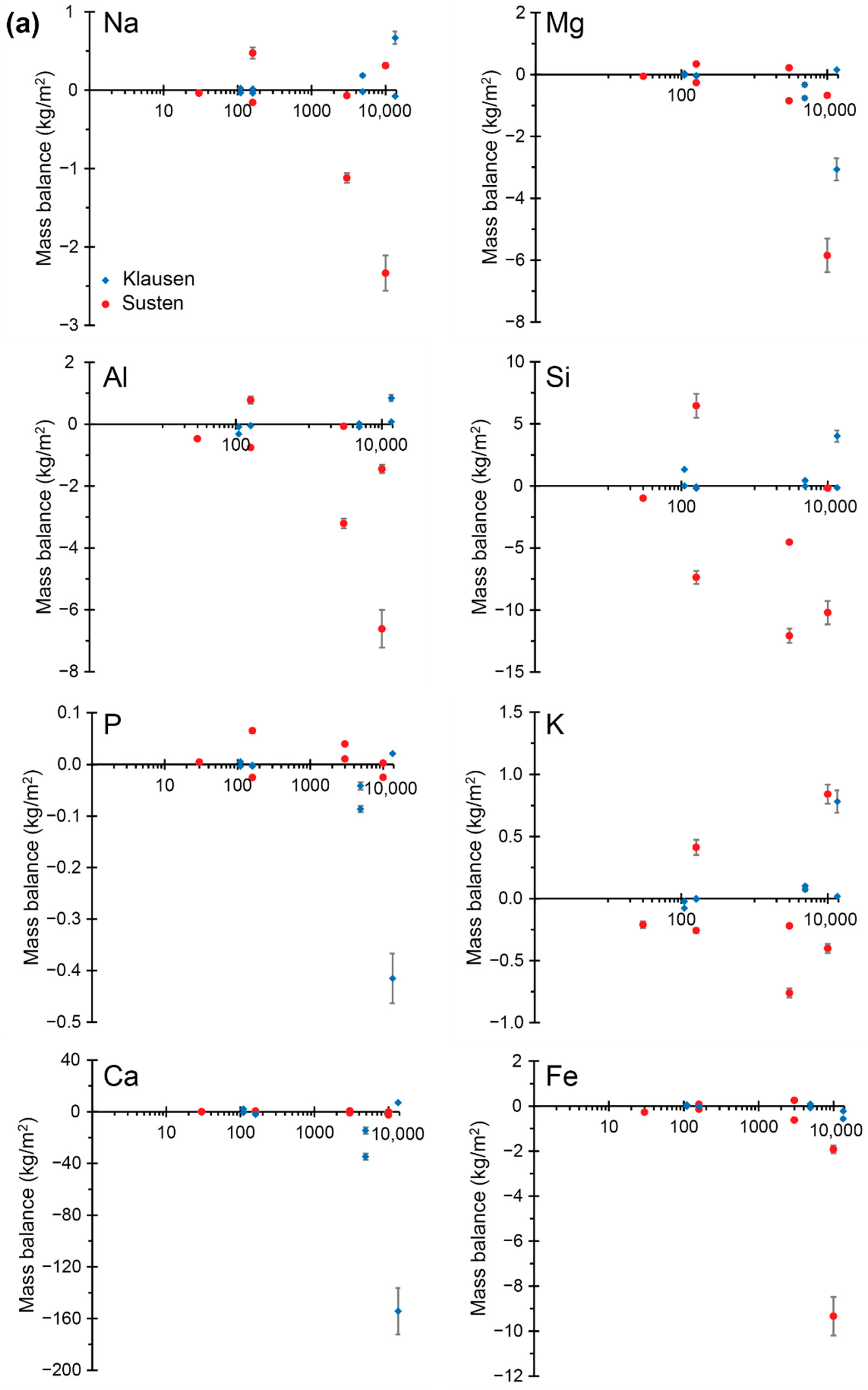
| Profile | Horizon | Depth | Mass Balance | ||||||||
|---|---|---|---|---|---|---|---|---|---|---|---|
| Na | Mg | Al | Si | P | K | Ca | Mn | Fe | |||
| cm | kg m−2 | kg m−2 | kg m−2 | kg m−2 | kg m−2 | kg m−2 | kg m−2 | kg m−2 | kg m−2 | ||
| 110 years (hyperskeletic leptosol) | |||||||||||
| K-A1 | C1 | 0–10 | −0.03 ± 0 | 0.04 ± 0 | −0.32 ± 0.02 | 1.33 ± 0.07 | 0.01 ± 0 | −0.08 ± 0 | 2.1 ± 0.11 | 0 ± 0 | 0.06 ± 0 |
| C2 | 10–20+ | 0 ± 0 | 0 ± 0 | 0 ± 0 | 0 ± 0 | 0 ± 0 | 0 ± 0 | 0 ± 0 | 0 ± 0 | 0 ± 0 | |
| K-A2 | C1 | 0–10 | 0.02 ± 0 | −0.02 ± 0 | −0.08 ± 0.01 | 0 ± 0 | 0 ± 0 | −0.02 ± 0 | −0.62 ± 0.06 | 0 ± 0 | −0.01 ± 0 |
| C2 | 10–20+ | 0 ± 0 | 0 ± 0 | 0 ± 0 | 0 ± 0 | 0 ± 0 | 0 ± 0 | 0 ± 0 | 0 ± 0 | 0 ± 0 | |
| 160 years (hyperskeletic leptosol) | |||||||||||
| K-B1 | AC | 0–15 | 0.02 ± 0 | −0.03 ± 0.01 | −0.05 ± 0.01 | −0.06 ± 0.02 | 0 ± 0 | 0 ± 0 | −1.52 ± 0.44 | 0 ± 0 | −0.02 ± 0.01 |
| C | 15–25+ | 0 ± 0 | 0 ± 0 | 0 ± 0 | 0 ± 0 | 0 ± 0 | 0 ± 0 | 0 ± 0 | 0 ± 0 | 0 ± 0 | |
| K-B2 | AC | 0–10 | −0.04 ± 0.02 | −0.05 ± 0.03 | −0.04 ± 0.03 | −0.19 ± 0.11 | 0 ± 0 | −0.01 ± 0 | −2.13 ± 1.24 | 0 ± 0 | −0.03 ± 0.02 |
| C | 10–28+ | 0 ± 0 | 0 ± 0 | 0 ± 0 | 0 ± 0 | 0 ± 0 | 0 ± 0 | 0 ± 0 | 0 ± 0 | 0 ± 0 | |
| 4900 years (calcaric skeletic cambisol) | |||||||||||
| K-C1 | A | 0–15 | 0.05 ± 0.01 | −0.19 ± 0.06 | 0.02 ± 0.01 | 0.37 ± 0.11 | −0.03 ± 0.01 | 0.05 ± 0.01 | −9.02 ± 2.69 | 0.01 ± 0 | 0.02 ± 0.01 |
| B | 15–21 | 0.02 ± 0 | −0.09 ± 0.01 | 0.01 ± 0 | 0.01 ± 0 | −0.01 ± 0 | 0.02 ± 0 | −4.07 ± 0.63 | 0 ± 0 | 0.01 ± 0 | |
| BC | 21–60 | −0.08 ± 0.01 | −0.05 ± 0 | −0.01 ± 0 | 0.05 ± 0 | 0 ± 0 | 0 ± 0 | −1.51 ± 0.12 | 0 ± 0 | 0.05 ± 0 | |
| C | 60–80+ | 0 ± 0 | 0 ± 0 | 0 ± 0 | 0 ± 0 | 0 ± 0 | 0 ± 0 | 0 ± 0 | 0 ± 0 | 0 ± 0 | |
| K-C2 | OA | 0–18 | 0.12 ± 0.01 | −0.34 ± 0.01 | −0.08 ± 0 | 0.31 ± 0.01 | −0.04 ± 0 | 0.05 ± 0 | −15.8 ± 0.4 | 0 ± 0 | −0.04 ± 0 |
| B | 18–42 | 0.08 ± 0.01 | −0.33 ± 0.05 | 0.04 ± 0.01 | 0.11 ± 0.02 | −0.04 ± 0.01 | 0.08 ± 0.01 | −15.55 ± 2.18 | 0.01 ± 0 | 0.03 ± 0 | |
| BC | 42–51 | −0.01 ± 0 | −0.09 ± 0 | −0.05 ± 0 | −0.43 ± 0 | −0.01 ± 0 | −0.02 ± 0 | −3.45 ± 0.01 | 0 ± 0 | −0.07 ± 0 | |
| C | 51–75+ | 0 ± 0 | 0 ± 0 | 0 ± 0 | 0 ± 0 | 0 ± 0 | 0 ± 0 | 0 ± 0 | 0 ± 0 | 0 ± 0 | |
| 13,500 years (calcaric skeletic cambisol) | |||||||||||
| K-D1 | A1 | 0–15 | 0.01 ± 0 | −0.07 ± 0.01 | 0 ± 0 | 0.08 ± 0.01 | −0.01 ± 0 | 0.01 ± 0 | −3.31 ± 0.53 | 0 ± 0 | −0.02 ± 0 |
| A2 | 15–28 | 0.01 ± 0 | −0.16 ± 0.02 | 0.01 ± 0 | 0.25 ± 0.03 | −0.02 ± 0 | 0.02 ± 0 | −7.88 ± 0.82 | 0 ± 0 | −0.03 ± 0 | |
| B | 28–32 | −0.01 ± 0 | −0.04 ± 0.01 | 0.01 ± 0 | 0.16 ± 0.04 | −0.01 ± 0 | 0 ± 0 | −2.03 ± 0.57 | 0 ± 0 | 0.01 ± 0 | |
| BC1 | 32–68 | −0.1 ± 0.01 | 0.43 ± 0.04 | 0.04 ± 0 | −0.63 ± 0.06 | 0.05 ± 0 | −0.01 ± 0 | 20.22 ± 1.85 | 0 ± 0 | −0.19 ± 0.02 | |
| BC2 | 68–80+ | 0 ± 0 | 0 ± 0 | 0 ± 0 | 0 ± 0 | 0 ± 0 | 0 ± 0 | 0 ± 0 | 0 ± 0 | 0 ± 0 | |
| K-D2 | OA | 0–30 | 0.66 ± 0.15 | −3.04 ± 0.68 | 0.84 ± 0.19 | 4.01 ± 0.89 | −0.41 ± 0.09 | 0.78 ± 0.17 | −153.33 ± 34.16 | −0.01 ± 0 | −0.55 ± 0.12 |
| B | 30–35 | 0.01 ± 0 | −0.02 ± 0 | 0.01 ± 0 | 0 ± 0 | 0 ± 0 | 0 ± 0 | −1 ± 0.07 | 0 ± 0 | −0.02 ± 0 | |
| BC | 35–70+ | 0 ± 0 | 0 ± 0 | 0 ± 0 | 0 ± 0 | 0 ± 0 | 0 ± 0 | 0 ± 0 | 0 ± 0 | 0 ± 0 | |
| 30 years (hyperskeletic leptosol) | |||||||||||
| S-A1 | AC | 0–10 | −0.13 ± 0.09 | −0.06 ± 0.04 | −0.47 ± 0.33 | −0.99 ± 0.7 | 0 ± 0 | −0.21 ± 0.15 | −0.04 ± 0.02 | 0 ± 0 | −0.27 ± 0.19 |
| C | 10–30+ | 0 ± 0 | 0 ± 0 | 0 ± 0 | 0 ± 0 | 0 ± 0 | 0 ± 0 | 0 ± 0 | 0 ± 0 | 0 ± 0 | |
| S-A2 | C | 0–50+ | 0 ± 0 | 0 ± 0 | 0 ± 0 | 0 ± 0 | 0 ± 0 | 0 ± 0 | 0 ± 0 | 0 ± 0 | 0 ± 0 |
| 160 years (hyperskeletic leptosol) | |||||||||||
| S-B1 | OA | 0–10 | −0.14 ± 0.03 | −0.02 ± 0 | 0.01 ± 0 | 0.19 ± 0.05 | −0.01 ± 0 | 0.09 ± 0.02 | −0.03 ± 0.01 | 0 ± 0 | −0.03 ± 0.01 |
| AC | 10–20 | −0.01 ± 0 | −0.11 ± 0.03 | −0.13 ± 0.03 | −0.87 ± 0.22 | 0 ± 0 | 0.04 ± 0.01 | −0.07 ± 0.02 | 0 ± 0 | −0.06 ± 0.01 | |
| C1 | 20–40 | 0.62 ± 0.15 | −0.13 ± 0.03 | 0.9 ± 0.22 | 7.13 ± 1.74 | −0.02 ± 0 | 0.29 ± 0.07 | 0.11 ± 0.03 | 0 ± 0 | −0.05 ± 0.01 | |
| C2 | 40–55+ | 0 ± 0 | 0 ± 0 | 0 ± 0 | 0 ± 0 | 0 ± 0 | 0 ± 0 | 0 ± 0 | 0 ± 0 | 0 ± 0 | |
| S-B2 | A | 0–10 | 0.14 ± 0.03 | 0.04 ± 0.01 | −0.44 ± 0.1 | −2.18 ± 0.49 | 0.07 ± 0.02 | −0.08 ± 0.02 | 0.65 ± 0.15 | 0.01 ± 0 | 0.03 ± 0.01 |
| C1 | 10–30 | −0.3 ± 0.05 | 0.29 ± 0.05 | −0.32 ± 0.05 | −5.2 ± 0.89 | −0.01 ± 0 | −0.17 ± 0.03 | −0.15 ± 0.03 | 0 ± 0 | 0.05 ± 0.01 | |
| C2 | 30–45+ | 0 ± 0 | 0 ± 0 | 0 ± 0 | 0 ± 0 | 0 ± 0 | 0 ± 0 | 0 ± 0 | 0 ± 0 | 0 ± 0 | |
| 3000 years (skeletic cambisol) | |||||||||||
| S-C1 | A | 0–10 | 0.14 ± 0.02 | 0.06 ± 0.01 | −0.19 ± 0.02 | −2.51 ± 0.29 | 0.01 ± 0 | −0.31 ± 0.04 | 0.64 ± 0.07 | 0.01 ± 0 | 0.19 ± 0.02 |
| B | 10–30 | −0.21 ± 0.03 | 0.15 ± 0.02 | 0.12 ± 0.02 | −2.03 ± 0.31 | 0 ± 0 | 0.08 ± 0.01 | −0.1 ± 0.02 | 0 ± 0 | 0.06 ± 0.01 | |
| BC | 30–55+ | 0 ± 0 | 0 ± 0 | 0 ± 0 | 0 ± 0 | 0 ± 0 | 0 ± 0 | 0 ± 0 | 0 ± 0 | 0 ± 0 | |
| S-C2 | A | 0–23 | −0.63 ± 0.34 | −0.49 ± 0.27 | −2.07 ± 1.13 | −8.49 ± 4.61 | 0.04 ± 0.02 | −0.59 ± 0.32 | −0.33 ± 0.18 | 0.01 ± 0 | −0.32 ± 0.17 |
| Bw | 23–40 | −0.49 ± 0.11 | −0.35 ± 0.08 | −1.13 ± 0.25 | −3.59 ± 0.79 | 0 ± 0 | −0.17 ± 0.04 | −0.51 ± 0.11 | −0.01 ± 0 | −0.3 ± 0.07 | |
| BC | 40–60+ | 0 ± 0 | 0 ± 0 | 0 ± 0 | 0 ± 0 | 0 ± 0 | 0 ± 0 | 0 ± 0 | 0 ± 0 | 0 ± 0 | |
| 10,000 years (entic podsol) | |||||||||||
| S-D1 | O | 0–20 | 0.08 ± 0.06 | −0.21 ± 0.16 | −0.31 ± 0.23 | −0.51 ± 0.37 | 0.02 ± 0.01 | −0.1 ± 0.07 | −0.12 ± 0.09 | −0.02 ± 0.01 | −0.65 ± 0.47 |
| OE | 20–36 | −0.09 ± 0.02 | −0.42 ± 0.12 | −0.78 ± 0.23 | −1.34 ± 0.39 | 0.01 ± 0 | −0.22 ± 0.06 | −0.22 ± 0.06 | −0.03 ± 0.01 | −1.21 ± 0.35 | |
| Bs | 36–63 | 0.32 ± 0.06 | −0.04 ± 0.01 | −0.36 ± 0.06 | 1.67 ± 0.3 | −0.02 ± 0 | −0.08 ± 0.01 | 0.1 ± 0.02 | 0 ± 0 | −0.07 ± 0.01 | |
| BC | 63–80+ | 0 ± 0 | 0 ± 0 | 0 ± 0 | 0 ± 0 | 0 ± 0 | 0 ± 0 | 0 ± 0 | 0 ± 0 | 0 ± 0 | |
| S-D2 | OE | 0–35 | −0.62 ± 0.23 | −2.6 ± 0.95 | −3.03 ± 1.11 | −4.58 ± 1.67 | 0.05 ± 0.02 | 0.01 ± 0 | −1.12 ± 0.41 | −0.1 ± 0.04 | −5.06 ± 1.85 |
| Bs | 35–68 | −1.72 ± 0.49 | −3.24 ± 0.91 | −3.58 ± 1 | −5.63 ± 1.58 | −0.07 ± 0.02 | 0.83 ± 0.23 | −1.43 ± 0.4 | −0.1 ± 0.03 | −4.28 ± 1.2 | |
| BC | 68–80+ | 0 ± 0 | 0 ± 0 | 0 ± 0 | 0 ± 0 | 0 ± 0 | 0 ± 0 | 0 ± 0 | 0 ± 0 | 0 ± 0 | |
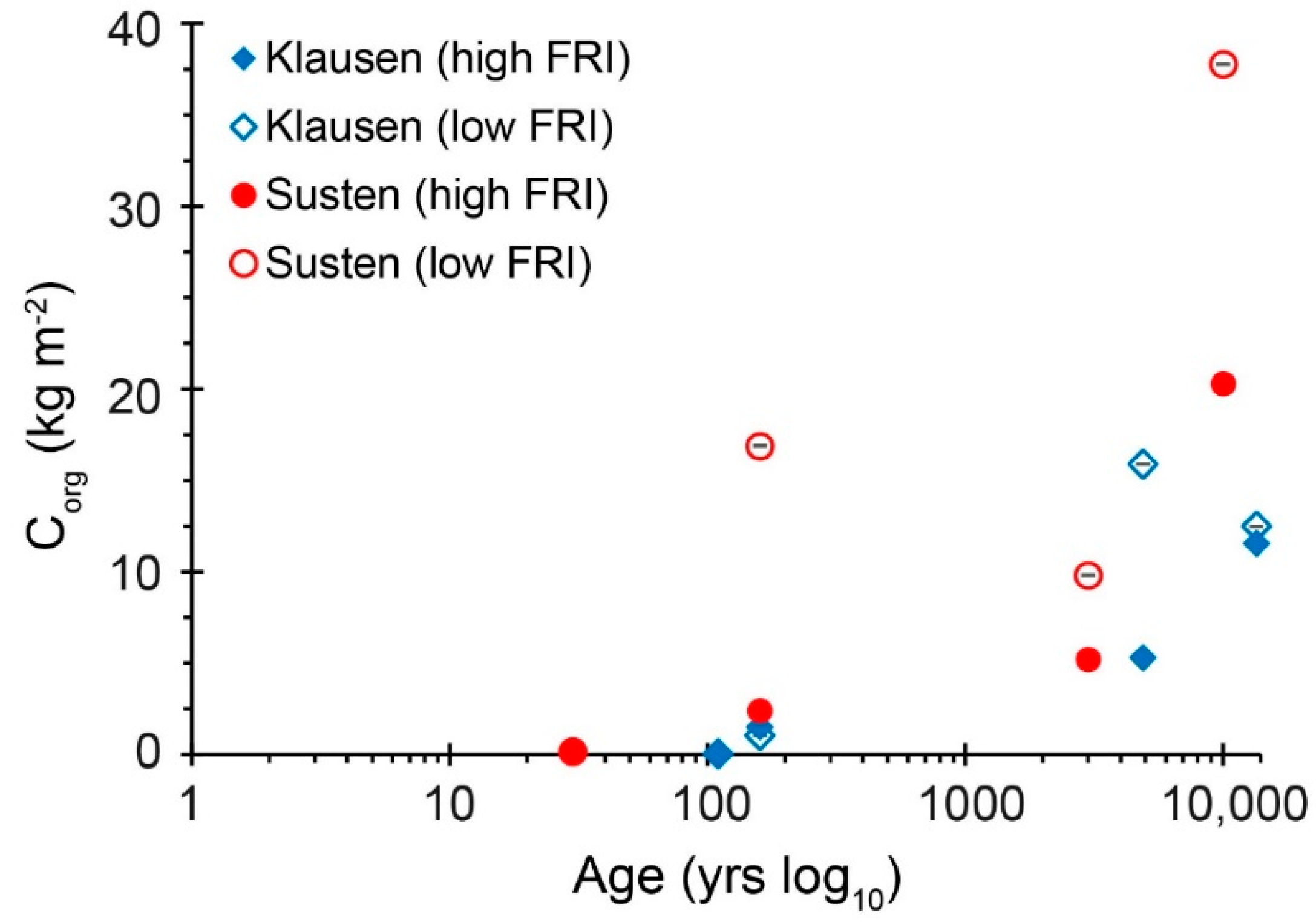
| Profile | Horizon | Depth | OM | Corg | N | C/N | Feo | Alo | Mno |
|---|---|---|---|---|---|---|---|---|---|
| cm | g kg−1 | g kg−1 | g kg−1 | mg kg−1 | mg kg−1 | mg kg−1 | |||
| Klausenpass (Griess Glacier) | |||||||||
| 110 years | |||||||||
| K-A1 | C1 | 0–10 | 17.51 | 0.96 ± 0 | 0.39 ± 0 | 2.87 ± 0 | 1494 ± 124 | 206 ± 0 | 32 ± 2 |
| C2 | 10–20+ | 19.83 | 0.29 ± 0 | 0.31 ± 0 | 1.11 ± 0 | 1390 ± 169 | 266 ± 0 | 19 ± 0 | |
| K-A2 | C1 | 0–10 | 18.95 | 0.78 ± 0 | 0.35 ± 0.02 | 2.56 ± 0.04 | 1571 ± 121 | 191 ± 0 | 53 ± 2 |
| C2 | 10–20+ | 17.91 | 0 | 0.24 * | N/A | 1545 ± 271 | 212 ± 0 | 32 ± 5 | |
| 160 years | |||||||||
| K-B1 | AC | 0–15 | 83.85 | 26.99 ± 0.18 | 2.2 ± 0.05 | 14.33 ± 0.02 | 2751 ± 158 | 293 ± 0 | 149 ± 26 |
| C | 15–25+ | 33.44 | 5.74 ± 0.06 | 0.68 ± 0.01 | 9.81 ± 0.01 | 2007 ± 91 | 215 ± 4 | 52 ± 14 | |
| K-B2 | AC | 0–10 | 89.29 | 22.07 ± 3.92 | 1.89 ± 0.33 | 13.62 ± 0.25 | 2767 ± 331 | 309 ± 48 | 157 ± 7 |
| C | 10–28+ | 32.15 | 4.84 ± 0.02 | 0.67 ± 0.02 | 8.39 ± 0.02 | 1665 ± 137 | 229 ± 0 | 41 ± 6 | |
| 4900 years | |||||||||
| K-C1 | A | 0–15 | 187.06 | 71.2 ± 0.02 | 6.71 ± 0.05 | 12.38 ± 0.01 | 6621 ± 831 | 2578 ± 183 | 671 ± 180 |
| B | 15–21 | 99.65 | 25.61 ± 0.07 | 3.35 ± 0.13 | 8.93 ± 0.04 | 7416 ± 269 | 2379 ± 211 | 758 ± 282 | |
| BC | 21–60 | 27.37 | 0.94 ± 0 | 0.68 ± 0.01 | 1.62 ± 0.02 | 2451 ± 236 | 667 ± 0 | 93 ± 0 | |
| C | 60–80+ | 22.32 | 0 | 0.42 ± 0.01 | N/A | 1739 ± 115 | 544 ± 0 | 47 ± 0 | |
| K-C2 | OA | 0–18 | 344.02 | 150.89 ± 2.98 | 11.29 ± 0.16 | 15.59 ± 0.02 | 8225 ± 377 | 2564 ± 0 | 405 ± 57 |
| B | 18–42 | 140.03 | 45.9 ± 0.17 | 5.07 ± 0.02 | 10.56 ± 0.01 | 7806 ± 1193 | 3317 ± 0 | 1040 ± 122 | |
| BC | 42–51 | 37.64 | 3.88 ± 0 | 0.92 ± 0.02 | 4.9 ± 0.02 | 2912 ± 475 | 630 ± 18 | 138 ± 11 | |
| C | 51–75+ | 27.33 | 2.12 ± 0 | 0.67 ± 0.03 | 3.68 ± 0.04 | 2065 ± 245 | 549 ± 6 | 102 ± 13 | |
| 13,500 years | |||||||||
| K-D1 | A1 | 0–15 | 424.36 | 185.86 ± 1.65 | 14.44 ± 0.19 | 15.01 ± 0.02 | 9993 ± 117 | 2059 ± 0 | 750 ± 88 |
| A2 | 15–28 | 204.90 | 78.91 ± 2.5 | 7.66 ± 0.15 | 12.03 ± 0.04 | 11,423 ± 528 | 2661 ± 132 | 724 ± 141 | |
| B | 28–32 | 57.96 | 13.82 ± 0.05 | 1.69 ± 0.02 | 9.52 ± 0.01 | 2748 ± 6 | 795 ± 0 | 262 ± 51 | |
| BC1 | 32–68 | 16.44 | 0 | 0.44 ± 0 | N/A | 465 ± 3 | 226 ± 0 | 51 ± 10 | |
| BC2 | 68–80+ | 16.36 | 0 | 0.42 ± 0.01 | N/A | 880 ± 128 | 260 ± 34 | 47 ± 5 | |
| K-D2 | O/OA | 0–30 | 244.66 | 99.66 ± 232.56 | 8.21 ± 0.09 | 14.17 ± 2.33 | 7092 ± 598 | 2102 ± 0 | 456 ± 2 |
| A | 30–35 | 22.98 | 3.06 ± 3.37 | 0.63 ± 0.03 | 5.69 ± 1.1 | 1120 ± 99 | 279 ± 58 | 46 ± 2 | |
| BC | 35–70+ | 16.75 | 0 0 | 0.35 ± 0 | N/A | 487 ± 8 | 261 ± 0 | 39 ± 1 | |
| Sustenpass (Stein Glacier) | |||||||||
| 30 years | |||||||||
| S-A1 | AC | 0–10 | 11.40 | 0.97 ± 0.19 | 0.11 ± 0 | 10.21 ± 0.2 | 1103 ± 147 | 266 ± 0 | 30 ± 0 |
| C | 10–30+ | 13.46 | 0.26 ± 0.69 | N/A | N/A | 1436 ± 230 | 575 ± 0 | 35 ± 0 | |
| S-A2 | C | 0–50+ | 8.39 | 0.39 ± 3.49 | N/A | N/A | 1460 ± 243 | 413 ± 0 | 27 ± 1 |
| 160 years | |||||||||
| S-B1 | OA | 0–10 | 44.35 | 2.07 ± 2.95 | 0.3 ± 0.01 | 8.2 ± 1.42 | 1184 ± 107 | 433 ± 0 | 33 ± 0 |
| AC | 10–20 | 17.48 | 1.4 * | 0.19 * | 8.73 * | 1160 ± 58 | 308 ± 0 | 26 ± 0 | |
| C1 | 20–40 | 13.04 | 1.21 * | 0.11 * | 12.43 * | 1342 ± 15 | 290 ± 0 | 34 ± 0 | |
| C2 | 40–55+ | 10.95 | 7.37 ± 19.26 | 1.24 ± 0.02 | 6.93 ± 2.61 | 1033 ± 90 | 256 ± 0 | 21 ± 1 | |
| S-B2 | A | 0–10 | 384.24 | 105.65 ± 12.63 | 12.48 ± 0.01 | 9.88 ± 0.12 | 1228 ± 140 | 653 ± 0 | 97 ± 4 |
| C1 | 10–30 | 17.53 | 1.96 * | 0.29 * | 7.9 * | 1111 ± 138 | 337 ± 60 | 29 ± 3 | |
| C2 | 30–45+ | 14.61 | 1.03 * | 0.21 * | 5.72 * | 885 ± 112 | 286 ± 0 | 29 ± 1 | |
| 3000 years | |||||||||
| S-C1 | A | 0–10 | 34.09 | N/A | N/A | N/A | 2829 ± 283 | 1009 ± 26 | 64 ± 2 |
| B | 10–30 | 27.96 | 2.53 ± 0.71 | 0.57 ± 0 | 5.14 ± 0.28 | 2104 ± 217 | 549 ± 0 | 47 ± 0 | |
| BC | 30–55+ | 19.46 | 1.66 ± 5.55 | 0.21 ± 0.01 | 9.3 ± 3.35 | 2451 ± 414 | 283 ± 83 | 42 ± 2 | |
| S-C2 | A | 0–23 | 225.12 | 27.96 ± 4.43 | 8.31 ± 0.08 | 3.93 ± 0.16 | 3238 ± 469 | 1274 ± 0 | 297 ± 49 |
| Bw | 23–40 | 130.40 | 10.6 ± 7.65 | 4 ± 0.03 | 3.09 ± 0.72 | 1862 ± 383 | 466 ± 100 | 108 ± 44 | |
| BC | 40–60+ | 24.39 | 1.34 ± 0.39 | 0.53 ± 0.01 | 2.95 ± 0.29 | 1565 ± 264 | 435 ± 0 | 98 ± 20 | |
| 10,000 years | |||||||||
| S-D1 | O | 0–20 | 439.81 | 54.34 ± 142.12 | 13.71 ± 0.39 | 4.62 ± 2.62 | 6726 ± 232 | 3797 ± 110 | 3 ± 0 |
| OE | 20–36 | 287.40 | 70.42 ± 65.93 | 9.26 ± 0.1 | 8.88 ± 0.94 | 8226 ± 438 | 4023 ± 0 | 1 ± 0 | |
| Bs | 36–63 | 52.24 | 6.51 * | 0.71 * | 10.78 * | 9394 ± 1206 | 3874 ± 0 | 183 ± 18 | |
| BC | 63–80+ | 61.37 | 10.3 * | 1.04 * | 11.6 * | 9887 ± 1655 | 3474 ± 362 | 186 ± 4 | |
| S-D2 | OE | 0–35 | 379.81 | 159.29 ± 25.03 | 11.83 ± 0.01 | 15.71 ± 0.16 | 7347 ± 469 | 4773 ± 0 | 4 ± 2 |
| Bs | 35–68 | 99.77 | 21.03 * | 2.09 * | 11.75 * | 11,650 ± 860 | 5502 ± 0 | 59 ± 2 | |
| BC | 68–80+ | 159.53 | 11.63 * | 2.83 * | 4.79 * | 13,020 ± 230 | 9754 ± 0 | 146 ± 5 | |
| Profile | Horizon | Thickness | Bulk Density | Fine Earth | Skeleton | 10Be | 10Be | Erosion Rates | |||
|---|---|---|---|---|---|---|---|---|---|---|---|
| (conc.) | (per Horizon) | Equation (10) 1 | Equation (10) 2 | Equation (10) 3 | Equation (13) | ||||||
| (cm) | (g cm−3) | (g cm−2) | (wt. %) | (at g−1 108) | (at cm−2 108) | (t ha−1 year−1) | (t ha−1 year−1) | (t ha−1 year−1) | (t ha−1 year−1) | ||
| Klausenpass 4900 years | |||||||||||
| K-C1 | A | 15 | 0.50 | 7.45 | 11.31 | 13.32 ± 0.63 | 87.94 ± 4.15 | 0.26 ± 0.15 | −0.30 ± 0.17 | 0.17 ± 0.10 | −80 ± 0.10 |
| B | 6 | 0.74 | 4.44 | 64.47 | 10.84 ± 0.48 | 17.11 ± 0.76 | |||||
| BC | 39 | 1.53 | 59.62 | 77.93 | 1.12 ± 0.07 | 14.76 ± 0.88 | |||||
| C | 20 | 1.48 | 29.53 | 85.30 | 0.63 ± 0.03 | 2.75 ± 0.12 | |||||
| Klausenpass 13,500 | |||||||||||
| K-D1 | A1 | 15 | 0.33 | 4.94 | 6.88 | 15.29 ± 0.53 | 70.33 ± 2.44 | 0.01 ± 0.00 | −0.38 ± 0.08 | −0.05 ± 0.010 | −0.15 ± 0.02 |
| A2 | 13 | 0.48 | 6.19 | 40.85 | 17.39 ± 0.91 | 63.73 ± 3.34 | |||||
| B | 4 | 0.81 | 3.22 | 73.46 | 5.31 ± 0.15 | 4.54 ± 0.13 | |||||
| BC1 | 36 | 1.63 | 58.63 | 75.00 | 1.26 ± 0.04 | 18.5 ± 0.59 | |||||
| BC2 | 12 | 1.65 | 19.81 | 75.00 | 1.46 ± 0.04 | 7.24 ± 0.21 | |||||
| Sustenpass 3000 years | |||||||||||
| S-C1 | A | 10 | 1.31 | 13.06 | 50.41 | 1.04 ± 0.03 | 6.76 ± 0.23 | −2.64 ± 0.38 | −14.11 ± 2.03 | −4.58 ± 0.66 | −11.26 ± 0.20 |
| B | 20 | 1.51 | 30.28 | 68.90 | 0.3 ± 0.01 | 2.85 ± 0.12 | |||||
| BC | 25 | 1.90 | 47.57 | 63.43 | 0.17 ± 0.01 | 2.89 ± 0.19 | |||||
| Sustenpass 10,000 years | |||||||||||
| S-D1 | O | 20 | 0.73 | 14.62 | 74.37 | 3.55 ± 0.1 | 13.3 ± 0.39 | −0.60 ± 0.20 | −5.27 ± 1.75 | −1.39 ± 0.46 | −1.95 ± 0.27 |
| OE | 16 | 0.71 | 11.36 | 47.94 | 3.31 ± 0.1 | 19.58 ± 0.57 | |||||
| Bs | 32 | 1.29 | 41.16 | 54.76 | 1.31 ± 0.05 | 24.31 ± 0.88 | |||||
| BC | 12 | 1.35 | 16.22 | 41.75 | 1.55 ± 0.06 | 14.68 ± 0.54 | |||||
| Moraine | Age | Soil Formation | Soil Erosion 1 | Soil Weathering | Soil Production | ||
|---|---|---|---|---|---|---|---|
| Equation (15) | (239+240Pu) | (10Be) | (Figure 5b) | Equation (1) 2 | |||
| (years) | mm year−1 | t ha−1 year−1 | t ha−1 year−1 | t ha−1 year−1 | t ha−1 year−1 | t ha−1 year−1 | |
| Klausenpass (Griess Glacier) | |||||||
| K-A | 110 | 0.00 | 0.00 | −10.23 | N/A | 0.11 | 10.34 |
| K-B | 160 | 0.78 | 6.24 | −4.15 | N/A | −0.13 | 10.52 |
| K-C | 4900 | 0.12 | 1.92 | −1.04 | 0.05 | −0.05 | 2.02 |
| K-D | 13,500 | >0.06 * | 1.08 | −0.32 | −0.14 | −0.05 | 1.27 * |
| Sustenpass (Stein Glacier) | |||||||
| S-A | 30 | 1.65 | 28.05 | N/A | N/A | −0.69 | 34.15 ** |
| S-B | 160 | 0.94 | 17.86 | −5.41 | N/A | 0.00 | 23.27 |
| S-C | 3000 | >0.19 * | >3.42 * | −2.65 | −7.11 | −0.04 | 10.57 * |
| S-D | 10,000 | >0.08 * | >1.04 * | −1.92 | −2.42 | −0.02 | 3.48 * |
Publisher’s Note: MDPI stays neutral with regard to jurisdictional claims in published maps and institutional affiliations. |
© 2022 by the authors. Licensee MDPI, Basel, Switzerland. This article is an open access article distributed under the terms and conditions of the Creative Commons Attribution (CC BY) license (https://creativecommons.org/licenses/by/4.0/).
Share and Cite
Musso, A.; Tikhomirov, D.; Plötze, M.L.; Greinwald, K.; Hartmann, A.; Geitner, C.; Maier, F.; Petibon, F.; Egli, M. Soil Formation and Mass Redistribution during the Holocene Using Meteoric 10Be, Soil Chemistry and Mineralogy. Geosciences 2022, 12, 99. https://doi.org/10.3390/geosciences12020099
Musso A, Tikhomirov D, Plötze ML, Greinwald K, Hartmann A, Geitner C, Maier F, Petibon F, Egli M. Soil Formation and Mass Redistribution during the Holocene Using Meteoric 10Be, Soil Chemistry and Mineralogy. Geosciences. 2022; 12(2):99. https://doi.org/10.3390/geosciences12020099
Chicago/Turabian StyleMusso, Alessandra, Dmitry Tikhomirov, Michael L. Plötze, Konrad Greinwald, Anne Hartmann, Clemens Geitner, Fabian Maier, Fanny Petibon, and Markus Egli. 2022. "Soil Formation and Mass Redistribution during the Holocene Using Meteoric 10Be, Soil Chemistry and Mineralogy" Geosciences 12, no. 2: 99. https://doi.org/10.3390/geosciences12020099